HAL Id: hal-00468567
https://hal.archives-ouvertes.fr/hal-00468567
Submitted on 31 Mar 2010
HAL is a multi-disciplinary open access
archive for the deposit and dissemination of
sci-entific research documents, whether they are
pub-lished or not. The documents may come from
teaching and research institutions in France or
abroad, or from public or private research centers.
L’archive ouverte pluridisciplinaire HAL, est
destinée au dépôt et à la diffusion de documents
scientifiques de niveau recherche, publiés ou non,
émanant des établissements d’enseignement et de
recherche français ou étrangers, des laboratoires
publics ou privés.
E. Masse, C. Curt, M. Le Goc
To cite this version:
E. Masse, C. Curt, M. Le Goc. Forecasting embankment dam behaviour with artificial intelligence.
12th International Conference of International Association for Computer Methods and Advances in
Geomechanics (IACMAG), Oct 2008, Goa, India. 8 p. �hal-00468567�
Forecasting embankment dam behaviour with artificial intelligence
Emilie Masse
1,2, Corinne Curt
11
Cemagref Aix-en-Provence – Unité OHAX – 3275 Route de Cézanne – CS 40061 – 13182 Aix en Provence Cedex 5 – France
Marc Le Goc
2 2LSIS Laboratoire des Sciences de l’Information et des Systèmes – UMR CNRS 6168 – Université Paul Cézanne Aix-Marseille III – Avenue Escadrille Normandie Niemen – 13397 Marseille Cedex 20 – France
Keywords: expert knowledge, multi model approach, dam behaviour
ABSTRACT: Forecasting dam behaviour is of paramount importance to avoid collapses. It consists of detecting and controlling deterioration mechanisms. This paper sets out to propose a multi model methodology to model complex dynamic systems, such as dams. It defines three models based on expert knowledge: a structural model, a functional model and a behavioural model. They are developed from the stories of the ageing of the processes that is to say from scenarios described in terms of events. These scenarios are interpreted by expert knowledge. One of the main ideas is to use the level of abstraction of the experts to facilitate the problem solving reasoning. A conceptual model which is created from CommonKADS methodology allows us to divide consistently the knowledge base into the three models. We illustrate this methodology by monitoring the dam behaviour during its life. Currently, the three models are developed from the scenario of the ageing of a French dam. They are validated by experts who gave their accordance with the developed approach. These models show that it is possible to formalize models implicitly used by experts.
1 Introduction
Forecasting dam behaviour is fundamental to prevent accidents and to determine corrective measures. Forecasting means detecting and controlling deterioration mechanisms which can cause the collapse of a dam if no measure is taken, such as maintenance or emergency release. These deteriorations are caused by many more or less dependent dynamic processes, such as clogging, internal erosion, sliding, having various and often multiple sources. Curt et al. (2006) have conducted a research showing that it is possible to assess the performance of a dam at a given time from formalized and aggregated information of various data natures, such as, visual observations, data from auscultation, data from mechanical models and conception or implementation data. However, the dynamic aspect of these processes poses the problem of the acquisition and the representation of the underlying temporal knowledge because this temporality is often mixed with other types of knowledge, such as structure, variables (Basseville and Cordier, 1996). Answering this issue leads us to combine CommonKads methodology (Schreiber et al., 2000) with a multi model diagnosis approach (Chittaro et al., 1993). This paper aims at proposing a multi model methodology to design a support system for prediction and control of dam behaviour. Section 2 presents basis of our modelling methodology and explains the importance of maintaining the coherence of the models. Section 3 shows an illustration concerning a dam that suffered from internal erosion and presents what the perspectives are to improve the developed modelling approach. Finally, section 4 states our conclusions and gives future perspectives on our work.
2 Developed Approach
2.1 Presentation
This paper presents a part of a method used to represent a dynamic process using the same level of abstraction that an expert uses when diagnosing. We propose to combine a multi model approach with the CommonKADS conceptual method to offset drawbacks of each method. The multi model approach proposed by Chittaro et al. (1993) is concerned with a computational problem linked with the number of components declared in the structure (Zouaoui, 1998). This problem is directly linked with the abstraction level which is defined by designers because the structure is the one of the design model. CommonKADS is a problem solving method which uses expert knowledge and formalises the expert reasoning in a conceptual model. CommonKADS leads us to use knowledge bases of expert knowledge in our approach to catch the level of abstraction used by experts, and then, to use it in the models. This level of abstraction corresponds to a level of aggregation that minimizes the set of
components. So, this minimizes the computational problem because the abstraction level of the models is not the one of the designers but the one used by experts to have efficient diagnoses of the process. This method aims at representing the implicit models of the Experts and is directed with the timed observations the Experts use to diagnose.
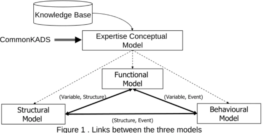
This approach (figure 1) is divided into two parts (Le Goc and Masse, 2007). First, we propose to use a CommonKads conceptual model to analyze and represent interpretative knowledge contained in a knowledge base (Schreiber et al., 2000). Such a conceptual model is an instantiation of a CommonKads template of a cognitive task. Second, this conceptual model is used to interpret the knowledge base and to distinguish fundamental knowledge. This knowledge is represented by three models adapted from a multi model approach (Chittaro et al., 1993) to the Zanni’s conceptual framework (Zanni et al., 2005): a structural model, a functional model and a behavioural model. The structural model describes relations among components of the system as a dam. It will be defined as an organised set of physical relations between components or aggregates. The functional model describes relations (i.e. mathematical functions) that link various variables of the system; each variable represents an element of the structural model (i.e. a component). Each function allows a value affectation of output variable according to input variables. A functional model may be defined as an organised set of logical relations defining the values of variables. The behavioural model describes the states of the system and the discrete events which represent state transitions. A discrete event is defined as the affectation of a value to a variable. A behavioural model is then a set of sequential relations between states. These sequential relations can be conditioned with predicates concerning the occurrence of discrete events. A discrete event is defined according to the spatial discretization principle of the Stochastic Approach (Le Goc et al, 2005) as a couple (x, δ)
where x is a symbol denoting a variable and δ is a value for x so that a discrete event occurrence is triplet (x, δ, tk) meaning: x(tk)=δ where tk means a point in time.
The knowledge base is interpreted by the conceptual model with the aim of separating knowledge to represent the system with the three models. The knowledge base may be seen as the story of the ageing of the processes. Scenarios described in terms of events allow the designing of the behavioural model. Defining a state as a set of values linked with variables of the system, the functional model may be deduced.
Knowledge Base Expertise Conceptual Model Functional Model Behavioural Model Structural
Model (Structure, Event)
(Variable, Event) (Variable, Structure)
CommonKADS
Figure 1 . Links between the three models
2.2 Coherence of the models
The modelling process is based on maintaining coherence among the three models: a piece of knowledge must be fitted into one of the three models and must not introduce incoherence into the other models. Otherwise, repeating the process until an incoherence is unsolved, leads to modelling being stopped. The other condition for stopping modelling is an appropriate completeness level to solve the problem with coherence models. The functional, structural and behavioural models are linked with the notion of variable (See figure 1) because (i) a variable used by a function of the functional model represents a structural model element and a discrete event is defined as a value affectation to a variable. There exist three relations. The first one links each output of a component “ci” with at least one variable “xi”. The second relation links the output of a function fi(x1(t),x2(t), ...,xm(t)) with at least one variable “xi”. The third one links each state transition with at least one variable xi through a class definition Ci = {(xi,δi)}. Thus, coherence is mainly controlled by the functional model which is the “pivot” between the behavioural model and the structural model.
3 Application
Cemagref centre of Aix-en-Provence (France). The knowledge base relates the story of the Cublize dam and its diagnosis. It is a formalized expertise composed of: dam section (See Figure 2), text and curves giving the diagnosis and describing the evolution concerning the history of the ageing of the dam for 10 years that is to say the deterioration scenario of Cublize dam.
Crest : 442
Upstream berm : level 433 Downstream berm : level 433 Normal water level elevation : 439
Interface foundation fill Anchorage trench
Vertical drain : level 437
sensor
sensor sensor
Crest : 442
Upstream berm : level 433 Downstream berm : level 433 Normal water level elevation : 439
Interface foundation fill Anchorage trench
Vertical drain : level 437
sensor
sensor sensor
Figure 2 . Section of Cublize dam
3.1 The Cublize dam description
This methodology was applied to a French homogeneous earth dam called the Cublize dam. It comprises a vertical drain whose top is 2m lower than the normal water level and a horizontal drain at the foundation interface over the dam halfway downstream. Investigations concluded that a mechanism of internal erosion was operative. Firstly, clogging caused the gradual saturation of the upstream fill. Secondly the infiltration water overtopped the drain which consequently saturated the downstream fill.
3.2 Results
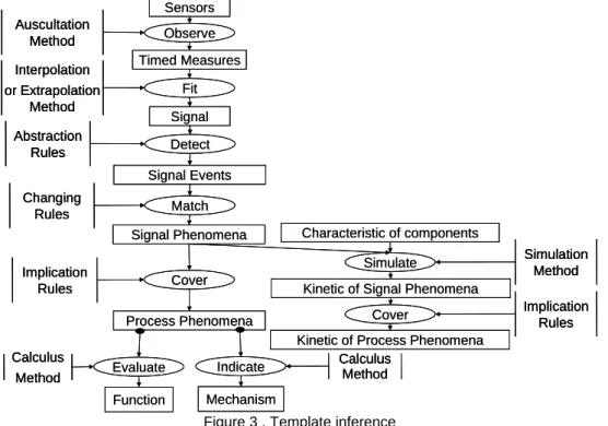
The first step of the knowledge analysis aims to prepare knowledge to be fitted into the three defined models. CommonKADS leads to design a conceptual model used to interpret knowledge. It is nearly the same as one defined in a previous project concerning blast furnaces used by Sachem system (Le Goc, 2004). Figure 3 is the inference template developed from knowledge of dam experts that is to say the way followed by experts to link a sensor with process phenomena. Thereby, this template explains how a sensor measures values which capture signal phenomena. After, experts interpret signal phenomena as process phenomena. For example, signal from a pressure sensor gives information on the phenomenon “water infiltration in the downstream fill”.
Sensors Observe Timed Measures Signal Signal Phenomena Process Phenomena Function Fit Match Cover Evaluate Interpolation or Extrapolation Method Calculus Method Changing Rules Implication Rules Mechanism Indicate Calculus Method Signal Events Detect Abstraction Rules Auscultation Method Characteristic of components Simulate
Kinetic of Process Phenomena Kinetic of Signal Phenomena
Simulation Method Cover Implication Rules Sensors Observe Timed Measures Signal Signal Phenomena Process Phenomena Function Fit Match Cover Evaluate Interpolation or Extrapolation Method Interpolation or Extrapolation Method Calculus Method Calculus Method Changing Rules Changing Rules Implication Rules Implication Rules Mechanism Indicate Calculus Method Calculus Method Signal Events Detect Abstraction Rules Abstraction Rules Auscultation Method Auscultation Method Characteristic of components Simulate
Kinetic of Process Phenomena Kinetic of Signal Phenomena
Simulation Method Simulation Method Cover Implication Rules Implication Rules
This analysis allows us to design four kinds of list of: components, variables linked with components, sets of values of each variable and event occurrences.
3.2.1 Structural model
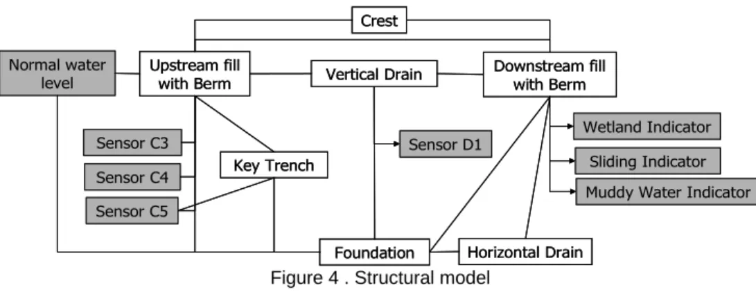
The Cublize dam section (See Figure 2) and the listing of components lead to the structural model of Figure 4. The structural model is a graph of binary relations which represent connections among structures. In this example, there are eight sensors coloured in grey shown in Figure 4 and seven components. Sensors C3, C4 and C5 are pressure sensors and sensor D1 is a flow sensor whereas wetland indicator, sliding indicator and muddy water indicator are some visual observations formalised by Curt et al. (2006).
Downstream fill with Berm Vertical Drain Upstream fill with Berm Crest Foundation Sensor C3 Sensor C4 Sensor C5 Sensor D1 Horizontal Drain Key Trench Normal water level Wetland Indicator Sliding Indicator Muddy Water Indicator Downstream fill with Berm Vertical Drain Upstream fill with Berm Crest Foundation Sensor C3 Sensor C4 Sensor C5 Sensor D1 Horizontal Drain Key Trench Normal water level Wetland Indicator Sliding Indicator Muddy Water Indicator
Figure 4 . Structural model
A variable noted “xi” is assigned to each element of the structural model (See Table 1). The value of the variable “xi” is noted “δ”.
Table 2: Value tables
PhSg20, 21 Normal water level
x8
PhSg17 Sliding indicator on the downstream fill
x7
PhSg18, 19 Muddy Water indicator on the downstream fill
x6
PhSg15, 16, 19 Wetland indicator on the downstream fill
x5
PhSg6, 12, 13, 14 Flow sensor D1 in the vertical drain
x4
PhSg5, 8, 10 Pressure sensor C5 in the upstream fill
x3
PhSg4, 7, 9 Pressure sensor C4 in the upstream fill
x2
PhSg1, 2, 3, 11 Pressure sensor C3 in the upstream fill
x1
PhSg observed by sensors Sensors linked with Components
Variables
3.2.2 Behavioural model
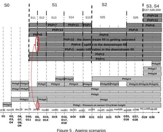
With the conceptual analysis of the knowledge base, it is possible to identify and distinguish between signal phenomena (PhSg) and process phenomena (PhPr). A signal phenomenon is an observable signal at a given time provided by a sensor whereas a process phenomenon is a unobservable signal. Each signal phenomenon is interpreted by experts as a process phenomenon. Thereby, PhSg1 meaning: “Pressure on sensor C3 ≥ Drain height” is interpreted as “water infiltration in the downstream fill” (PhPr3), as “uplifts in the downstream fill” (PhPr4) and as “the downstream fill is getting saturated” (PhPr10) (See red ovals and arrow on Figure5). A process phenomenon occurrence is deduced to a signal evolution (signal phenomenon, PhSg) provided by specific sensors represented by a variable. Thereby, a process phenomenon is linked with at least one variable through signal phenomenon. It is important to strictly list discrete event occurrences of the form ok ≡ (tk, x, i) concerning the start of signal phenomena which denotes state transitions. Given that last example, discrete event occurrences can be written as ok ≡ (July 80, x1, ≥430) linked with the start of PhSg1. The scenario of ageing of the dam can be represented from the list of event occurrences as shown in Figure 5.
O2, O3, O4 O6, O7, O8, O9 O10, O11 O5, O12 O15 O13, O14 O24 O16, O17, O18
O19 O20 O21 O22 O23 O25, O26
O27,
O28 O29 O30 O1
dec78 avr79 juil80 nov80 oct81 nov81 dec81 oct82 oct84 nov85 dec85mars86sept88oct88 Mi oct88dec88 nov78
oct78
PhPr1 PhPr2
PhPr3 : water infiltration in the downstream fill PhPr4 : uplifts in the downstream fill
PhPr5
PhPr10 : the downstream fill is getting saturated PhPr7 PhPr7 PhPr8 PhPr9 PhPr6 PhPr11 PhPr12 PhPr14 PhPr15
PhSg1 : Pressure on sensor C3 ≥≥≥≥Drain height PhSg11 PhSg21 PhSg3 PhSg12 PhSg7 PhSg9 PhSg8 PhSg10 PhSg5 PhSg2 PhSg6 PhSg13 PhSg20 PhSg21 PhSg20 PhSg21 PhSg12 PhSg14 PhSg20 PhSg18 PhSg17 PhSg19 (PhSg16,PhSg15) PhSg4 S14 S12 S13 S11 S13 S25 S26 S37,S48,S59 S1 S2 S3, S4 S0
Figure 5 . Ageing scenarios
Evolution analysis of process phenomenon leads to the behavioural model shown in Figure 6. Indeed, starting or ending process phenomena enabled the different states to be bound. States are defined as a value modification of one or more variables. Thus, ten different states may be found. Moreover, some of them can be clustered in more general states, such as S1, S2, S3 or S4.
Naturally, Figure 6 is not the complete behavioural model but only the part on the deterioration story provided by the PHD chapter by Peyras (2003). This part of the behavioural model represents an abnormal behaviour of the dam. The normal behaviour is implicit and is not described in the PHD chapter.
S11 ∆T11 S13 S0 Deterioration detected by PhSg4, PhSg5 Action detected by ¬PhSg12,PhSg13 S59 Repairing S12 ∆T12 S14∆T13 S25 ∆T14 S48 ∆T4 S47 ∆T5 S36 ∆T3
Figure 6 . Behavioural model
It is important to distinguish two kinds of transition. Temporal transitions are autonomous transitions which represent the time spent to pass from S11 to S12. This time represents deterioration that is to say the ageing of dam. The other transitions are not autonomous because they require the deterioration of a component or a repairing action detected by a PhSg on a sensor to move to another state. For instance, S11 occurs after abnormal signals are identified on PhSg4 and PhSg5.
3.2.3 Functional model
The state transitions are defined as a value modification of at least one variable from normal value to abnormal value or conversely a change from abnormal to normal. Moreover, each state can be described as a set of variables linked with the variable values. Defining states and transitions, it is now possible to deduce a functional
model from the behavioural model shown in Figure 6. Indeed, when the process is in a particular state, the linked process phenomenon occurrences cause the evolution of the values of the variables. Some of these evolutions are some highlights. They are concerned with a discrete event that causes a new state transition. Consequently, in a first analysis, a function can be linked with each state of the behavioural model. This relation associates the values of the variables with the discrete events of the state transitions. They are linked with the considered state. This principle leads to the following functional model shown in Figure 7.
F2
F1
F3
F4
x1
x2
x4
x3
x5
x6
x7
F5
F2
F1
F3
F4
x1
x2
x4
x3
x5
x6
x7
F5
Figure 7 . Functional model
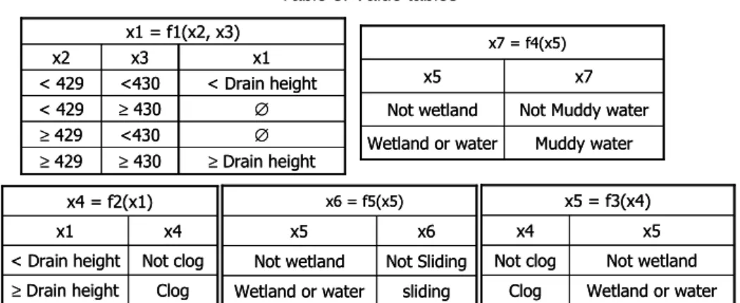
Thus, the value tables (Table 2) linked with the functional model (Figure 6) can be filled in by associating input variable values to output variable values. A function has only one output variable but may have one or more input variables.
Table 3: Value tables
Wetland or water Clog Not wetland Not clog x5 x4 x5 = f3(x4) Wetland or water Clog Not wetland Not clog x5 x4 x5 = f3(x4) ≥Drain height ≥430 ≥429 ∅ <430 ≥429 ∅ ≥430 < 429 < Drain height <430 < 429 x1 x3 x2 x1 = f1(x2, x3) ≥Drain height ≥430 ≥429 ∅ <430 ≥429 ∅ ≥430 < 429 < Drain height <430 < 429 x1 x3 x2 x1 = f1(x2, x3) Muddy water Wetland or water
Not Muddy water Not wetland x7 x5 x7 = f4(x5) Muddy water Wetland or water
Not Muddy water Not wetland x7 x5 x7 = f4(x5) Clog ≥Drain height Not clog < Drain height x4 x1 x4 = f2(x1) Clog ≥Drain height Not clog < Drain height x4 x1 x4 = f2(x1) sliding Wetland or water Not Sliding Not wetland x6 x5 x6 = f5(x5) sliding Wetland or water Not Sliding Not wetland x6 x5 x6 = f5(x5)
The first table of table 3, concerning the function f1, specifies the value of “x1” given the values of x2 and x3. The structural model (figure 4), the behavioural model (figure 6) and the functional model (figures 7) constitute the “a priori” knowledge about the Cublize dam for an internal erosion mechanism. These models were validated by Experts. Moreover, these models are an operational aid finalizing knowledge acquisition and the modelling step with experts. They produces then a set of models of the process called M(S)=<SM(S),FM(S),BM(S)> that is coherent with the scenario S={oi(tk)≡(δi,k)} when formulated as a series of occurrences oi(tk) of discrete event classes Ci = {(xi,δi)}. This scenario model will lead us to formulate some limitation of the process and its constraints. Constraints mean the goal of the process, the normal process operations and the abnormal process operations.
The previous results are only linked with the ageing process of Cublize dam which suffered of suffusion. It is important to ensure maintaining the coherence of the three models and complete models with other scenarios. We focus on continuing our work to develop our modelling approach with the tetrahedron of states (i.e. T.O.S) (Rosenberg and Karnopp, 1983) shown in Figure 8.
T.O.S. may allow us to classified on the basis of the role they play in physical phenomena interpreted as flow structure (Chittaro et al., 1993) that is to say to identify the kind of variables of the system, such as effort, displacement, flow and momentum.
It is possible to identify two different kinds of generalised variables. First, generalized substance (gs) represents the abstract entities which flow through a system. The gs concept can be further divides into two subtypes: generalised displacement (q(t)) and generalised impulse (p(t)). Second, generalized current (gc) represents the amount of a generalized substance which flows through a unitary surface in a time unit (gc = d(gs)/dt). therefore, according to the kind of gs which is flowing, two subtypes may be identify: generalised flow (f(t)) intended as flow of displacement (dq(t)/ dt) and generalized effort (e(t)) intended as flow of impulse (dp(t)/dt). The product of e * f represents the amount of energy which flows through a unitary surface in a time unit that is to say the power. After having classified physical variables, T.O.S. may be used in order to identify a set of five abstract relationships among generalized variables which are called generalized equations and are common to a large
class of physical theories. Two of them are structural equations: f(t) = dq(t)/dt and e = dp(t)/dt. The remaining three equations are constitutive equations which describe:
o The first equation is an explicit relationship between generalized effort “e” and generalized deplacement “q” involving the accumulator parameter C = dq(t)/de(t) which represent a generalized capacity F1(q(t), C, e(t)) : q(t)=C*e(t)
o The second equation is an explicit relationship between generalized effort “e” and generalized flow “f” involving the conductor parameter R = de(t)/df(t) which represent a generalized resistor F2(e(t), R, f(t)) : e(t)=R*f(t)
o The third equation is an explicit relationship between generalized impulse “p” and generalized flow “f” involving the accumulator parameter L = dp(t)/df(t) which represents a generalized inductance F3(p(t), L, f(t)) : p(t)=L*f(t). q(t) e(t) f(t) p(t) q(t) = C*e(e) p(t) = L*f(t) Displacement [m3] Momentum [N.m-2.s] e(t) = R*f(t) Flow [m3.s-1] Effort [N.m-2] f(t)=dq(t)/dt e(t)=dp(t)/dt Type 1 : Accumulator [m2. kg-1.s2] Type 2 : Conductor [kg.m-2.s-1] Type 1 : Accumulator [kg.m-1.s-1] Type 4 : Differential Type 4 : Differential
Figure 8 . The tetrahedron of states (i.e. T.O.S.)
Using the tetrahedron of states (Rosenberg and Karnopp, 1983) provides a ”physical” dimension to the variables “xi” of a process P(t) such as a dam so that an interpretation of the relations linking the variables can be deduced. This interpretation and the limitation of the process and its constraints lead to the M(P(t)) model that is called ”the generic model” of the process because it is independent of the concrete instrumentation.
Moreover, T.O.S. (Figure 8) allows a person who does not know the area of dams to make an analogy in a field in which it is more comfortable and to understand how the system works. An analogy may also offer a neutral reflection framework which fines down the data exchange between experts and non experts. Indeed, the expert must fine down his expert knowledge expression and adapt his knowledge to another domain to be understandable; it cannot be done by a non expert person.
4 Conclusions and perspectives
This paper presents the basis of a multi model methodology. These basis are a knowledge interpretation step using a CommonKADS conceptual model to interpret the knowledge base in order to fit knowledge into the three models: (1) a structural model describing relations among the components; (2) a functional model describing relations which determine affectation of a possible value to a variable; (3) a behavioural model describing the states of the system and the discrete events which represent the state transitions.
This step uses a template of CommonKADS to interpret a knowledge source about a process (an expert, a set of documents, etc) and at least one scenario S = {xj(t0) = δj, … ,xi(tk)=δi, …}. The scenario provides a typical evolution of the process as a series of timed measures xi(tk) = δi to produce a model of the scenario M(S). The template is a Conceptual Model of Knowledge (Schreiber et al., 2000). It gives a mean to organize the available knowledge. This knowledge interpretation step produces three models which compose a scenario model M(S) = <SM(S),FM(S),BM(S)> of the process. M(S) is coherent with the scenario S={oi(tk)≡(δi,k)} when formulated as a series of occurrences oi(tk) of discrete event classes Ci = {(xi,δi)}. This first study leads us to formulate some limitations and the constraints of the dam from M(S).
This paper also introduces the coherence problem of the modelling process. The result of a real application of the Cublize dam and their validation had shown that experts are in accordance with the developed models. Moreover, it leads us to conclude our approach allows us to represent the knowledge base with the three models.
The T.O.S. introduction seems promising to complete and validate the functional model by Newtonian physic laws. Moreover, it may help us to extract general rules of modelling and may be used in order to find generic
models.
After focusing on continuing our work to develop our modelling approach with the tetrahedron of states (i.e. T.O.S), it is important to look at an diagnosis algorithm which is appropriate to dynamic systems This diagnosis algorithm may allow us to emphasize the dysfunctions of the dam and then to propose corrective actions. Finally, it is to note that the resulting models may be used either for the design or the simulation phases. The models allow monitoring the evolution of a homogeneous dam that would have the same features of Cublize dam. They must be now set up for other types of dams.
5 References
Basseville, M. and Cordier, M-O., 1996. Surveillance et diagnostic de systèmes dynamiques : approches complémentaires du
traitement de signal et de l’intelligence artificielle, office publication.
Chittaro, L., Guida, G., Tasso, C., and Toppano, E., 1993. Functional and teleological knowledge in the multimodeling approach
for reasoning about physical systems: a case study in diagnosis. IEEE transactions on systems.
Curt C., Peyras L., Boissier D., 2006. Méthode d’évaluation de la performance des barrages basé sur l’expertise. Application aux barrages en remblai. Lambda-Mu 15 – 15ème Congrès de Maîtrise des Risques et de Sûreté de Fonctionnement, Lille, France, 10-13/10/ 2006
Le Goc, M., Bouché, P. and Giambiasi, N., 2005. Stochastic modeling of continuous time discrete event sequence for
diagnosis. Proceedings of the 16th International Workshop on Principles of Diagnosis, DX-05, Pacific Grove, California,
USA.
Le Goc, M., Bouché, P., Giambiasi, N., 2006. DEVS, a formalism to operationnalize chronicle models in the ELP Laboratory. Proceedings of DEVS’06, DEVS Integrative M&S Symposium, Part of the 2006 Spring Simulation Multiconference (SpringSim'06), pp. 143-150, Van Braun Convention, Huntsville, Alabama, USA, April 2-6 2006.
Le Goc, M. 2004. SACHEM, a real Time Intelligent Diagnosis System based on the Discrete Event Paradigm. Simulation, The Society for Modeling and Simulation International Ed., Vol. 80, 11:591-617.
Le Goc, M., et Masse, E., 2007. Towards a MultiModeling Approach of Dynamic Systems for Diagnosis. ICSoft07, Barcelona, Spain, 22-25/06/2007.
Masse, E., et Le Goc, M., 2007. Towards a Modeling Approach of Dynamic Systems for a Multi Model Based Diagnosis. the 18th International Workshop on the Principles of Diagnosis (DX‘07), Nashville, USA, 29-31/05/2007.
Peyras, L., 2003 Thèse de Doctorat, Diagnostic et analyse de risques liés au vieillissement des barrages, Développement de méthodes d’aide à l’expertise. Université Blaise Pascal, Clermont II, 2003.
Rosenberg, R. and Karnopp, D., 1983. Introduction to Physical System Dynamics. McGraw-Hill, Inc. New York, NY, USA. Schreiber, A. Th., Akkermans, J. M., Anjewierden, A. A., de Hoog, R., Shadbolt, N. R., Van de Velde W., Wielinga B. J., 2000.
Publication, Knowledge Engineering and Management, The CommonKADS methodology, MIT Press.
Zanni, C., Le Goc, M., Frydman, C., 2005. Publication, A conceptual framework for the analysis, Classification and choice of
knowledge-based diagnosis systems, International Journal of Knowledge-Based & Intelligent Engineering Systems (KES Journal), IOS Press Eds., 41 p.
Zouaoui, F., 1998. PhD in Sciences, Aide à l’interprétation du fonctionnement des systèmes phy-siques en utilisant une approche multi-modèles. Application au circuit primaire d’une centrale à eau pressurisée, Université de Paris XI – Orsay.