HAL Id: hal-02509887
https://hal.archives-ouvertes.fr/hal-02509887
Submitted on 14 Dec 2020
HAL is a multi-disciplinary open access
archive for the deposit and dissemination of sci-entific research documents, whether they are pub-lished or not. The documents may come from teaching and research institutions in France or abroad, or from public or private research centers.
L’archive ouverte pluridisciplinaire HAL, est destinée au dépôt et à la diffusion de documents scientifiques de niveau recherche, publiés ou non, émanant des établissements d’enseignement et de recherche français ou étrangers, des laboratoires publics ou privés.
Some principles to optimise an additively manufactured
multi-component product
Myriam Orquéra, Sébastien Campocasso, Dominique Millet
To cite this version:
Myriam Orquéra, Sébastien Campocasso, Dominique Millet. Some principles to optimise an additively manufactured multi-component product. Journal of Engineering Design, Taylor & Francis, 2020, 31 (4), pp.219-240. �10.1080/09544828.2019.1699034�. �hal-02509887�
To cite this article: Myriam Orquéra, Sébastien Campocasso & Dominique Millet (2020) Some principles to optimise an additively manufactured multi-component product, Journal of
Engineering Design, 31:4, 219-240, DOI: 10.1080/09544828.2019.1699034
Some principles to optimize an additively manufactured multi-component
product
Journal of Engineering Design
Myriam Orquéra
a*, Sébastien Campocasso
aand Dominique Millet
a aUniversité de Toulon, COSMER, Toulon, France
*Corresponding author: Tel.: +33-483-166-613; fax: +33-483-166-601; E-mail address: [email protected]; University of Toulon, CS 60584, 83041 Toulon Cedex 9, France ORCID:
Myriam Orquéra: 0000-0001-8339-5041 Sébastien Campocasso: 0000-0002-9612-2920 Dominique Millet: 0000-0002-3103-2983
Abstract:
Depending on the requirements, the design of a product may result in very different solutions. Topological optimization is a mathematical tool that can be used to obtain lighter parts without decreasing their stiffness. As the optimized part shapes are often too complex to be manufacturable, additive manufacturing is generally used. Usually, the topological optimization is performed on a single part. However, for a product, the decreasing of mass and inertia in each individual part has an impact on the loads applied onto all the parts of the system. Moreover, different paths can be used to optimize a product, e.g. optimizing all the parts simultaneously or part after part. Therefore, the aim of this paper is to propose, based on a case study, some optimization principles to find the best optimization path to design an additively manufactured product. In order to do this, the concept of topological optimization loops is first proposed. Then, several optimization paths are compared. In comparison with a usual single topological optimization, the proposed method leads to an additional gain in mass of up to 35% for the case study. Finally, some optimization principles are suggested to choose the most adapted path according to the designer objectives.
Keywords: Product design; Topological optimization; Additive manufacturing
Introduction and motivations
A mechanical system design must fulfill the functional needs which are commonly, for example: the product must be light; the product must withstand mechanical stresses ... In order to meet these expectations, topological optimization (TO) can be used (Bendsøe, 1995), but generally leads to an unmanufacturable design concept using conventional processes. Thus, as the shapes may be very complex (Barbieri et al., 2017), the choice of additive manufacturing (AM) to manufacture topological optimized parts is often wise (Liu et al., 2018). In recent years, many additive manufacturing processes have been developed. Layer by layer, shape by shape or line
by line, these fairly recent processes allow the material to be deposited where it is needed (Brackett et al., 2011; Thompson et al., 2016).
Multiple studies have shown the gains of the TO on the re-design of a part by comparing it with that obtained for conventional processes. Thus (Hällgren et al., 2016; Ren & Galjaard, 2015) proposed the re-design of an existing conventional manufactured part for AM. The results show a very significant gain on the final part mass as well as on the buy-to-fly ratio, while maintaining stable and efficient mechanical behaviour. Global design methods for AM using TO have been developed such as those proposed by (Ponche et al., 2014; Vayre et al., 2012), but published design methods often remain applied to a single mechanical part, with few articles dealing with the design optimization of a product. However, when topological optimization is used for mechanical assembly, the boundary conditions are modified by the decrease in the mass and inertia of the optimized parts, thus opening a way to perform an additional optimization. The purpose of this article is to address to the following four issues:
(1) How to take into account the new boundary conditions during the topological optimization of a multicomponent-product?
(2) By which part(s) should the optimization start? (3) Does this choice have an influence on the result?
(4) And if so, would it be possible to establish optimization principles?
To answer these questions, this article first introduces an organization chart presenting a method of loop optimization in order to take into account new boundary conditions. Then, different paths for managing the impact of inertia are shown. The impact of the choice of design space at each step of this iterative scheme is also discussed. Finally, a path ranking taking into account the objectives of the designer is proposed and some optimization principles are suggested.
Previous methods of design for additive manufacturing (DfAM) using topology optimization
Generalities on topology optimization
According to (Guo & Cheng, 2010) topology optimization “aims to find the optimal way of material distribution in the structure”.
A simple and generic formulation of an optimization problem can be written as follows (Zhou et al., 2004) :
𝑚𝑖𝑛Γ∈Ω 𝑓(Γ)
Subject to 𝑐(Γ) ≥ 0 Equation (1) With:
Γ variable
Ω predefined design domain
𝑓(Γ) objective function
𝑐(Γ) constraint function
Many TO algorithms exist like ground structures or genetic algorithms, each of them having different advantages and drawbacks (Tang & Zhao, 2016). Thanks to its simplicity and nice results, the SIMP model (Simple Isotropic Material with Penalization) is implemented in numerous commercial finite element codes for topology design (Eschenauer & Olhoff, 2001;
Kim et al., 2002; Saadlaoui et al., 2017) and adapted for additive manufactured part design (Aremu et al., 2010; Krishna et al., 2017).
The SIMP material model covers the complete range of density values from 0 to 1 (Bendsøe, 1995; Bendsøe & Sigmund, 1999; Rozvany et al., 1992; Zhou & Rozvany, 1991), i.e. the TO result is a density distribution. Thus, according to the formulation of minimum compliance, the density is introduced as a continuous variable (such as 0≤≤1), like a porous material with microscale voids. To achieve a 0/1 density distribution, the method assumes that the stiffness of the i-th element is determined by:
𝐸𝑖(Γ) = 𝜌𝑖𝑝(Γ). 𝐸∗ Equation (2)
Where 𝐸∗ is the full stiffness of the isotropic material, 𝜌
𝑖(Γ) the density of the i-th element and 𝑝
the penalty factor (1 ≤ 𝑝 ≤ 4). Its role is to penalize intermediate density (𝑝 ≥ 3 is usually required).
In order to get closer to the real structural behaviour, several researchers have recently proposed improvements in the SIMP model (Chu et al., 2019; Micheletti et al., 2019; Zhang et al., 2018).
Design for AM using TO
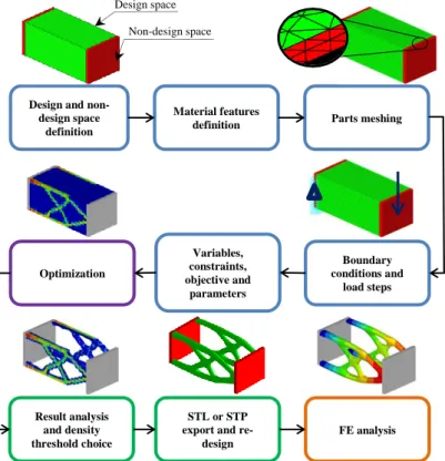
According to (Pradel et al., 2018), during the design process for additive manufacturing, one step must be the structure optimization. Applying the SIMP model - used throughout this article - with a commercial software (Optistruct from Altair) implies following the workflow detailed in Figure 1.
For (Rodrigue & Rivette, 2010), the design space (DS) is the volume in which the material can be assigned during the optimization. (Tang & Zhao, 2014) defined the design space as the
volumes which are used to bind the functional shapes and assist them in fulfilling their functional roles. As advised by (Goelke, 2016), the DS should be the largest one, allowing “to explore leading into the most design improvement opportunities”.
Functional shapes (FS) are defined as surfaces which can fulfill some functional requests (Tang & Zhao, 2014). They can be surfaces needed for connecting joints, or where loads are applied. A non-design space (NDS), even though part of the optimization problem, will not be modified during the optimization (Altair University, 2015). The use of NDS is optional when performing the optimization. NDS is:
used to give volume to functional shapes,
used to represent standard parts like bearings or the minimum thickness of fluid channels. The DS and optional NDS are integrated into the optimization software. Boundary conditions, load steps (defined for each stage of the part or of the product life), the material, optimization objective and constraints are defined to obtain the material density distribution.
The TO result, which is a density distribution, has to be interpreted. Thus, some parameters have to be chosen by the designers (M.-H. Hsu & Hsu, 2005; Y.-L. Hsu et al., 2001) leading to a particular result (Morretton et al., 2019). The parameters are, for example, the design space definition, the density threshold, or the penalty factor.
Figure 1. Traditional topology optimization workflow
Numerous articles or industrial applications illustrate design for AM by exploiting TO. For example (Tomlin & Meyer, 2011) demonstrated that different DS and NDS lead to different design and mechanical behaviour of a bracket. (Walton & Moztarzadeh, 2017) realized an optimised rear upright manufactured by electron beam melting. More recently (Munk et al., 2019) used topology optimization to find the minimum weight structures for a land gear.
Topological optimization of a multi-component product
As previously said, most of the AM articles have been written about the design of a single part (Barbieri et al., 2017; Han, 2017; Hodonou et al., 2019; Mancuso et al., 2019; Munk et al., 2019; Obaton et al., 2015; Ren & Galjaard, 2015; Tomlin & Meyer, 2011; Walton & Moztarzadeh, 2017), whereas the design optimization of additively manufactured multi-component products has rarely been studied. (Rodrigue & Rivette, 2010) designed a planetary gear system. After a step of parts consolidation, a topological optimization was carried out on each rigid body. The purpose of the study conducted by (Sossou et al., 2018) was to manufacture additively a non-assembly topologically optimized vice. The necessary clearance and the most adapted orientation were chosen before applying a TO on each part. (Orquéra et al., 2017) studied a multi-component system (an oscillating cylinder engine). The goal of this study was to functionally improve the engine by using AM capabilities. To achieve this, TO was applied on each component together with functional improvements of the joints.
Design and non-design space
definition
Material features
definition Parts meshing
Boundary conditions and load steps Variables, constraints, objective and parameters Result analysis and density threshold choice STL or STP export and
re-design
FE analysis Optimization
Design space Non-design space
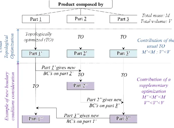
Figure 2. Comparison between one usual TO and multiple TO considering new BC on a multi-component design
Generally, mechanical systems are products whose parts have relative motions. Some parts and connecting joints undergo inertia loads. Topological optimization of moving parts allows to lightweight them and thus to reduce the loads due to inertia. For example, in the Figure 2, the part 1’ which is the topologically optimized part 1, gives new boundary conditions (BC) on the part 2’. So, part 2’ may be lighter with a new TO. The so optimized part denoted 2’’ has an impact on the BC of the optimized part 3’ which can be optimized again, and so on.
In light of this clearly observable research gap, the purpose of this article is to consider mass and inertia decrease in the designing of an optimized multi-component product.
Method
Optimization paths
The first step of the method is to determine the first part or set of parts that has to be optimized. As this optimization sequence planning may influence the design, different optimization paths have to be identified and compared according to certain criteria.
The criteria would correspond to data relative to the mechanical behaviour (denoted Mb) of the system. It can be, for example, the mass of the system. For a pump or a propulsion system, the input or output torque may be the selected data. Following this general idea, different
optimization paths can be identified, directly linked to the chosen criteria or not, as for instance: Path 1- The part whose inertia (or mass) has the greatest impact on the mechanical behaviour is optimized first,
Path 2- Beginning the optimization with the part that has a parameter involved in the highest number of equations related to the mechanical behaviour,
Path 3- All parts are optimized simultaneously,
Path 5- The part that has the most connecting joints to the other parts of the system is optimized first.
To determine which part has the greatest impact on the feature Mb, the reduced sensibility coefficient S* (Petit & Maillet, 2008) is used as shown in the Equation (3).
S∗(𝑀
𝑏/𝐶𝑖) = 𝐶𝑖.𝜕𝑀∂ 𝐶𝑏
𝑖 Equation (3)
Mb represents the mechanical feature and Ci the characteristic of the part i. The part whose characteristic leads to maximize S∗(𝑀
𝑏/𝐶𝑖) is optimised first for the Path 1.
For the Path 2, the static or dynamic mechanical equations have to be written in order to determine which part has a parameter involved in the highest number of equations. For the Path 5, connecting joints have to be counted.
In a next section three paths and two derivate one are applied to a case study in order to estimate the influence of the path choice.
Optimization impact estimation
The optimization impact estimation consists of estimating the need for a new topological
optimization. For instance, in the Figure 2, the product has an output torque T0. After the first TO the new torque is T1. If both torques are identical or almost identical, further optimization is not useful. On the contrary if they are not identical, a new TO is necessary. An important issue is to decide from which T1 value should a new TO be realized.
For this purpose, the mechanical behaviour ratio (denoted RMb) is proposed and calculated according to Equation (4).
𝑅𝑀𝑏 =𝑀𝑏𝐿−1
𝑀𝑏𝐿 Equation (4)
𝑀𝑏𝐿−1 and 𝑀𝑏𝐿 are the respective values of the mechanical behaviour criteria, previously chosen
by the designer, before and after the optimization. L (for loop) corresponds to the number of the considered TO loops. A parameter ε called convergence coefficient is also established. If the result of the RMb ratio is lower than 1-ε or higher than 1+ε, the impact is estimated as significant. So, new iterations have to be done while the mechanical ratio does not belong to [1-ε, 1+ε]. The lower ε is, the more the impact of TO on the mechanical behaviour is taken into account. But this will influence the number of loops and therefore the calculation time. In this article, the impact of the ε value is discussed based on a case study.
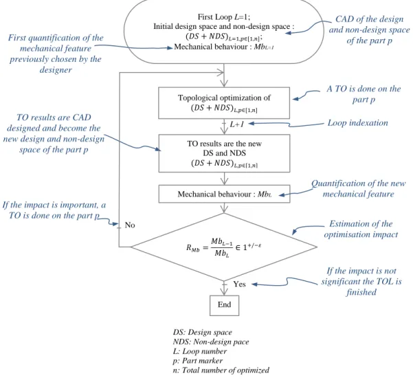
Figure 3. Topological optimization loop (TOL) organization chart considering inertia and mass decrease
The topological optimization loop
Based on the previous explanations, a organization chart showing the concept of Topological Optimisation Loop (TOL) for a multi-component is proposed in Figure 3.
Depending on the path choice, the TOL is applied first on the part which should be first optimised (for paths 1, 2 and 5), or on all the parts simultaneously for the path 3.
As explained in the topology optimization workflow (Figure 1), a design space and an optional non-design space are CAD designed for each “p” part and integrated into the optimization software. They are denoted by (𝐷𝑆 + 𝑁𝐷𝑆)𝐿=1,𝑝𝜖[1,𝑛] for the first loop. L and n are respectively
the loop and the part number. Boundary conditions, load steps, material, optimization objective and constraints are also initially defined.
The first loop is a classic application of the topological optimization (using the TO workflow shown in Figure 1). The result is a material density distribution. After interpretation, a new CAD-design of the part is used as the design space (with the same non-design space as before, as explained in a next section) for the next loop. Denoted (𝐷𝑆 + 𝑁𝐷𝑆)𝐿=2,𝑝∈[1,𝑛] , it now has a new
mass and inertia which impact the other parts.
As explained previously, if the result of the RMb ratio is lower than 1-ε or higher than 1+ε, the impact is estimated as significant. So, new iterations have to be done. Although this new
organization chart is helpful to optimize a multi-component product, it should be noted that it has to be applied part by part.
DS: Design space NDS: Non-design pace L: Loop number p: Part marker
n: Total number of optimized parts
CAD of the design and non-design space
of the part p First quantification of the
mechanical feature previously chosen by the
designer
Estimation of the optimisation impact If the impact is important, a
TO is done on the part p TO results are CAD designed and become the new design and non-design
space of the part p
Loop indexation
If the impact is not significant the TOL is
finished
Mechanical behaviour : MbL (𝐷𝑆 + 𝑁𝐷𝑆)𝐿,𝑝∈[1,𝑛] TO results are the new
DS and NDS 𝑅𝑀𝑏= 𝑀𝑏𝐿−1 𝑀𝑏𝐿 ∈ 1 +/−𝜀 End (𝐷𝑆 + 𝑁𝐷𝑆)𝐿,𝑝∈[1,𝑛] Topological optimization of Yes No L+1 First Loop L=1;
Initial design space and non-design space : (𝐷𝑆 + 𝑁𝐷𝑆)𝐿=1,𝑝∈[1,𝑛]; Mechanical behaviour : MbL=1
Quantification of the new mechanical feature
A TO is done on the part p
Discussion about the design space
Generally the design space is chosen as the least restrictive to allow the software to find the optimum solution. So, normally the DS volume has to be the largest one. At the end of the first loop of the TO, as explained before, the mass and inertia are decreased so the loads intensities are smaller than those of the first TO loop. A second TO has to be done in which two DS may be used:
the result of the first loop,
the initial design space.
In order to allow more possibilities for the software, it seems wise to impose the new boundary conditions on the initial design space. But, because the loads are lower, using the initial design space leads to a mass higher than using the DS re-designed from the previous TO result, as shown in Figure 4.
Figure 4. Impact of the design space choice for the second loop
The algorithm decreases the mass and verifies if the constraints are violated or not, until they are validated (see Figure 4). Moreover, if the first optimization loop gives a density distribution result under consequent loads, this same result will necessarily withstand the new lower loads. So using the DS of the previous loop has a great probability of converging with a lower mass and a shorter calculation time.
In conclusion, for the first TO the design space should be the least restrictive as possible. Then, for the next loops, using the previous DS with lower loads achieves better results.
Optimization path principle for the designers
Each path will lead to a specific result with a CPU time, a total mass, an estimation of the
mechanical feature, etc. The main purpose of this article is, based on the paths results, to suggest optimization path principles in order to help designers to choose the best path considering their design objective.
Hence, in the next section different paths, using the TOL, are applied to a case study in order to make some comparisons, to assess the improvement of the system (thanks to the presented method) and to conclude on the optimization path principle.
Case study
System presentation
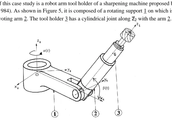
The subject of this case study is a robot arm tool holder of a sharpening machine proposed by (Bône et al., 1984). As shown in Figure 5, it is composed of a rotating support 1 on which is mounted a pivoting arm 2. The tool holder 3 has a cylindrical joint along z2 with the arm 2.
Figure 5. Case study: robot arm (Bône et al., 1984)
In order to simplify and target the objectives of the study, the following assumptions are made: friction and thermal effects are not considered.
In this study, only one case, placing the robot in a rather critical case is considered. The position of the arm 2 is constant and equal to 𝛽 = 0 rad. The study data are:
The rotating support has an acceleration equal to 𝛼̈(𝑡) =𝜋6 rad/s²,
Acceleration (and brake) inertia value are considered at t = 2 s,
The distances HG and OH are equal to 0.2 m and the tool rotation speed is equal to zero,
All parts are in common steel (Young modulus E = 210000 MPa; density = 7.8 kg/dm3; Poisson ratio = 0.3; Rpe = 210 MPa),
A safety factor is applied (s = 2).
Design spaces and non-design spaces were CAD designed for each part, as shown in Figure 6. The total mass of the non-optimized robot is equal to 16.2 kg and needs a torque to turn around z0 equal to 634 N.mm.
Figure 6. (a) Robot arm CAD designed; (b) Support; (c), Pivoting arm; (d) Tool. Design spaces are in green, and non-design spaces in orange.
(t) 𝛼(𝑡)
Cross-sections of each part with loads and boundary conditions are shown in Figure 7.
Figure 7. Boundary conditions applied on (a) Part 1, (b) Part 2, (c) Part 3
Paths identification
During its work, the robotic structure is permanently subjected to several types of loads like the grinding forces, or the inertial forces of moving masses (Mejri et al., 2016). The deflections of the structure under these loads are a source of defects for the grinding work that should be minimized. That is why the objective of this study is to use the TOL in order to reduce inertia. Three optimization paths are first proposed:
(1) The part whose inertia (or mass) has the greatest impact on the mechanical behaviour is optimized first.
(2) Beginning the TOL with the part that has a parameter involved in the highest number of equations.
(3) All parts are optimized simultaneously.
The input torque T01 (see Equation (8) in the appendix) is chosen to be the mechanical behaviour
data Mb used for the comparison of the several optimization paths.
The mathematical model used is proposed by (Bône et al., 1984). Tij and Fij represent
respectively the torque and the force between part i and part j. Ip(L,m) depicts the inertia of part p
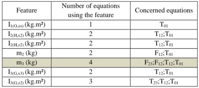
at point L around the axle m. All the equations are located in the appendix. As shown in Table 1, the component 3 impacts the highest number of equations.
The input torque (see Equation (8) in the appendix) has been evaluated for initial characteristics. To determine which part has the highest impact, the reduced sensibility coefficient S* of the Equation (3) is determined for each characteristic as shown in Table 2. The mass of arm 2 has the most important influence on the torque T01.
Table 1. Feature which impacts the highest number of mechanical equations
Feature Number of equations
using the feature Concerned equations
I1(O,zo) (kg.m²) 1 T01 I2(H,x2) (kg.m²) 2 T12;T01 I2(H,z2) (kg.m²) 2 T12;T01 m2 (kg) 2 F12;T01 m3 (kg) 4 F23;F12;T12;T01 I3(G,x3) (kg.m²) 2 T12;T01 I3(G,z2) (kg.m²) 3 T23;T12;T01
Table 2. Inertia and mass sensibility evaluation
Characteristic Ci m2 m3 I1(O ,z o) I2(H ,x2) I2(H ,z 2) S∗(𝑇 01/𝐶𝑖) = 𝐶𝑖. 𝜕T01 ∂ 𝐶𝑖 0.34 0.21 0.03 0.05 0.03 (a) (b) Fmass/zo Finertia/x1 A B Fmass/zo Finertia/z2 F32 C Finertia/y1 Finertia/y1 Fmass/zo Finertia/z2 Finertia/y1 (c)
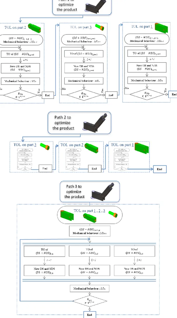
To summarize, the first Path begins with part 2, and the second Path 2 with part 3. Figure 8 graphically summarizes the three paths.
For this study, the convergence coefficient ε is imposed at 0.1. The results are compared in terms of robot total mass, input torque T01, and time used by the software to perform all the topological
optimization iterations.
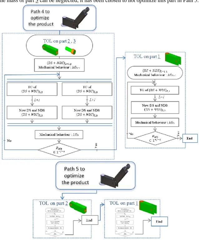
Other paths can be derived from these first three, like the two other possibilities shown in Figure 9. Path 4 is inspired from both Path 1 and Path 2, and consists in applying the TOL on parts 2 and 3 simultaneously and then on part 1.
As the mass of part 3 can be neglected, it has been chosen to not optimize this part in Path 5.
Details of the topological optimization paths
The topological optimization and CAD software used are respectively Optistruct and Inspire from Altair.
For each component, the TO objective is to minimize the mass with stress and displacement constraints. A static displacement constraint has been defined at points A, B and C for each part (the points are visible in Figure 7). This total displacement must not exceed 0.3 mm. For parts 1 and 2, (x1, zo) is used as a symmetric plane (the axle is visible in the Figure 5). The tool holder 3
turns around the axle z2. As the loads follow the same direction, a circular repetition around the
axle (7 repetitions) has been imposed.
It was determined to set the optimization parameters to 3 for the penalty factor and 6 for the related sensitivity filter called “mindim”. The mesh size is equal to 2 mm (except for part 3 due to its smaller size, where the mesh size is equal to 1 mm).
Finally, all the topological optimizations were performed on the same cluster. It is composed of two processors Xeon E5-2690/v2, each using ten cores of 25 Mo L3 with a frequency equal to 3 GHz. The RAM memory is equal to 256 Go.
Path 1: beginning with the most influential part (part 2)
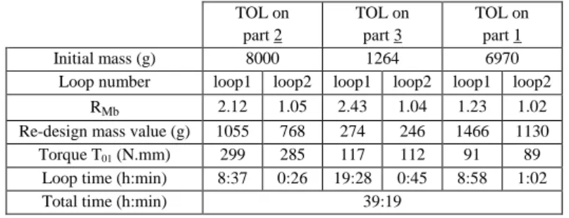
The results are summarized in Table 3.
Table 3. Optimization results for Path 1 TOL on part 2 TOL on part 3 TOL on part 1 Initial mass (g) 8000 1264 6970
Loop number loop1 loop2 loop1 loop2 loop1 loop2
RMb 2.12 1.05 2.43 1.04 1.23 1.02
Re-design mass value (g) 1055 768 274 246 1466 1130 Torque T01 (N.mm) 299 285 117 112 91 89
Loop time (h:min) 8:37 0:26 19:28 0:45 8:58 1:02
Total time (h:min) 39:19
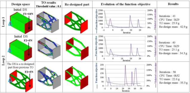
TOL on part 2
The first loop has converged and all constraints have been satisfied after 44 iterations. With the initial design space, the input torque T01 is equal to 634 N.mm. The first optimization loop
decreases this value to 299 N.mm. The resulting ratio equal to 2.12 has exceeded the limits specified in the previous section. So, a new loop is performed.
As explained previously, the design space used for the second loop is the result of the first loop. The second loop has converged and all constraints have been satisfied after 39 iterations. The ratio between the previous and new mechanical behaviour, equal to 1.05, is within the limits specified in the previous section. The optimization loops for part 2 have thus been finished. It can be noted that the re-design mass value is 12% less than the re-design mass value result with the initial design space, confirming the conclusions of the previous section. Then, new loads induced by mass and inertia of part 2 at the end of loop 2 are mandatory for the TOL of part 3.
TOL on part 3
The first loop generates a ratio RMb equal to 2.43, which is beyond the limits. The ratio of the
second loop remains within the limits.
The ratio RMb required two loops to be within the limits.
Path 2: beginning with the component which impacts the highest quantity of equations (part 3)
All optimization loops have converged and all constraints have been satisfied. Taking into account the mechanical behaviour ratio, each part has required two loops, as shown in Table 4. For each part, the design space obtained after the first loop is used for the second loop.
Table 4. Optimization results for path 2 TOL on part 3 TOL on part 2 TOL on part 1 Initial mass (g) 1264 8000 6970
Loop number loop1 loop2 loop1 loop2 loop1 loop2
RMb 1.36 1.01 3.84 1.08 1.23 1.04
Re-design mass value (g) 274 246 926 749 1434 912 Torque T01 (N.mm) 466 461 120 112 91 88
Loop time (h:min) 19:28 0:45 10:20 0:32 7:48 1:09
Total time (h:min) 40:04
Path 3: all parts simultaneously optimized
The results of Path 3 are summarized in Table 5. To obtain a value of RMb within the boundaries,
three loops are necessary.
Table 5. Optimization results for path 3 Initial Loop 1 Loop 2 Loop 3
RMb 5.74 1.20 1.07
TOL on part 1. Mass (g) 6970 1616 1287 1133 TOL on part 2. Mass (g) 8000 1055 801 735 TOL on part 3. Mass (g) 1264 274 246 234 Torque T01 (N.mm) 634 110 92 86
Total time (h:min) 20:54
Results analysis
Comparison of the results
As presented before, the results are different for each path. Figure 10 shows the re-designed products for each path and the results are summarized and compared in Table 6.
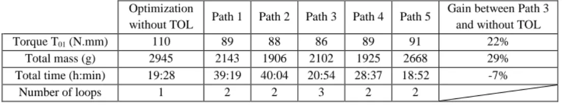
Without the TOL proposed previously, only one TO loop would have been performed. To verify the gains made by performing TOL, Table 6 shows the differences between a single topological optimization and the TOL results. Results prove that TOL produces significant gains in mass compared with one TO loop, and this, within the same amount of time in both instances.
Table 6. Results of each path and comparison between using a single topological optimization and using the TOL
Optimization
without TOL Path 1 Path 2 Path 3 Path 4 Path 5
Gain between Path 3 and without TOL
Torque T01 (N.mm) 110 89 88 86 89 91 22%
Total mass (g) 2945 2143 1906 2102 1925 2668 29%
Total time (h:min) 19:28 39:19 40:04 20:54 28:37 18:52 -7%
Figure 10. Robot arm optimized using the TOL for each path
It can be noted that the complex shapes of the robot arm so obtained cannot be manufactured by conventional processes. Using the Analytic Hierarchy Process (AHP) method proposed by (Mançanares et al., 2015), a powder bed fusion (PBF) process should be used as the most adapted AM process.
The total time is lower for Path 3 compared with Paths 1 and 2. Indeed, as the parts have been simultaneously optimized, the total CPU time is not the sum of the software time for each part optimization, but the sum of the maximum CPU time for each loop, as explained in Figure 11.
Figure 11. Comparison of the CPU times for the different paths
About the convergence coefficient ε
The convergence coefficient used for this case study is equal to 0.1. This means that the TOL scheme is ended if the mechanical behaviour of the new loop exceeds plus or minus 10% of the
P
at
h
1
Part 1 Part 2 Part 3
P at h 2 P at h 3
Total time of the path 1: ~39h Path 1 B eg in n in g o f th e p at h En d o f th e p at h TOL on part 3 TOL on part 1
TLi: Time of the loop i TOL on part 2
TL1 TL2
TL1 TL2
TL1 TL2
Total time of the path 2: ~40h Path 2 B eg in n in g o f th e p at h En d o f th e p at h TOL on part 1 TOL on part 3 TL1 TL2 TL1 TL2
Total time of the path 3: ~21h Path 3 B eg in n in g o f th e p at h En d o f th e p at h First loop Part 2 Part 3 Part 1 Second loop Third loop TOL on part 2 TL1 TL2
previous one. The results of the different paths show that this value is wise and gives good results with few iterations.
Choosing a convergence coefficient close to zero will drastically increase the quantity of loops without effective results. Moreover, the low decrease in loads during the next iterations will reduce the potential gain at each new iteration.
On the contrary, choosing a high coefficient of convergence will reduce the quantity of loops, but the results may not be optimum. For example, using ε equal to 0.3 for the third path leads to only two loops (Table 7) but with a total robot mass increased by 11%. Likewise, the input torque has increased by 7%. In return, there is only a 3% savings in time.
Table 7. Impact of the convergence coefficient for Path 3
Path 3 ε=0.3 ε=0.1 ε=0.05
Torque T01 (N.mm) 92 86 85
Total mass (g) 2334 2102 2051
Total time (h:min) 20:15 20:54 21:05
Number of loops 2 3 4
Figure 12 shows changes in the total mass and the RMb ratio as a function of the loop number for the path 3. The lower ε is, the more the RMb and the total mass tend towards an asymptotic (RMb=1 in orange on the graph in Figure 12). However, there is a significant gain when the slope is high. In conclusion, it is necessary to choose a reasonable value of ε to obtain a significant gain without loss of time. Thus it seems that the convergence coefficient should be included in the range [0.1; 0.2].
Figure 12. Mass and RMb evolution as a function of the number of loops for the Path 3
Principles to select a path for an additively manufactured multi-component product optimization
Each path has led to different results. Considering the designer objectives, the choice of the path can be different. A classification of the paths is suggested in Table 8.
First, it can be noticed that Path 1 has nearly no advantage. On the contrary, Path 3 seems to have the best numbers, especially to lead to the lowest input torque. Path 4 has one tenth of a gram more than Path 2; this is low enough to equalize them. Both enable the greatest decrease in mass. Lastly, if saving time is the primary objective, Path 5 has to be used.
0 1 2 3 4 5 6 7 0 2 4 6 8 10 12 14 16 18 0 1 2 3 4 R a ti o R Mb T o ta l m a ss (k g ) Loop number Result for ε=0,3 Result for ε=0,1 Result for ε=0,05 RMb=1
Table 8. Ranking of the paths considering the objectives of the designer The objective is to reduce the
mass torque time
Path 1 3 3 4
Path 2 1 2 5
Path 3 2 1 2
Path 4 1 3 3
Path 5 4 4 1
1 represents the best path, 5 represents the worst.
Thanks to these results, the most effective path can be chosen to achieve the designer objectives. For this reason, three optimization principles can be concluded (for mechanisms without a closed-loop kinematic chain and to minimize the mass with stress as objective and displacement as constraints):
(1) To optimize a product with a minimum use of time:
The part(s) with the least influence on the mechanical behaviour must not be optimized.
The most influential part has to be optimized first.
(2) To optimize a product in order to obtain the best mechanical behaviour:
All parts which impact the mechanical behaviour have to be optimized simultaneously. (3) To optimize a product in order to obtain the lowest mass:
The part whose mass is involved in the highest number of equations has to be optimized first.
To reduce the length of time, the heaviest parts can be optimized simultaneously.
Conclusion
The case study presented in this article has resulted in the design of an optimized robot arm. More generally, the topological optimization loop (TOL) concept proposed in this article takes into account the decrease in mass and inertia during the topological optimization of a mechanical product. Even if the topology of the results may differ a little, the presented method is not
software dependent. Indeed, the TO loop can be applied in the same way and the conclusions will be identical.
To perform an optimization on a multi-component product, the topological optimizations may be applied on the parts in different orders. Several optimization paths have been tested, leading to different results. Finally, for the case study examined in this report, using the TOL framework together with the best optimization path leads to an additional 35% gain in mass in comparison with a single topological optimization. Integrating the TOL framework in a Design for Additive Manufacturing (DfAM) method, will provide a rational and helpful tool for obtaining a
mechanical system in which:
material savings is achieved,
the mass is lower,
the dynamic behaviour is better,
the joints between rigid bodies withstand lower loads,
The choice of the design space for the successive optimization loops has also been studied. Using the density distribution result of the previous loop as the new design space seems to improve the results.
Finally, as the choice of the path must be made to achieve the designer objectives, three
optimization principles have been stated, depending on the objective: minimizing the calculation time, obtaining the best mechanical behaviour or obtaining the lowest mass. Thus, following these recommendations will help designers to optimize a multi-component product.
The presented method is a convenient tool to design static or dynamic systems. However, it must be used for multi-component products in which mass and inertia have an impact on the
mechanical behaviour. To complete this research, future work should focus on studying complex systems with closed-loop kinematic chains. Another perspective could be to conduct a similar study for other TO objectives and constraints.
Appendix
In this section the equations used for the case study are detailed. As explained previously, the mathematical model used is proposed by (Bône et al., 1984). Tij and Fij represent respectively the
torque and the force applied between part i and part j. Ip(L,m) depicts inertia of part p at point L
around axis m (Figure 5).
(𝑥⃗0, 𝑥⃗1) = (𝑦⃗0, 𝑦⃗1) = 𝛼 Equation (5) (𝑧⃗0, 𝑧⃗2) = (𝑥⃗1, 𝑥⃗2) = 𝛽 Equation (6) (𝑥⃗2, 𝑥⃗3) = (𝑦⃗1, 𝑦⃗3) = 𝛾 Equation (7) 𝑇01= 𝑑𝑡𝑑 [{𝐼1(𝑂,𝑧⃗0)+ (𝐼2(𝐻,𝑥⃗2)+ 𝐼3(𝐺,𝑥⃗3)). 𝑠𝑖𝑛²𝛽 + (𝐼2(𝐻,𝑧⃗2)+ 𝐼3(𝐺,𝑧⃗2)). 𝑐𝑜𝑠²𝛽 + 𝑚2. ℎ² + 𝑚3. (ℎ + 𝑟. 𝑠𝑖𝑛𝛽)²}. 𝛼̇ + 𝐼3(𝐺,𝑧⃗2). 𝛾̇. 𝑐𝑜𝑠𝛽] Equation (8) 𝑇12 = (𝐼2(𝐻,𝑦⃗⃗2)+ 𝐼3(𝐺,𝑥⃗3)+ 𝑚3. 𝑟2). 𝛽̈ + {(𝐼 2(𝐻,𝑧⃗2)+ 𝐼3(𝐺,𝑧⃗2)− 𝐼2(𝐻,𝑥⃗2)− 𝐼3(𝐺,𝑥⃗3)). 𝛼̇. 𝑐𝑜𝑠𝛽 + 𝐼3(𝐺,𝑧⃗2). 𝛾̇}. 𝛼̇. 𝑠𝑖𝑛𝛽 − 𝑚3. 𝑟. [(ℎ + 𝑟. 𝑠𝑖𝑛𝛽). 𝛼̇2. 𝑐𝑜𝑠𝛽 + 𝑔. 𝑠𝑖𝑛𝛽] Equation (9) 𝑇23= 𝑑𝑡𝑑 [𝐼3(𝐺,𝑧⃗2). (𝛾̇ + 𝛼̇. 𝑐𝑜𝑠𝛽)] Equation (10) 𝐹23 = 𝑚3. [𝑔. 𝑐𝑜𝑠𝛽 − 𝑟. 𝛽̇2− (ℎ + 𝑟. 𝑠𝑖𝑛𝛽). 𝛼̇2. 𝑠𝑖𝑛𝛽] Equation (11) 𝐹21 = (𝛼̈. 𝑡)2. ℎ. (3.𝑚2 2 + 2. 𝑚3) Equation (12) 𝑂𝐻 ⃗⃗⃗⃗⃗⃗⃗ = ℎ. 𝑥⃗1 Equation (13) 𝐻𝐺 ⃗⃗⃗⃗⃗⃗⃗ = 𝑟. 𝑧⃗2 Equation (14)
h and r are constant.x
References
Altair University. (2015). Practical Aspects of Structural Optimization - A study guide. Aremu, A., Ashcroft, I., Hague, R., Wildman, R., & Tuck, C. (2010). Suitability of SIMP and
BESO Topology Optimization Algorithms for Additive Manufacture. Twenty First Annual
International Solid Freeform Fabrication Symposium, 679–692.
Barbieri, S. G., Giacopini, M., Mangeruga, V., & Mantovani, S. (2017). A design strategy based on topology optimization techniques for an additive manufactured high performance engine piston. Procedia Manufacturing, 11, 641–649.
Bendsøe, M. P. (1995). Optimization of Structural Topology, Shape, and Material.
Bendsøe, M. P., & Sigmund, O. (1999). Material interpolation schemes in topology optimization.
Archive of Applied Mechanics, 69(9–10), 635–654.
Bône, J.-C., Morel, J., & Boucher, M. (1984). Mécanique générale: cours et applications. Brackett, D., Ashcroft, I., & Hague, R. (2011). Topology optimization for additive
manufacturing. Proceedings of the Solid Freeform Fabrication Symposium, Austin, TX., 348–362.
Chu, S., Xiao, M., Gao, L., Li, H., Zhang, J., & Zhang, X. (2019). Topology optimization of multi-material structures with graded interfaces. Computer Methods in Applied Mechanics
and Engineering, 346, 1096–1117.
Eschenauer, H. A., & Olhoff, N. (2001). Topology optimization of continuum structures: A review. Applied Mechanics Reviews, 54(4), 331.
Goelke, M. (2016). 5 ways to rethink optimization.
Guo, X., & Cheng, G.-D. (2010). Recent development in structural design and optimization. Acta
Mechanica Sinica, 26(6), 807–823.
Hällgren, S., Pejryd, L., & Ekengren, J. (2016). (Re)Design for Additive Manufacturing.
Procedia CIRP, 50, 246–251.
Han, P. (2017). Additive design and manufacturing of jet engine parts. Engineering, 3(5), 648– 652.
Hodonou, C., Balazinski, M., Brochu, M., & Mascle, C. (2019). Material-design-process selection methodology for aircraft structural components: application to additive vs subtractive manufacturing processes. International Journal of Advanced Manufacturing
Technology, 1–9.
Hsu, M.-H., & Hsu, Y.-L. (2005). Interpreting three-dimensional structural topology optimization results. Computers and Structures, 83(4–5), 327–337.
Hsu, Y.-L., Hsu, M.-S., & Chen, C.-T. (2001). Interpreting results from topology optimization using density contours. Computers and Structures, 79(10), 1049–1058.
Kim, H., Querin, O. M., & Steven, G. P. (2002). On the development of structural optimization and its relevance in engineering design. Design Studies, 23(1), 85–102.
Krishna, L. S. R., Mahesh, N., & Sateesh, N. (2017). Topology optimization using solid isotropic material with penalization technique for additive manufacturing. Materials Today:
Proceedings, 4(2), 1414–1422.
Liu, J., Gaynor, A. T., Chen, S., Kang, Z., Suresh, K., Takezawa, A., … To, A. C. (2018). Current and future trends in topology optimization for additive manufacturing. Structural
and Multidisciplinary Optimization, 57(6), 2457–2483.
Additive manufacturing process selection based on parts’ selection criteria. The
International Journal of Advanced Manufacturing Technology, 80(5–8), 1007–1014.
Mancuso, A., Pitarresi, G., Saporito, A., & Tumino, D. (2019). Topological optimization of a structural naval component manufactured in FDM. Advances on Mechanics, Design
Engineering and Manufacturing II, 2, 451–462.
Mejri, S., Gagnol, V., Le, T. P., Sabourin, L., Ray, P., & Paultre, P. (2016). Dynamic characterization of machining robot and stability analysis. International Journal of
Advanced Manufacturing Technology, 82(1–4), 351–359.
Micheletti, S., Perotto, S., & Soli, L. (2019). Topology optimization driven by anisotropic mesh adaptation: Towards a free-form design. Computers and Structures, 214, 60–72.
Morretton, E., Vignat, F., Pourroy, F., & Marin, P. (2019). Impacts of the settings in a design for additive manufacturing process based on topological optimization. International Journal on
Interactive Design and Manufacturing (IJIDeM), 13(1), 295–308.
Munk, D. J., Auld, D. J., Steven, G. P., & Vio, G. A. (2019). On the benefits of applying topology optimization to structural design of aircraft components. Structural and
Multidisciplinary Optimization, 1–22.
Obaton, A.-F., Bernard, A., Taillandier, G., & Moschetta, J.-M. (2015). Fabrication additive : état de l ’ art et besoins métrologiques engendrés. Revue Française de Métrologie, 2015–
1(37), 21–36.
Orquéra, M., Campocasso, S., & Millet, D. (2017). Design for additive manufacturing method for a mechanical system downsizing. Procedia CIRP, 60, 223–228.
Petit, D., & Maillet, D. (2008). Techniques inverses et estimation de paramètres. Partie 1.
Techniques de l’ingénieur, 33, 1–18.
Ponche, R., Kerbrat, O., Mognol, P., & Hascoet, J. Y. (2014). A novel methodology of design for Additive Manufacturing applied to Additive Laser Manufacturing process. Robotics and
Computer-Integrated Manufacturing, 30(4), 389–398.
Pradel, P., Zhu, Z., Bibb, R., & Moultrie, J. (2018). A framework for mapping design for additive manufacturing knowledge for industrial and product design. Journal of
Engineering Design, 29(6), 291–326.
Ren, S., & Galjaard, S. (2015). Topology optimisation for steel structural design with additive manufacturing. In Modelling Behaviour (pp. 35–44). Springer Cham.
Rodrigue, H., & Rivette, M. (2010). An assembly-level design for additive manufacturing methodology. IDMME - Virtual Concept, 1–9.
Rozvany, G. I. N., Zhou, M., & Birker, T. (1992). Generalized shape optimization without homogenization. Structural Optimization, 4(3–4), 250–252.
Saadlaoui, Y., Milan, J. L., Rossi, J. M., & Chabrand, P. (2017). Topology optimization and additive manufacturing: Comparison of conception methods using industrial codes. Journal
of Manufacturing Systems, 43, 178–186.
Sossou, G., Demoly, F., Montavon, G., & Gomes, S. (2018). An additive manufacturing oriented design approach to mechanical assemblies. Journal of Computational Design and
Engineering, 5(1), 3–18.
manufacturing. ASME. ASME International Mechanical Engineering Congress and
Exposition, Volume 2B, V02BT02A030.
Tang, Y., & Zhao, Y. F. (2016). A survey of the design methods for additive manufacturing to improve functional performance. Rapid Prototyping Journal, 22(3), 569–590.
Thompson, M. K., Moroni, G., Vaneker, T., Fadel, G., Campbell, R. I., Gibson, I., Bernard, A., Schulz, J., Graf, P., Ahuja, B., & Martina, F. (2016). Design for additive manufacturing: trends, opportunities, considerations, and constraints. CIRP Annals - Manufacturing
Technology, 65, 737–760.
Tomlin, M., & Meyer, J. (2011). Topology optimization of an Additive Layer Manufactured (ALM) aerospace part. Proceeding of the 7th Altair CAE Technology Conference, 1–9. Vayre, B., Vignat, F., & Villeneuve, F. (2012). Designing for additive manufacturing. Procedia
CIRP, 3(1), 632–637.
Walton, D., & Moztarzadeh, H. (2017). Design and development of an additive manufactured component by topology optimisation. Procedia CIRP, 60, 205–210.
Zhang, Y., Xiao, M., Li, H., Gao, L., & Chu, S. (2018). Multiscale concurrent topology optimization for cellular structures with multiple microstructures based on ordered SIMP interpolation. Computational Materials Science, 155, 74–91.
Zhou, M., Pagaldipti, N., Thomas, H. L., & Shyy, Y. K. (2004). An integrated approach to topology, sizing, and shape optimization. Structural and Multidisciplinary Optimization,
26(5), 308–317.
Zhou, M., & Rozvany, G. I. N. (1991). The COC algorithm, Part II: Topological, geometrical and generalized shape optimization. Computer Methods in Applied Mechanics and