RESEARCH OUTPUTS / RÉSULTATS DE RECHERCHE
Author(s) - Auteur(s) :
Publication date - Date de publication :
Permanent link - Permalien :
Rights / License - Licence de droit d’auteur :
Bibliothèque Universitaire Moretus Plantin
Institutional Repository - Research Portal
Dépôt Institutionnel - Portail de la Recherche
researchportal.unamur.be
University of Namur
The influence of social network topology in a opinion dynamics model
Righi, Simone; Carletti, Timoteo
Publication date:
2009
Document Version
Early version, also known as pre-print
Link to publication
Citation for pulished version (HARVARD):
Righi, S & Carletti, T 2009, 'The influence of social network topology in a opinion dynamics model', Paper
presented at European Conference on Complex Systems 2009, Warwick, Angleterre, 21/09/09.
General rights
Copyright and moral rights for the publications made accessible in the public portal are retained by the authors and/or other copyright owners and it is a condition of accessing publications that users recognise and abide by the legal requirements associated with these rights. • Users may download and print one copy of any publication from the public portal for the purpose of private study or research. • You may not further distribute the material or use it for any profit-making activity or commercial gain
• You may freely distribute the URL identifying the publication in the public portal ? Take down policy
If you believe that this document breaches copyright please contact us providing details, and we will remove access to the work immediately and investigate your claim.
(will be inserted by the editor)
The influence of social network topology in a opinion
dynamics model
Simone Righi · Timoteo Carletti
Received: date / Accepted: date
Abstract We investigate an opinion dynamics model with continuously defined affini-ties and opinions. We focus here on the effects of the social network’s topology on the dynamical evolution and on the scale properties of the model measured through nu-merical simulations and fittings. We study different network topologies through a set of statistical network measures, namely mean path, mean degree and clustering. We observe that the model’s dynamics eventually leads to a uniformization of the different topologies.
Keywords sociophysics; opinion dynamics; agent based model; group interactions, networks
1 A model of Opinion Dynamics
We hereafter describe and analyze a model of opinion dynamics, already introduced and discussed in [1,4,5] in which binary interactions are considered. We call this model
α-model. We consider a population made of N fixed agents, i.e. a closed group setting;
each agent is characterized by its opinion on a given subject, here represented by a real number Oi∈ [0, 1], and moreover each agent possesses an affinity with respect to
any other, αij ∈ [0, 1], the higher is αij the more affine, friend, the agents are and
consequently behave. Thus affinity and opinion are continuous variables. In this paper we focus on the effects of the initial distributions of the first variable on the evolution of the system. In this context the affinities αij∀i, j ∈ N is used in order to build a
matrix α that describes the underlying social network.
Around these 2 variables we now can detail the dynamics of the model. At each time step an agent m is randomly selected in the population with an uniform proba-Simone Righi
D´epartement de Math´ematique,
Facult´es Universitaires Notre-Dame de la Paix Namur, Belgium, 5000
Tel.: +32-(0)81-724933 Fax: +32-(0)81-724914
bility. Then another agent n is chosen: it is the one who minimizes the social metric constructed as the product between the distance from the opinion of m and the affinity with it. The concept of social temperature is introduced, in the selection of the second agent, with the introduction of a normally distributed stochastic component with mean 0 and variance σ. n is thus the agent selected though the formula:
n = arg£min((1 − αt−1mj)|Ot−1j − Ot−1m |) + N (0, σ) ¤
∀j ∈ N : j 6= m (1) where the agent m (already selected) is obviously excluded from the equation.
Each agent changes its opinion toward the average opinion of the couple if it is affine enough toward the other. Otherwise its opinion remains unchanged. The measure of the affinity needed for the opinion’s convergence is given by the parameter αc(fixed to
0.5 for all the simulation of this paper). Mathematically the updating of the opinions is described by the equations:
Ot+1m = Otm+ µtanh(ζ(α t mn− αc)) + 1 2 (O t n− Otm) (2) and Ont+1= Ont+ µtanh(ζ(α t nm− αc)) + 1 2 (O t m− Ont) (3)
where µ is a convergence parameter fixed to 0.5 for all the simulations adopting the viewpoint of [9] that states that the value of this parameters does not to affect the dynamics and the behavior of the system but only the time that the system takes to go on equilibrium. ζ is a parameter, set to 1000, used in order to transform numerically the function tanh in a step function.
The updating of the affinities αmnand αnmis similarly described by the equations:
αt+1mn = αtmn+ (1 − αtmn)αtmn ¡
− tanh£ζ(|∆Otmn| − ∆Oc) ¤¢
(4) and
αt+1nm = αtnm+ (1 − αtnm)αtnm ¡
− tanh£ζ(|∆Otmn| − ∆Oc) ¤¢
(5) where ∆Oc- set to 0.50 - is the threshold that defines the updating of the affinities
(i.e the affinities increase if |∆Onm| < ∆Oc, while decrease if |∆Onm| > ∆Oc).
This model has been introduced in [1] and it’s affinity’s networks has been studied in [5] along the following research directions:
1. Distribution of the values of the main network variables; 2. Evolution of the main network parameters in time;
3. Evolution of the main network parameters with respect to different numbers of agents.
In this paper we move away from the simplifying assumption of randomness for the network of the affinities, implementing more sophisticated network initializations, with the aim of studying situations where the initial topology is more similar to the reality of the social environment.
We present here the results of some numerical simulations where the initial topology of α is:
1. a random network in which the number of active links are distributed uniformly random [1],[7];
2. a scale free network created through the Barab´asi-Albert preferential attachment dynamics [2]. We study in detail this topology in section 3 analyzing its evolution both temporal and with the size of the model for scale free with different slopes γ. To observe the perseverance this kind of distribution of the degrees in the network we also present the time evolution of the degree distribution;
3. a small world network created though the relinking process described by Watts and Strogatz [8]. We study this topology in section 4;
4. a regular lattice in which to each agent is assigned a fixed number of connections. We are here interested to observe the evolution of the networks’ statistical features and in particular to understand if through the dynamics its characteristics are preserved in time. This means, for the scale free initialization to verify if the initial distribution of the degrees remains a power-law before the convergence of the opinions and for the small world one, if the network continue to have a big clustering contextually to a small average mean path.
Finally (section 5) we compare all the different initializations proposed above look-ing before to the temporal evolution of the networks statistical measures as the dy-namics evolve the opinions toward the convergence and then to the characteristics of these measures when the opinions converged, variating the system’s population size.
2 Network statistical measures
As anticipated in this paper we focus on the study of the topological characteristics of the model’s networks to do so we observe that the affinity matrix α can be considered an adjacency matrix. Since every couple of agents m,n has, by definition, an affinity greater than 0, in principle all the relationships are active, but since only the connections with high values are really significative, we decided to consider as ’active links’ those that exceed a value αf set to 0.25 for the simulation on the Bar´abasi-Albert distributions
of section 3 and to 0.50 in all the other simulations. The reason for this is difference is that in the former case we need to know the initial distribution of the degrees. In all the cases, infact, an active affinity is initialized at 0.375 while a non-active one to 0.125. With this choice we want to clearly separate the two possible initial states. For the network analysis we thus binarize the matrix α according the threshold αfcreating
the adjacency matrix a. The values on the diagonal of the matrix are set to zero at the begin of the simulation and they are never modified by the dynamics, it is thus impossible for misleading 1-loop (which could lead to impossible self-iterations) to be created.
In order to study networks with high numbers of vertices and dense interconnec-tions, we use four standard - broadly accepted - statistical measures calculated on the whole network i.e.: the mean degree (< k >) of the vertices, the mean path (< l >) between vertices and the clustering (< C >) of the network. In order to obtain a con-nected network, i.e. to provide finite values for the mean path, we set the parameters so that the dynamics lead to a consensus - i.e. only one cluster in opinion space - among the agents.
3 Barab´asi-Albert Scale Free Initialization
We begin studying the evolution of the α-model when the affinities matrix is initialized as a scale free network `a la Barab´asi and Albert. The initial degrees of the agents will be therefore distributed accordingly to a power-law with a slope γ (see the different slopes in the two left panes of figure 2).
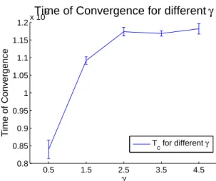
For the following simulations the number of agents is fixed to 350 a value that allows the presence of an appreciable difference between the hubs and the other nodes. In all the cases anyway the more a scale free initialization is steep the more slowly is the model to converge (see figure 1). This phenomena can be explained observing that a steeper scale-free means that, proportionally, many nodes have a relatively small degree at the beginning of the simulation, leading - caeteris paribus - to a longer transient before the interaction becomes effective and lead to convergence in the opinion space.
0.5 1.5 2.5 3.5 4.5 0.8 0.85 0.9 0.95 1 1.05 1.1 1.15 1.2x 10 5 γ Time of Convergence
Time of Convergence for different
γ
Tc for different γ
Fig. 1 Time of convergence Tcfor different slopes of γ. All the results are referred to sets of
10 simulation with 350 agents, the affinities matrix initialized as a scale free network, σ=0.5,
αc=0.5 and with ∆Oc= 0.5.
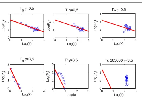
In figure 2 we observe that the dynamics disrupt the scale free distribution of the nodes, and that at the convergence of the opinions it is lost. We can anyway observe that this happen more slowly for small γ’s with respect to the high γ’s. One possible explanation for this difference is that as the slope of the initial distribution increases the nodes with few connections (the leafs) are proportionally in greater number, with respect to the hubs; therefore the former are selected more often than the latter and they have greater chances of getting more connected (i.e. increasing their degree). When
γ is small at the opposite there is no substantial difference between the hubs and the
leaves of the network and therefore the relatively larger connectivity of the former keep the distribution stable longer. Our system is of limited dimensions but it is possible to say that for an initialization with a power-law with a slope larger than 2 the transient becomes progressively shorter with respect to the time of convergence of the opinions, while for γ < 2 the transient becomes very long and we can say that the original type of degree’s distribution is maintained.
0 1 2 3 0 1 2 3 Log(k) Log(P k ) T 0γ=0,5 0 1 2 3 0 1 2 3 Log(k) Log(P k ) T’ γ=0,5 0 1 2 3 0 1 2 3 Log(k) Log(P k ) Tc γ=0,5 0 1 2 3 0 1 2 3 Log(k) Log(P k ) T 0γ=3,5 0 1 2 3 0 1 2 3 Log(k) Log(P k ) T’ γ=3,5 0 1 2 3 0 1 2 3 Log(k) Log(P k ) Tc 105000 γ=3,5
Fig. 2 Evolution of the degree’s distribution in 2 generic simulations with the affinity matrix initialized as a scale-free network with respectively γ = 0.5 (upper panels) and γ = 3.5 (lower panels). The distributions are referred to simulations with 350 agents, σ=0.5, αc=0.5 and with
∆Oc= 0.5. For all the figures αf=0.25 The red lines are the best fit of the initial distribution
and have slope -0.5 and -3.5 in accordingly with the correspondent values of γ. The first panels on the left represent the k distribution at the beginning at the simulation, the second column represent the moment in which the initial distribution significatively variates from a power law distribution (this happens at T ≈ 30000 for γ = 0.5 and already at T ≈ 5000 for γ = 3, 5), finally the right column’s panels shows the distribution of the k when the convergence is reached (T ≈ 80000 for γ = 0.5 and T ≈ 105000 for γ = 3.5).
Observing the figure 3 we can also observe that the slope of the power law to which we initialize the system has a declining effect on the dynamics as it increase (notice the differences between the trends at γ = 0.5 and γ = 1.5 in particular for the mean path and the mean degree) its influence decay very fast. This effect is mainly due to the limited size of the networks studied with this model but it would appear, at higher
γ even scaling up the model. The growth of the mean degree during the simulation is
very slow reaching, at convergence, only 0.5 in the best case, and it takes a longer time to be reached with respect to the case of a random initialization of the network. The growth follows, for the different γ, a behaviour which can be best fitted as:
< d >=Atb A b R2 γ = 0.5 7.75 10−3 0.89 0.99 γ = 1.5 6.11 10−4 1.36 1 γ = 2.5 1.41 10−4 1.64 0.99 γ = 3.5 1.15 10−4 1.68 0.99 γ = 4.5 1.09 10−4 1.69 1
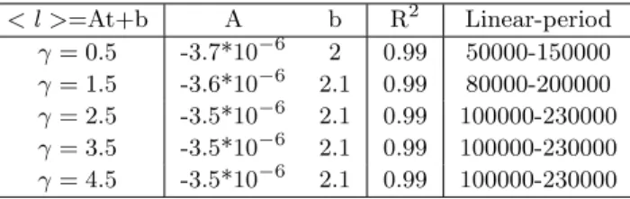
The mean path in Fig. 3 shows that the lower the slope of the scale free the lower is the initial mean path (at which the network becomes connected) and consequently
the evolution of the variable is slowlier than in the case in which γ is higher. The trend is initally exponential, then it assumes a linear behaviour during which the opinions converge. The characteristics of this linear period period can be summarized as:
< l >=At+b A b R2 Linear-period γ = 0.5 -3.7*10−6 2 0.99 50000-150000 γ = 1.5 -3.6*10−6 2.1 0.99 80000-200000 γ = 2.5 -3.5*10−6 2.1 0.99 100000-230000 γ = 3.5 -3.5*10−6 2.1 0.99 100000-230000 γ = 4.5 -3.5*10−6 2.1 0.99 100000-230000
Since the mean path has a lower bound at 1 this trend cannot be continuous. We can infact observe, at the end of the simulation a cut off after which the system converge to one.
Finally the network clustering increases in a relevant way during the simulation, while γ does not seems to have a relevant effect on the characteristics of the trend if not in the steps before the convergence where the different initial slopes leads, temporarily to different patterns of growth.
0 2 4 6 8 10 12 x 104 0 0.1 0.2 0.3 0.4 0.5 0.6 0.7 Steps
Normalized Mean Degree
Mean Degree for different γ
γ=0.5 γ=1.5 γ=2.5 γ=3.5 γ=4.5 0 2 4 6 8 10 12 x 104 1 1.5 2 2.5 3 3.5 Steps Mean path
Mean Path for different γ
γ=0.5 γ=1.5 γ=2.5 γ=3.5 γ=4.5 0 2 4 6 8 10 12 x 104 0 0.1 0.2 0.3 0.4 0.5 0.6 0.7 0.8 Steps
Normalized network clustering
Network Clustering for different γ
γ=0.5
γ=1.5
γ=2.5
γ=3.5
γ=4.5
Fig. 3 Dynamic evolution of the main networks measures for different slopes γ. All the trends are referred to sets of 10 simulation with 350 agents, the affinities matrix initialized as a scale free network, σ=0.5, αc=0.5 and with ∆Oc= 0.5.
All this hints lead us to think that the scale free distribution in the mean degree is preserved, to some degree, at least in the first steps of the simulation. This depends
from the fact that the nodes with more connections tend to preserve their special status thought the simulation, working as hubs in the creation of the convergence. However after a transitory phase the differences in degree among the agents eventually decline and the network connectivity lose the memory of its initialization. This is due to the partner-selection mechanism of our model. As seen in equation 1 the selection of the ’partner’ for the interactions depends on both the difference in opinions |Ojt−1− Ot−1m |
and the affinity αt−1mj. At the beginning of the simulation the difference in terms of affinities between hubs and leaves of a scale free distribution is negligible. On the contrary the number of leaves, expecially when γ is large, greatly outnumbers the number of hubs. Therefore the leaves are more likely to be selected since they lay on average at a relatively shorter distance from the node m. Let’s imagine, as an example a scale-free network with 3 highly connected hubs and 347 poorly connected leaves. The leaves have an average distance (in opinions) from the selected agent of 1/347, while the tree hubs are distant, on average 1/3. The former are therefore much more often selected as ’partners’ than the latter, increasing therefore their relative degree.
As the population grows (see figure 4) also the time to achieve a convergence and the mean path at which this happen grows. At the opposite the larger the population the lower, on average, the number of acquaintances of each agent (as shown by the values of mean degree and clustering). The time of convergence and the value of mean path and clustering at convergence increase with the slope of the power-law at which the model is initialized. At the opposite the mean degree is lower for higher values of
γ for all the system sizes analyzed. This can be interpreted as a residual effect of the
presence of hubs in a scale free initialization. As the networks become larger the hubs tend to be more markedly separated, in terms of degree of initialization, from the other nodes. Therefore even when the distribution of the nodes becomes bell-shaped it will always have a relatively fat right tail. That leads to the convergence in more time but with a structure of network with less connections (as more agents has less opportunities to interact due to the relative attractivity of the ’ex-hub’ as partner the creation of new active connections is comparatively less likely). This relative attractivity increase with the size of the model producing the pattern observed for mean path and network clustering in figure 4.
4 Watts-Strogatz initial distribution
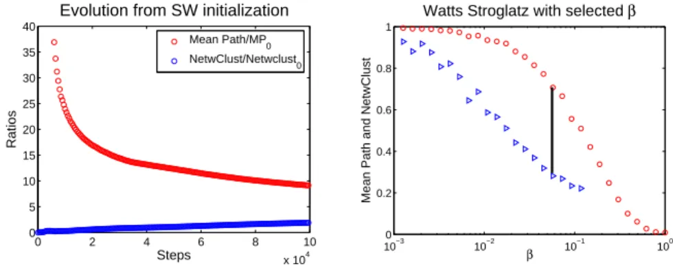
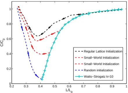
Watts and Strogatz proposed in [8] a mechanism to create small world networks, which begins with the construction of a regular lattice, in which every node has k neighbor. Then with a probability β each of the edges is re-linked. It is possible to apply this technique to create a ‘small world’ network to be used as initialization of our model. In our case we select networks with k=4 and k=10 (each agents has 4 or 10 initial connections) and we iterate the procedure described by Watts and Strogatz to find which is the probability β that maximize the distance between the clustering and the mean path of the network (the procedure is schematized in the right panel of figure 5). Then we proceed to evolve this setup with the rules of the α-model. The result is represented in the left panel of figure 5, where in order to understand if the network remains small world we observe the behaviour of network clustering and mean path in comparison with their initial value (which is small world as seen on the right part of the figure). We can clearly observe that as the model evolves the network of the affinities keeps the characteristics of a small world network: the mean path tends to
0 100 200 300 400 0 2 4 6 8 10 12x 10 4 Number of Agents Time of Converngence
Time of Convergence vs N for different γ
γ=0.5 γ=1.5 γ=2.5 γ=3.5 γ=4.5 0 100 200 300 400 0.2 0.3 0.4 0.5 0.6 0.7 Number of agents
Normalized Mean Degree
Mean Degree vs N for different γ
γ=0.5 γ=1.5 γ=2.5 γ=3.5 γ=4.5 0 100 200 300 400 1.3 1.4 1.5 1.6 1.7 Number of agents Mean Path
Mean Path vs N for different γ
γ=0.5 γ=1.5 γ=2.5 γ=3.5 γ=4.5 0 100 200 300 400 0.1 0.2 0.3 0.4 0.5 0.6 0.7 0.8 Number of agents
Normalized Network Clustering
Network Clustering vs N for different γ
γ=0.5 γ=1.5 γ=2.5 γ=3.5 γ=4.5
Fig. 4 Evolution of the networks measures at convergence for different slope γ . All the trends are referred to sets of 10 simulation with the affinities matrix initialized as a scale free network, with σ=0.5, αc=0.5 and with ∆Oc= 0.5.
decrease and the network clustering to growth. This is what we expect in the case of the persistence of the initial network. The behaviour observed is confirmed if we look
0 2 4 6 8 10 x 104 0 5 10 15 20 25 30 35 40 Steps Ratios
Evolution from SW initialization
Mean Path/MP0 NetwClust/Netwclust0 10−3 10−2 10−1 100 0 0.2 0.4 0.6 0.8 1 β
Mean Path and NetwClust
Watts Stroglatz with selected β
Fig. 5 Time evolution of network clustering and mean path with respect to the ones of the initialization Watts and Strogatz small world in a simulation with k=4 and N=200 (left image) and the corresponding Watts and Strogatz graph with indicated the β selected for the initialization which maximize the distance between the two variables (right image).
the Watts-Strogatz rule representation where the curves of mean path and clustering are plotted removing the dependence from β. In this way we are able to show, on the same graph the evolution of these two topological measures and observing if the models remains small world or not. Clearly all the measures are still normalized with respect to the one of the regular lattice from which we start for the creation of the network. As we see, whichever the initial β is, the model evolutions increase the connectivity in a way that seems to preserve a small world structure.
0.2 0.3 0.4 0.5 0.6 0.7 0.8 0.9 1 0 0.2 0.4 0.6 0.8 1 L/L 0 C/C 0
Regular Lattice Initialization Small−World Initialization Small−World Initialization Random initialization Watts−Strogatz k=10
Fig. 6 Clustering and mean path (normalized with respect to the one of a regular lattice) for k=10 (solid azure line). The figure represent the two variables plotted one against the other. The dynamical evolution of simulations, whose affinity matrix is initialized using different levels of β (dashed lines), shows that as the simulation evolves the network keeps it’s small world initialization while increasing the connectivity. In red the simulations that starts from a small world set of parameters, in blue the one initialized as a almost-random and in violet a simulation initialized as almost a regular lattice.
5 Comparison of different initializations
In this section we compare the dynamical evolution of the α- model when the affinity matrix is initialized with the topologies presented in the previous sections.
In the specific to initialize the small world we use the same parameters and proce-dure described in section 4. In the case of the scale free we use a γ = 2.5 which seems to represent a reasonable choice (as shown in section 3 this value seems to share the same evolution characteristics, with reference to our model, that other similar values). For regular lattices we fix a number of connections per agents (four in the simulations presented here) and we produce a regular topology with that number of connections.
The connectivity is used also to initialize the random networks, with the difference that in this case the connectivity of each agent is randomly distributed and only the average si preserved.
5.1 Evolution in time
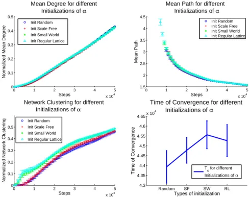
Figure 7 clearly shows that the evolutions when we start with different initializations produce very similar patterns, in particular with respect to the mean degree and the mean paths. For both of them we can outline a single best fit for all the initializa-tions: < k > (All Distributions) ≈ 1.2 ∗ 10−3t1.51 and < l > (All Distributions) ≈ 7905t−0.8951+1. On the contrary we observe small but observable differences among the dynamical evolutions of the network clusterings which can be explained if we consider that the different topologies presents different degrees of clustering with the regular lattice and small world characteristically having a larger one than the scale free and random networks. This difference is maintained during the first part of the simulation then it tends to disappear. The trends are complex and not immediately fitting any trivial function, but they show a remarkable similarity.
For what regards the dynamical evolution we can therefore conclude that the α-model is indifferent to the topology of the affinities’ network.
0 1 2 3 4 5 x 10⁴ 0 0.1 0.2 0.3 0.4 0.5 Steps
Normalized Mean Degree
Mean Degree for different Initializations of α
Init Random Init Scale Free Init Small World Init Regular Lattice
0 1 2 3 4 5 x 10⁴ 1.5 2 2.5 3 3.5 4 4.5 Steps Mean Path
Mean Path for different Initializations of α
Init Random Init Scale Free Init Small World Init Regular Lattice
0 1 2 3 4 5 x 10⁴ 0 0.1 0.2 0.3 0.4 0.5 Steps
Normalized Network Clustering
Network Clustering for different Initializations of α
Init Random Init Scale Free Init Small World Init Regular Lattice
Random SF SW RL 4.3 4.35 4.4 4.45 4.5 4.55 4.6 4.65x 10 4 Types of initialization Time of Convergence
Time of Convergence for different Initializations of α
T
c for different
Initializations of α
Fig. 7 Dynamical evolution of the main network measures for different initializations. All the trends are referred to sets of 10 simulations with σ=0.5, αc=0.5 and with ∆Oc= 0.5. The last
image represent the average and the standard deviation of the time of convergence for different initializations of the affinity matrix (α).
5.2 Evolution with the size of the model
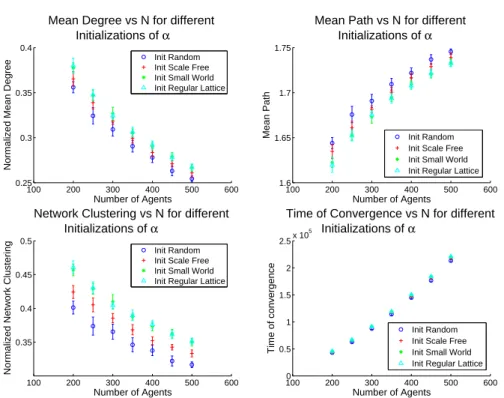
In this section we propose a comparative study of the convergence results under differ-ent types of α topologies as the size of the model grows. As for the dynamical evolution also in this case we observe (figure 8) that when the size of the model, i.e. the number of agents used, changes we can still observe very similar pattern for all the types of topologies used. We can fit the pattern of evolution of the variables with the following laws (the law presented are an average of the results of the different initializations whose difference are not significative):
y=ANb A b R2 y=< d > 1.54 -0.37 0.97 y=< l > 1.06 0.07 0.96 y=< C > 1.32 -0.28 0.97 y=Tc 1.93 1.73 0.98
From these fits it is clear that the networks statistics will continue their trend for big values of the number of agents (N), but the boundaries embedded in the networks (the degree and the clustering can’t be smaller than 0, the mean path not larger than N), suggest the existence of an cut-off of this laws for large population of agents. While the trends are essentially equal we can observe some difference in the values of the network measures at which the different initializations topologies converges. These differences allow us to observe that the less regular network tends to converge with a smaller average degree, a larger average path and a smaller network clustering, we must observe anyway that, in particular for the mean degree and the mean path, they are not significative, being the error bars largely overlapped. Figure 8 also confirms that the dynamics of α-model tends to eliminate the initial differences that we introduced with the different initializations since the different affinity’s networks look statistically very similar when the opinions converge.
6 Conclusions
Opinion dynamics models with continuous opinions attracted considerable attention in the last years. We introduced in this paper a variation on the model with affini-ties presented in [1,4,5] studying the effects of different topologies of social (affinity) networks on the evolution of the model. We have shown, through fits and numerical simulations that the dynamical evolution of the model tends to homogenize the topol-ogy of the network eliminating the statistical difference introduced in the initialization phase. We studied with particular attention the cases in which the affinities are ini-tialized as scale free and small world networks. While the former initialization lose its characteristic trait during the evolution (the power law distribution), the latter one is resilient and survive to the dynamics of the model.
In general we can state that, in our simplified environment the topology of the social network on the base of which the agents interact does not change significatively the dynamics of the model which, supposing the presence of individual with a suffi-ciently big willingness to listen different opinions (i.e. a suffisuffi-ciently big αc), leads to a
100 200 300 400 500 600 0.25 0.3 0.35 0.4 Number of Agents
Normalized Mean Degree
Mean Degree vs N for different Initializations of α
Init Random Init Scale Free Init Small World Init Regular Lattice
100 200 300 400 500 600 1.6 1.65 1.7 1.75 Number of Agents Mean Path
Mean Path vs N for different Initializations of α
Init Random Init Scale Free Init Small World Init Regular Lattice
100 200 300 400 500 600 0.35 0.4 0.45 0.5 Number of Agents
Normalized Network Clustering
Network Clustering vs N for different Initializations of α
Init Random Init Scale Free Init Small World Init Regular Lattice
100 200 300 400 500 600 0 0.5 1 1.5 2 2.5x 10 5 Number of Agents Time of convergence
Time of Convergence vs N for different Initializations of α
Init Random Init Scale Free Init Small World Init Regular Lattice
Fig. 8 Evolution the main network measures at the convergence of the opinions as its size (N) change, for different initial topologies. All the trends are referred to sets of 10 simulations with
σ=0.5, αc=0.5 and with ∆Oc= 0.5. The last image represent the average and the standard
deviation of the time of convergence for the different topologies of the affinity matrix (α) as they evolve with the size of the model.
Despite that we found that under some condition is possible to create networks which are more resient to change. For the case of scale free initialization we observed that the slope of the initial degree distribution makes a relevant difference for the time in which it is maintained during the dynamics. While for the small world initialization we discovered that the fundamental characteristics of this kind of network (high network clustering associated with low mean path) are not destroyed by the dynamics.
We provided growth laws which allow to predict the model results when the model is applied at larger scales or longer evolution times. Interestingly most of the trends are best fitted by a power law, suggesting the presence of some kind of scale invari-ance with respect to the affinity’s topological measures. On this regard we shown that despite strong similarities in the convergences times, the networks with more ordered structure (i.e. regular lattices and small worlds) tends to converge with larger average degrees and clusterings and with smaller mean paths than the networks with a less or-dered organization (random and scale free), as it is expected to happen the real world dynamics. Finally we observed that, while the presence of hubs in the initial network does not change significatively the final shape of the social network the uniformization effect of the model’s dynamics is stronger when the slope of the power law with which we initialized the model is larger.
References
1. F. Bagnoli et al.: Dynamical affinity in opinion dynamics modeling, PRE, 76, pp.066105, (2007).
2. A.-L. Barab´asi,; R. Albert: Emergence of scaling in random networks, Science, 286, pp. 509512,(1999).
3. T. Carletti et al.: How to make an efficient propaganda, Europhys. Lett., 74 (2), pp. 222-228, (2006).
4. T. Carletti et al.: Birth and death in a continuous opinion dynamics model. The consensus
case, Volume 64, Number 2, pp.285-292, (2008).
5. T. Carletti, On the evolution of a social network, preprint, (2009).
6. T. Carletti et al.: Shaping opinions in a social network, Accepted for Proceedings of Italian
Workshop of Artificial Life and Evolutive Computation, (2008).
7. P. Erd¨os; A. R´enyi On Random Graphs I, Publicationes Mathematicae, 6, pp. 290-297, (1959).
8. D.J. Watts, S.H. Strogatz: Collective dynamics of small-world networks”, Nature, 393, pp 440, (1998).
9. G. Weisbuch, G. Deffuant, et al: Meet, Discuss and Segregate!, Complexity, 7, No. 3, (2002). 10. E.M. Jin, Michelle Girvan, M.E.J. Newman: ”The Structure of Growing Social Networks,”,