HAL Id: hal-01897058
https://hal-amu.archives-ouvertes.fr/hal-01897058
Submitted on 30 Apr 2020
HAL is a multi-disciplinary open access
archive for the deposit and dissemination of
sci-entific research documents, whether they are
pub-lished or not. The documents may come from
teaching and research institutions in France or
abroad, or from public or private research centers.
L’archive ouverte pluridisciplinaire HAL, est
destinée au dépôt et à la diffusion de documents
scientifiques de niveau recherche, publiés ou non,
émanant des établissements d’enseignement et de
recherche français ou étrangers, des laboratoires
publics ou privés.
Country factors and the investment decision-making
process of sovereign wealth funds
Jeanne Amar, B. Candelon, C. Lecourt, Z. Xun
To cite this version:
Jeanne Amar, B. Candelon, C. Lecourt, Z. Xun. Country factors and the investment
decision-making process of sovereign wealth funds.
Economic Modelling, Elsevier, 2019, 80, pp.34-48.
Country
factors and the investment decision-making process of sovereign
wealth
funds
☆
J.
Amar
a, B. Candelon
b,c, C.
Lecourt
d, Z. Xun
e,*a Aix-Marseille University, CERGAM EA 4225, France bUniversité Catholique de Louvain, Belgium
cMaastricht University, The Netherlands d Aix-Marseille University, AMSE, France
e School of Economics, Jiangxi University of Finance and Economics, China
JEL classification: C33 C35 E61 G23 F39 G3 Keywords:
Sovereign wealth funds Targeted countries
Macroeconomic country factors Two-tiered dynamic Tobit panel model
A B S T R A C T
In this paper, we examine the complex decision-making processes that lead to sovereign wealth funds’ (SWFs’) choice of investment location. Using a two-tiered dynamic Tobit panel model, we find that country-level factors do not have the same impacts on the investment decision and the amount to invest and that SWFs tend to invest more frequently and at higher amounts in countries in which they have already invested. More specifically, we find that SWFs prefer to invest in countries with higher political stability, whereas they are more prone to invest large amounts in countries that are less democratic and more financially open. Our results also lend support to the idea that SWFs are prudent in their choice of a target country with regard to their investment decision but behave as more opportunistic investors with regard to the amounts to be invested.
1. Introduction
Sovereign wealth funds (SWFs), ”government-owned investment funds set up for a variety a macroeconomic purposes” (IMF (2008)), have received increasing attention since the late 2000s. Many countries have established SWFs for various macroeconomic purposes, such as stabi-lization, saving for future generations or investments in long-term eco-nomic projects (such as infrastructure or education). The assets man-aged by these funds, which are estimated at 7.3 trillion by the Sovereign Wealth Funds Institute in June 2017, have grown tremendously over the past decade, driven by high oil prices and current account surpluses, particularly in Asia. While the size and rapid growth of SWFs suggest that these funds have become major players in the finance world, buy-ing large stakes in companies and givbuy-ing governments exposure to
sec-☆The authors are grateful for the comments and remarks received at the AFFI, Infiniti and the internal seminars at the University of Liège. Bertrand Candelon conducted this study with the research program “Risk Management, Investment Strategies and Financial Stability” under the aegis of the Europlace Institute of Finance and Insti7. The usual disclaimer applies.
* Corresponding author.
E-mail addresses:[email protected](J. Amar),[email protected](B. Candelon),[email protected](C. Lecourt),decxun@hotmail.
tors they may otherwise be unable to access, their objectives and behav-ior are not well understood. In particular, the opaqueness surrounding their structure and activities appear to be a major concern in host coun-tries, for which it is unclear whether SWFs behave like governments or like institutional investors.
With the rapid expansion of sovereign wealth funds, financial economists have attempted to better understand the decisions made by this new class of investors. This task is not easy, as many SWFs are particularly opaque regarding their objectives and functioning. In addition, their investment decision-making process is complex because it combines several dimensions that can potentially inter-act. One of the main questions regarding SWFs’ investment strategy is how they select countries and companies in which they invest. Are their investment strategies based only on financial motives, or
are they also founded on macroeconomic, political or institutional considerations?
Most studies generally attempt to identify the main factors driving SWFs’ investment decisions. Some papers assess whether these factors are macroeconomic (Ciarlone and Miceli (2014), Knill et al. (2012), or Megginson et al. (2013)) or political (Bernstein et al. (2013), Knill et al. (2012)). Other empirical studies also stress the link between the characteristics of the fund, such as its size, its degree of opacity, the origin of the funding (commodity versus non-commodity) and its investment decision (Knill et al. (2012), Avendano (2012), Meggin-son et al. (2013)). These studies conclude that SWFs’ investments are influenced by the characteristics of the SWF and by those of the target countries.
Another dimension of SWFs’ investment decision-making process is the way they invest. In what type of firms will they prefer to invest, and what amount? Existing empirical studies dealing with this dimension have generally focused on the financial characteristics of the firm (for example, the firm’s size and risk) as determinants of SWFs’ investment strategy (see, for example, Kotter and Lel (2011)). In the same spirit,
Johan et al. (2013) attempt to measure the choice of SWFs for investing in public versus private global firms and show that SWFs are more likely to invest in private firms in countries that have less-developed legal systems.
In line with this existing literature, the aim of this paper is to bet-ter understand the decision-making process that leads to the choice of investment locations by this new class of investors. More specifi-cally, we attempt to explain SWFs’ motivation to invest in a particular country by considering the geographic, economic, political and insti-tutional distances between the acquiring and target countries. Using a new database for the recent period 2000–2014, we examine 609 foreign equity investments made by 29 SWFs from 15 countries in 72 target countries. Based on the recent paper by Xun and Lubrano (2016), we adopt a sophisticated two-tiered dynamic panel Tobit model to jointly estimate the decision to invest and the amounts to be invested. The dynamic dimension in the panel model allows us to estimate whether SWFs tend to invest more frequently and at higher amounts in countries in which they already have invested.
Anticipating on our findings, we find that SWFs’ investments are driven by country-level factors. This paper also shows that the deter-minants of the investment decision are different from those driving the amount of investment, motivating the use of the two-tiered Tobit panel model to investigate this issue. In particular, our results lend support to the idea that SWFs are prudent in the choice of target country with regard to their investment decision but behave as more opportunistic investors with regard to the amounts to be invested. Ultimately, our findings exhibit a persistence in SWF investment strategy, which means that SWFs have a tendency to invest again in the target country once the decision to invest has been taken.
The paper is organized as follows. Section 2 introduces the theoreti-cal framework and the hypotheses for analyzing SWFs’ investment deci-sions abroad. Section 3 provides details on the data. Section 4 presents the econometric methodology, Section 5 reports our empirical findings, and Section 6 concludes.
2. Theoretical framework and empirical hypotheses
Extensive recent literature investigates the potential factors driving SWF investment decisions. In particular, because they are state-owned investment funds that may be managed either by the ministry of finance or by a board composed of government officials, SWFs’ investment strat-egy may be not only commercially oriented but also politically biased. We report this literature and show how it opens pathways for new research on the identification of SWFs’ investment determinants. H1. SWFs tend to invest in countries that share the same macroeconomic,
geographical, political and institutional characteristics as the home country.
Most of the literature studying SWFs addresses the main concern raised by these investors: is SWFs’ investment strategy guided by purely financial motives, or is it biased by more strategic objectives? In order to answer this question, a large section of the literature has attempted to identify the main drivers of SWF investments.
Even if certain authors show that firm-level characteristics influence SWFs’ investment decisions (see, among others,Kotter and Lel (2011)
orAvendano (2012)), a large portion of the literature shows that SWFs’ investment decisions are driven mostly by country factors. More specif-ically, relying on the literature on Foreign Direct Investments (FDI), certain papers test whether SWFs are more likely to invest in countries that are similar to their home countries in terms of culture, economic development or political institutions.Chhaochharia and Laeven (2009)
andMegginson et al. (2013)show that SWFs prefer to invest in coun-tries with which they share the same culture (in terms of language or religion). For other variables, results are more divergent.Megginson et al. (2013)find that SWFs are more prone to invest in countries that are trade partners, whereasChhaochharia and Laeven (2009)find opposing results.Knill et al. (2012)show that SWFs prefer to invest in countries that are close (in terms of geographic distance), whileMegginson et al. (2013)find that geographic proximity does not explain SWFs’ invest-ment decisions. Finally,Knill et al. (2012)conclude that SWFs are more likely to invest in countries with which they have weak political bilat-eral relations.
Although the existing literature finds evidence that country factors matter in SWFs’ investment decision-making process, there is a lack of consensus regarding the determinants of their investment strategy. The great heterogeneity among SWFs, the unavailability of data on some of their transactions and specification problems can explain the variation in these results.
Relying on the empirical literature on Foreign Direct Investments (FDIs) (see, among others,Anderson and Van Wincoop (2003),Stulz and Williamson (2003)andKang and Kim (2008)), we expect that SWFs will prefer to invest in regions or countries in which they have either an information advantage or perceived familiarity in terms of cultural, institutional or macroeconomic characteristics.
In the same way, we predict that geographic proximity will be asso-ciated with more investment deals between both countries.
H2. Target country factors do not have the same impacts on the investment
decision and the amount to invest.
Note thatH1does not provide information on the way SWFs will invest. Once the decision of whether or not to invest in a given country has been made based on country-level factors, SWFs decide the amount to be invested. In line withKnill et al. (2012), we consider SWFs’ com-plex decision-making process by specifying two stages. In the first stage, the SWF chooses the country in which it will invest. In the second stage, the SWF decides how much it will invest. Ignoring the two-stage nature of the investment decision assumes that country factors have the same impact during both stages. We expect that country-level factors’ impact on the investment decision differs from that on the amount of the invest-ment.
H3. SWFs tend to invest more frequently and at higher amounts in countries
in which they have already invested.
Related toH1, if a SWF chooses to invest in a country that shares similar characteristics in terms of macroeconomic, political, institu-tional or cultural factors, it will likely continue to invest in this country in the future because it is already informed about this target country. In this way, it avoids search and informational costs of investing in this country. Therefore, we test whether there is a learning effect in the SWF investment decision-making process. If so, once an investment decision is taken, the SWF will likely keep investing in the same country in the future.
3. Data and descriptive analysis
3.1. The SWF sample
In both the academic and the practitioner literature, there is no con-sensus on exactly what an SWF is. A unanimously accepted definition is that given by the International Monetary Fund (IMF (2008)), according to which “SWFs are government-owned investment funds established for a variety a macroeconomic purposes”. Considering the lack of consensus on the definition of an SWF and the lack of transparency in the method-ologies used in the existing empirical literature to collect data, we have decided to construct a unique database from scratch using the following methodology.1
Considering this definition, we conducted a search of all existing SWFs by using different sources in order to have the most complete list. We begin with a preliminary sample of SWFs given on the SWF Insti-tute website2by combining the names of funds published by JP Morgan (Fernandez and Eschweiler (2008)),Catalano (2009),Lyons (2007)and the SWFs’ websites. When different names for the same SWF are found, we employ the fund’s websites to eliminate duplicates. Moreover, we consider a fund to be active if it has made at least one publicly reported investment internationally. Because many funds have been created and announced on the websites but are not active, this search yields a sam-ple of 89 existing SWFs in 2013, but only 29 of these funds from 15 countries are retained for the analysis.3Details on these 29 funds are presented inAppendix 1.
3.2. Investment data
We construct our sample of SWFs’ investments in listed firms using two different sources. First, we search the financial database Thomson Reuters Eikon Mergers and Acquisitions for all known SWFs and their subsidiaries in order to identify transactions involving SWFs. Second, we use the online database Factiva to complete the missing acquisi-tions. Investment data are extracted for both the SWFs and their wholly owned subsidiaries.4 The features of each transaction are collected: information about the targeted firms (name and country), information about the SWFs (name, subsidiary, and country), the date of the trans-action, the pre- and post-acquisition shares of the investment in the target firm and the value of the deal.
Table 1presents summary statistics – overall and by year – for the number and total value of cross-border SWF deals. The combined sam-ple for both sources from 2000 to 2013 allows us to capture 609 cross-border acquisitions by 29 SWFs with a total value of USD 278,406 million.5 As described in Table 1, SWFs made an increasing num-ber of cross-border investments between 2005 and 2007, driven by fast-growing influxes of revenue combined with the search for bet-ter returns. The number of cross-border investments reached a peak in 2007, with 118 investments representing approximately 19% of the
1For example, the Sovereign Investor Institute’s Sovereign Wealth Center
includes 32 funds in its database, whereas the SWF Institute retains 78 SWFs.
2http://www.swfinstitute.org/.
3Because our analysis focuses on the investment amounts, we retain only
cross-border transactions for which the deal value is available.
4The newswires cited above report information regarding the name of the
fund, the name of the subsidiary, the name of the target firm and the size of the stake.
5Through open market share purchases, Norway’s Government Pension Fund
Global (GPFG) acquired many small stakes in listed companies during the con-sidered period (more than 55,000 investments with a stake size of less than 2%). For this reason, we choose to remove it from the database. All the invest-ments and their market value are given by Norway’s Government Pension Fund Global on its website:http://www.nbim.no/en/Investments/holdings.
total number of foreign transactions over the 2000–2013 period.6 Dur-ing the crisis, many funds shifted their investment strategies, retreatDur-ing from foreign markets and increasing their domestic investments. The number of foreign investments sharply dropped in 2008, even though the volume of investment activity remained substantially high (the total value of SWF investments in 2008 represents 21.1% of the total value of SWF investments over the 2000–2013 period). In the past few years, SWFs have continued to actively invest abroad, with 136 transactions completed in 2012–2013.
Table 2presents the distribution of cross-border investments made by SWFs of 15 countries in terms of their value and number and shows that the majority of the most active SWFs are located in Asia and in the Middle East. Singapore made more cross-border investments than any other country (265 foreign deals, which represents 43.5% of all SWF investments by number and 36.07% by value), followed by SWFs from the United Arab Emirates (21.8% of deals, 30.8% of value),7Qatar (14.3% of deals, 12.07% of value) and China (7.1% of deals, 12.4% of value). We observe that funds from Kuwait made few investments compared to the others (2.3% of deals) but did so at large amounts (4.43% of all investments by value).
Finally,Table 3outlines the geographical distribution of SWF coun-try investments by number (Panel A) and by value (Panel B) in target firm regions. The clear trend revealed by this table is SWFs’ prefer-ence to invest in the developed countries of North America (18.23% of total deals, 27.63% of value) and Western Europe (26.6% of total deals, 32.91% of value), particularly in the English common law countries of Canada, the United States and Great Britain. This trend is clearly the case for SWFs from the United Arab Emirates, Qatar, China and, to a lesser extent, Singapore, which have invested (in number and in value) in both regions over this period. The other target regions are the Far East (14.78% of total deals, 9.33% of value) and the Indian Subconti-nent (13.63% of total deals, 6.12% of value). The fact that the majority of SWF investments are targeted towards developed countries with safe institutions, high revenues and financial regulations reveal that macroe-conomic factors matter for their investment decisions. Less clearly, this picture reveals a tendency for SWFs to invest in their own geographi-cal region. More precisely, SWFs from the Middle East and South Asia also prefer to invest in their own geographical region even if they seem to have a strategy of geographical diversification. Note that geograph-ical diversification of SWF cross-border investments is sometimes very different in number and in amounts, which suggests that the SWF deci-sion to invest in a particular country and the decideci-sion regarding the amount to invest in this country are not based on the same criteria. A revealing example is the only stake in Central and South America purchased by the fund of Qatar amounted to an impressive USD 2716 million.8
4. Methodology: the two-tiered dynamic Tobit panel model In this paper, we estimate a two-tiered dynamic Tobit panel model developed by Chang (2011b) and improved by Xun and Lubrano (2016). The choice of this model offers many advantages to better evaluate the decision-making process that leads to SWFs’ investment location. First, the “two-tiered” dimension allows a distinction between the decision to invest and how much the SWF invests. Second, the SWF decision to invest in a particular country may also be persistent over time. It means that if a first investment has been made in year
6In 2007, SWFs emerged as major players on the world financial markets; in
particular, they pumped USD 60 billion into Western banks during the financial meltdown.
7The Abu Dhabi Investment Authority (ADIA) is considered the second
biggest fund.
8Qatar Holding invested USD 2716 million in Banco Santander Brazil, which
represents 5% of stakes. 3
Table 1
Annual distribution of SWFs’ foreign investments. This table presents the number of deals and the total deal value of cross-border investments led by
SWFs (excluding Norway) by year. Column 3 provides the proportion of the number of SWF investments made in year t among all investments made over the 2000–2013 period. Column 5 shows the proportion of the value of SWF investments made in year t among the total value of SWFs’ foreign
investments over the 2000–2013 period.
Year Number of foreign investments Proportion (Number of deals) Total value of foreign investments (USD million) Proportion (Amount)
2000 17 2.8% 3665.9 1.3% 2001 4 0.7% 9260.7 3.3% 2002 8 1.3% 898.9 0.3% 2003 13 2.1% 2713.3 1.0% 2004 13 2.1% 5108 1.8% 2005 42 6.9% 11,727 4.2% 2006 87 14.3% 20,885.3 7.5% 2007 118 19.4% 43,302.7 15.6% 2008 36 5.9% 58,860.4 21.1% 2009 34 5.6% 21,415.4 7.7% 2010 60 9.9% 24,911.5 8.9% 2011 41 6.7% 28,238.2 10.1% 2012 94 15.4% 32,539.1 11.7% 2013 42 6.9% 14,880.3 5.3% Total 609 100% 278,406.7 100% Table 2
Geographic distribution of SWFs’ foreign investments – Acquirer countries. This table presents the number of deals and the total deal value of cross-border
investments led by SWFs by country (excluding Norway) over the 2000–2013 period. Column 3 shows the proportion of the number SWF investments made by SWFs from country j among all the investments made over the 2000–2013 period. Column 5 gives the proportion of the value of SWF investments made by SWFs from country j among the total value of SWF foreign investments over the 2000–2013 period.
Number of foreign investments Proportion (Number of deals) Total value of foreign investments (USD million) Proportion (Amount)
Australia 4 0.7% 477.8 0.17% Bahrain 1 0.2% 46.0 0.02% China 43 7.1% 34,521.9 12.4% France 2 0.3% 167 0.06% Kazakhstan 2 0.3% 299.1 0.11% Kuwait 14 2.3% 12,340.8 4,43% Libya 7 1.1% 1054.3 0.38% Malaysia 25 4.1% 5108.7 1.83% New Zealand 3 0.5% 184.7 0.07% Oman 16 2.6% 1916.3 0.69% Qatar 87 14.3% 33,600.9 12.07% Saudi Arabia 4 0.7% 376.2 0.14% Singapore 265 43.5% 100,422.4 36.07% South Korea 3 0.5% 2146.5 0.77% UAE 133 21.8% 85,744.2 30.8%
Total, excluding Norway 609 100% 278,406.7 100%
t, intimacy links are created, the SWF will likely invest in this coun-try again in the future. Therefore, the dynamic component is included via an autoregressive term in the first and second decisions. Finally, unlikeKnill et al. (2012), who estimate a Cragg model with cross-sectional data, we consider a panel dimension in the model in order to take into account two central aspects: i) the temporal dimension that is necessary to explain the number of SWFs’ cross-border invest-ments by year in our sample; and ii) the unobserved heterogeneity between the different SWFs. This hypothesis is fundamental because SWFs form a heterogeneous group of investors, explained with respect to the various sources of their funds, their size in terms of assets under management, their organizational structure, their governance and their assigned objectives. In the same way, the inclusion of individ-ual random effects in the panel model allows us to control for omitted variables.
Before describing the two-tiered dynamic Tobit panel model, let us consider the one-tiered dynamic Tobit model for panel data and auto-correlated errors developed byChang (2011a), which is written as
y∗it=xit𝛽 +yit−1𝜆 + 𝜖it, (1)
yit=max(y∗it,0), (2)
where y∗
itis a latent dependent variable, xita vector of exogenous
vari-ables, yitan observed dependent variable and𝜖itan idiosyncratic error
that varies across time and individuals. The error term is assumed to have the following structure:
𝜖it=ci+𝜈it, (3)
𝜈it=𝜁𝜈i,t−1+uit, (4)
where ci ∼N(0,𝜎d) is an unobserved individual random effect that
is constant over time and uit ∼N(0,𝜎u) is an idiosyncratic error that
varies across time and individuals.𝜁is the auto-correlation parameter of the error terms. The stationary assumption|𝜁|<1 is assumed to be satisfied for the random effects plus AR(1) errors model.9
One potential restriction of traditional Tobit models lies in the fact that the decision related to y=0 versus y>0 is inseparable from the decision concerning the amount of y, given that y>0. In order to relax this restriction,Cragg (1971)proposed a two-tiered model to allow the parameters that characterize the decision regarding y>0 versus y=0
Table 3
Geographical distribution of SWF foreign investments – Targeted countries. This table presents the number and value of cross-border investments made by SWFs originating from country j to target firms in
region k over the 2000–2013 period. Panel A gives the number of deals, while Panel B gives the total amount invested in USD billion.
SWF countries Target firm regions
Africa Caribbean
West indies
Central & South America Central Asia Central Europe East Europe Far East Indian Subcontinent Middle East North America North Europe Oceanic Basin South East Asia West Europe Total
Panel A: Number of Investments
Australia 0 0 0 0 0 0 0 0 0 0 0 0 0 4 4 Bahrain 0 0 0 0 0 0 0 0 0 0 0 0 0 1 1 China 8 1 1 7 0 0 2 0 0 12 0 4 2 6 43 France 0 0 0 0 0 0 0 0 0 2 0 0 0 0 2 Kazakhstan 0 0 0 0 0 0 0 0 1 0 0 0 0 1 2 Kuwait 0 0 0 0 0 0 3 2 2 5 0 0 0 2 14 Libya 1 0 0 1 0 0 0 0 0 1 0 0 0 4 7 Malaysia 0 0 0 0 0 0 5 7 4 0 0 0 9 0 25 New Zealand 0 0 0 0 0 0 1 0 0 2 0 0 0 0 3 Oman 0 0 0 0 0 1 0 7 1 0 0 1 2 4 16 Qatar 0 0 1 0 0 0 1 4 2 7 1 0 2 69 87 Saudi Arabia 1 0 0 0 0 0 0 0 1 1 0 0 0 1 4 Singapore 3 0 5 2 1 0 73 53 0 49 2 21 28 28 265 South Korea 0 0 0 0 0 0 0 0 0 3 0 0 0 0 3 UAE 4 0 4 0 2 0 5 10 10 29 5 6 16 42 133 Total 17 1 11 10 3 1 90 83 21 111 8 32 59 162 609 Proportion 2.79% 0.16% 1.81% 1.64% 0.49% 0.16% 14.78% 13.63% 3.45% 18.23% 1.31% 5.25% 9.69% 26.60% 100%
Panel B: Value of Investments
Australia 0 0 0 0 0 0 0 0 0 0 0 0 0 478 478 Bahrain 0 0 0 0 0 0 0 0 0 0 0 0 0 46 46 China 1258.5 850 200 6622 0 0 1263 0 0 15,988 0 1,1670 1004 6167 34,522 France 0 0 0 0 0 0 0 0 0 167 0 0 0 0 167 Kazakhstan 0 0 0 0 0 0 0 0 166 0 0 0 0 133 299 Kuwait 0 0 0 0 0 0 981 3600 117 6450 0 0 0 1194 12,341 Libya 44.8 0 0 300 0 0 0 0 0 320 0 0 0 390 1054 Malaysia 0 0 0 0 0 0 353 603 730 0 0 0 3423 0 5109 New Zealand 0 0 0 0 0 0 1.8 0 0 183 0 0 0 0 185 Oman 0 0 0 0 0 129 0 434 79 0 0 2.5 86 1187 1916 Qatar 0 0 2719 0 0 0 78 800 247 1958 44 0 2389 25,366 33,601 Saudi Arabia 7625 0 0 0 0 0 0 0 155 200 0 0 0 154 376 Singapore 2693 0 1010 412 43 0 21,701 6000 0 24,268 360 16,683 4256 22,995 100,422 South Korea 0 0 0 0 0 0 0 0 0 2147 0 0 0 0 2147 UAE 6 0 750 0 361 0 1591 5598 930 25,249 6126 3402.9 8212 33,518 85,744 Total 4010 850 4679 7335 404 128 25,967 17,035 2283 76,929 6531 21,258 19,369 91,625 278,406 Proportion 1.44% 0.31% 1.68% 2.63% 0.15% 0.05% 9.33% 6.12% 0.82% 27.63% 2.35% 7.64% 6.96% 32.91% 100% 5
to be distinct from the parameters that determine the decision regarding the amount of y, given that y >0. We can say that traditional Tobit models can be viewed as a special case of Cragg’s two-tiered model. It means that Cragg’s two-tiered model is based on two assumptions. First, a probit model provides the probability of a zero observation with the first-tier parameters and then the density of the dependent variable that is conditional on being a positive observation is truncated at zero and characterized by the second-tier parameters. Second, Cragg’s model can be extended from the cross-sectional framework to the dynamic panel data models using the simulation estimators proposed by Chang (2011b) and Xun and Lubrano (2016). Therefore, the two-tiered Tobit model is more efficient and provides a more flexible specification than the standard Tobit models.10
In our specification, if we consider yij, t to be an observed
depen-dent variable representing the average amount (in USD) of investments in country i from SWFs in country j in year t, the SWFs’ investment
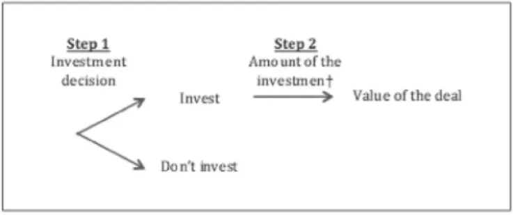
decision should be considered as a two-step process: the first step is a binary decision, either yij,t>0 or yij,t=0.11In the second step, which
occurs once the green light for the investment has been given, the SWF decides the amount to be invested in the specific country.Fig. 1 illus-trates the SWF investment decision-making process that is considered
in a two-tiered model.
Taking into account the rich dynamic structure of the model allows us to test the persistence phenomenon in the investment decision pro-cess, i.e., the fact that SWFs may invest again and for the same amounts in the same target country in the following years once the decision to invest has been taken. The introduction of lagged dependent vari-ables and serially correlated errors in a dynamic panel Tobit model has the effect of making the conventional estimation techniques used in the panel data models inapplicable.Chang (2011b)proposes to esti-mate the dynamic Tobit panel model with the random effects approach. The random effects estimators are obtained by maximizing the corre-sponding likelihood function by specifying the distribution of the error conditional on the regressors. However, the dimension of the integral involved in the calculation of the likelihood function of the dynamic Tobit model, which is as large as the number of censoring periods in the model, makes this likelihood function usually intractable. Taking the initial conditions into account is essential in the dynamic analysis
10An alternative to the two-tiered model is theHeckman (1979)type of
sam-ple selection model. See the discussion inChang (2011b)for the difference between both models.
11We use the average amounts (in USD) of investments in country i from SWFs
in country j in year t as the dependent variable rather than total amounts for two reasons: i) first, certain countries have more than one SWF, and in this case, we take the average amount of investments made in country j by all SWFs in country i for each year; ii) taking the average amounts of investments allow us to control for the number of investments. Making a large number of small investments is different from making only one large investment.
since they are not random, and considering them as exogenous might cause endogeneity problems. To deal with this problem,Chang (2011b)
proposes a maximum simulated likelihood procedure through the corre-lated random effects approach for the two-tiered dynamic Tobit model using the Geweke-Hajivassiliou-Keane (GHK) simulator. In a very recent paper,Xun and Lubrano (2016)show, however, that the use of Heck-man’s initial conditions combined with latent state dependence leads to computational difficulties and an incorrect specification of the true state dependence. Thus, they propose to follow the treatment of initial val-ues proposed byWooldridge (2005). We consider a two-tiered dynamic Tobit panel model initiated byChang (2011a,b)and completed byXun and Lubrano (2016).
We then construct the truncated normal random variables𝜂r ij,t for
censored and uncensored events that can be simulated from, respec-tively,12 𝜂r ij,t= ⎧ ⎪ ⎪ ⎨ ⎪ ⎪ ⎩ Φ−1 ⎛ ⎜ ⎜ ⎝𝜉 r itΦ ⎛ ⎜ ⎜ ⎝ −x′ ij,t𝛽1−yij,t−1𝜆11Iij,t(yij,t−1>0) −𝜆12Iij,t(yij,t−1=0) −c1ij− ∑t−1 k=1Atk𝜂ijr,k Att ⎞ ⎟ ⎟ ⎠ ⎞ ⎟ ⎟ ⎠ yij,t−x′ij,t𝛽2−yij,t−1𝜆21Iij,t(yij,t−1>0) −𝜆22Iij,t(yij,t−1=0) −c2ij− ∑t−1 k=1Atk𝜂rij,k Att (5)
We can then simulate the rthevent probabilities for pair ij at period
t recursively by using the previous periods’ event simulations𝜂r ij,t−kas
given conditional information:
⎧ ⎪ ⎪ ⎪ ⎨ ⎪ ⎪ ⎪ ⎩ Pr(I ij,t=1∣yij,t−1) = Φ ⎛ ⎜ ⎜ ⎝ x′ ij,t𝛽 1+y ij,t−1𝜆11Iij,t(yij,t−1>0) +𝜆12Iij,t(yij,t−1=0) +c1ij+∑tk−=11Atk𝜂ijr,k Att ⎞ ⎟ ⎟ ⎠ fr(yij,t∣yij,t−1) =A1 tt𝜙 ⎛ ⎜ ⎜ ⎝ yij,t−x′ij,t𝛽2−yij,t−1𝜆21Iij,t(yij,t−1>0) −𝜆22Iij,t(yij,t−1=0) −c2ij− ∑t−1 k=1Atk𝜂rij,k Att ⎞ ⎟ ⎟ ⎠ (6)
for occurrence event and amount event probability, respectively. Addi-tionally, we assume that the latent variable y∗ij,tcan be modelled as y∗ij,t=x′ij,t𝛽 +yij,t−1𝜆1Iij,t(yij,t−1>0) +𝜆2Iij,t(yij,t−1=0) +cij+𝜈ij,t (7)
with Iij,tthe indicator function defined as
Iij,t=
{
1 when yij,t>0
0 otherwise
For pair ij, Iij,t=1 if the observed value yij,tis non-zero. In contrast,
Iij,t=0 if yij,tis censored.
In this specification, the two-tiered structure implies that the prob-ability of the investment decision Prob(y∗ij,t)>0 is computed with a first set of parameters(𝛽1, 𝜆1
1, 𝜆 1 2,c
1
ij), while the amount to be invested
(i.e., the conditional expectation of yij,t), given that the investment
decision is determined by a second set of parameters(𝛽2, 𝜆2 1, 𝜆
2 2,c
2
ij).
As already stated, we can observe in this specification that the two-tiered Tobit model allows us to identify in the same model both the
12where r means rthsimulation,𝜂 ∼N(0, 1),𝜉is drawn from uniform (0, 1)
for R times once and fixed during the MLE process,Φand𝜙refer to the CDF and PDF of standard normal density, respectively, A is the lower triangular matrix obtained from the Cholesky decomposition of the compounded errors (individual random effect+AR(1)).
Fig. 1. SWF investment decision-making process.
determinants of the investment decision and the determinants of the amount to be invested, unlike a simple Tobit model. The choice of this model is therefore justified to test forH2. It must be noted that we include the same explanatory variables in each step of the two-tiered model.
Because we have two equations and make a distinction between censored and uncensored events, we have four different values for the𝜆s when using Wooldridge’s specification for the initial values.13 These four parameters indicate the persistence of the investment deci-sion and the amount invested, respectively. Similar to the standard Tobit model, all the other parameters (𝜁, 𝜎u and 𝜎d, which are,
respectively, the error variances of uij,t and dij[an individual random
effect that is unchanged for pair ij across the panel period t] and follow a Normal distribution with zero mean) are common to both steps.14
5. Empirical part
5.1. Description of the macroeconomic variables
The two-tiered dynamic Tobit panel model described above is esti-mated for a large set of explanatory variables that cover the macroe-conomic, geographic, financial, institutional and cultural sectors. The selected macroeconomic variables are the annual GDP growth rate (GDP), the inflation rate (INFLATION) and the real effective exchange rate returns (REER). As a financial variable, we consider the Chinn-Ito index (KAOPEN), which measures the country’s degree of capital account openness. Institutional variables measuring the level of politi-cal risk are corruption (CORRUPTION) and government stability (GOV STAB).15 POLITY is the difference in democracy levels between the SWF country and target country, as defined by the polity IV database. RELIGION is a dummy variable equal to one if the nations have the same major religion, and zero otherwise. DIST is a variable measuring the geographic distance between the acquiring and target country. As inKarolyi and Liao (2017)andKnill et al. (2012), we use for these variables the difference between the SWF and the target nation. Ana-lyzing country-pairs is necessary to calculate the bilateral ”difference” between explanatory variables and the dependent variable. We test whether geographic distance and variables illustrating that economic and institutional distance are determinants of SWF investment
deci-13The interpretations of the true state dependence terms are straightforward:
they control for the previous state’s level of dependency (depending on whether it was an occurred event I( yi,t−1>0) or a null event I( yi,t−1=0), since an
occurred event and a null event have different natures and different recorded scaling) on the current state.
14Other details of the model are given inAppendix 3.
15As GOV STAB represents the government’s ability to carry out its declared
program and its ability to stay in office, this variable is generally lower for democratic countries than for autocratic regimes.
sions, as in a gravity model.16Country-pair variables are computed as17
xij,t=xj,t−xi,t (8)
with j=1,…, 15 the SWFs countries and i=1,…, 72 the target coun-tries.
We then obtain a panel dataset (15,120 observations) that is extremely large compared to those of other studies based on cross-sectional data.18
We also consider control variables representing the SWF charac-teristics such as the size of the fund (LARGE), the origin of the fund (COMMODITY) and the presence of politicians on the board (POLITI-CIANS). LARGE is a dummy variable equal to one if the assets under management of an SWF are greater than USD 100 billion. COMMOD-ITY is a dummy variable equal to one if the funds originate from natural resources, and POLITICIANS is a dummy variable that indi-cates whether politicians are present in the governance of the fund. We expect the variable LARGE to be positively related to SWF invest-ment decisions, particularly to the decision on investinvest-ment amounts. We expect COMMODITY to be positively related to SWF investment decisions abroad because countries with natural resource rent need to deal with commodity prices fluctuations and to prevent Dutch disease. More precisely, a commodity SWF that invests the proceeds from nat-ural resources and fiscal surplus wholly abroad can mitigate the Dutch disease phenomenon and related macroeconomic consequences due to a diversification effect.19We also expect the variable POLITICIANS to be negatively related to investment decisions: SWFs with greater polit-ical involvement tend to support domestic firms rather than invest-ing abroad, as found byBernstein et al. (2013). Appendix 4reports the source and the definition of each variable employed in our study. The correlation matrix has been calculated in order to prevent multi-collinearity problems.20
Table 4reports the summary statistics concerning the variables in the model. First, we can see that the proportion of country-years with SWF investment is 2.1%, which means that 97.9% of the dependent variable observations are equal to zero. The fact that the dependent variable is left-censored at zero with a great number of observations equal to zero justifies the choice of the Tobit model described above. Concerning SWFs characteristics, 96% of SWF countries have at least one SWF managed by politicians, and 86% have at least one large-sized SWF (greater than USD 100 billion). If we look at differences between target and acquiring countries’ characteristics, only 9% of acquiring countries have invested in countries that speak the same language, but 17% invest in countries that share a common religion.21 Concern-ing the geographic distance, only 7% of the investments are made in proximal countries (at a distance of less than 1000 miles), which means that SWFs seem to be indifferent to geographical distance in their investment decision-making process. Finally, we notice that 40% of the investing countries have at least one commodity fund, stress-ing the importance of natural resources in the decision to establish an SWF.
16Gravity models are often used in the international trade literature in order
to analyse the determinants of bilateral trade flows. However, this type of model is not well suited for SWF investment flows, which are frequently equal to zero.
17Country-pair variables measure the geographic, economic and institutional
distance between the SWF country and the host country and have also been tested in terms of their absolute value. The results of the model with the abso-lute value for all these variables are unchanged. To save space, these results are not reported in the paper but are available upon request.
18For example, in their model,Knill et al. (2012)have 3752 observations and
Karolyi and Liao (2017)have 1482 observations.
19SeeCorden and Neary (1982)for more details on this question.
20For the sake of space, we do not report the correlation coefficients, but these
results are available upon request from the authors.
21Because only 9% of acquiring countries invest in target countries that speak
the same language, we do not consider this variable in the model. 7
Table 4
Summary statistics. This table provides the summary statistics for the variables used in our
two-tiered dynamic Tobit model. Details on the variables’ construction are detailed in
Appendix 4.
Mean Median Min Max Std Dev
SWF DUMMY 0.021 0 0 1 0.14 SWF DEAL 1.94 1 1 40 2.74 SWF AMOUNT 499.26 168.25 0.152 9760 1003.86 DIST 6619.64 5414.37 327.46 17,595.10 4191.05 CLOSE 0.07 0 0 1 0.26 GDP 2.69 2.70 −12.82 24.16 5.48 INFLATION −0.007 −0.19 −25.40 12.24 4.98 REER 4.82 1.06 −31.81 217.28 17.66 POLITY −0.54 −0.6 −1 0.8 0.39 KAOPEN 0.12 0 −0.84 1 0.46 RELIGION 0.17 0 0 1 0.38 LANGUAGE 0.09 0 0 1 0.28 GOVSTAB 1.98 2.13 −4.46 5.92 1.87 CORRUPTION −0.23 −0.10 −3.5 3.5 1.64 COMMODITY 0.42 0 0 1 0.49 LARGE 0.86 1 0 1 0.35 POLITICIANS 0.96 1 0 1 0.21 5.2. Results
5.2.1. One-tiered versus two-tiered dynamic Tobit panel models
We test the observation that target country factors do not have the same impacts on the investment decision and the amount to be invested, as indicated inH2. For that, we have estimated both models for com-parison: the one-tiered dynamic Tobit model for panel data and
indi-vidual random effects developed byChang (2011a)described above in Eqs.(1) and (2) and the two-tiered dynamic panel Tobit model initi-ated byChang (2011a,b), and completed byXun and Lubrano (2016)
described in Eqs.(4) and (5). The results of the one-tiered and two-tiered dynamic panel Tobit models with individual random effects are reported inTable 5.
Table 5
One-tiered and two-tiered dynamic Tobit panel results. This table reports results for the one-tiered and
two-tiered dynamic panel Tobit models. Column (2) gives the results of the one-tiered model, columns (3) and (4) report the results for the first equation (decision to invest) and the second equation (amount to be invested) of the two-tiered model, respectively. The summary statistics of these variables are presented in
Table 4.Appendix 4presents details on the variable construction.
One-tier Two-tier Eq.(1) Eq.(2) CONSTANT −112.600∗∗∗ [20.330] −5.6680∗∗∗ [0.4553] 14.749∗∗∗ [0.711] INFLATION 1.0870∗∗ [0.3593] 0.0023 [0.0079] −0.0013 [0.0237] REER −0.1304 [0.0705] 0.0026 [0.0019] 0.0166∗∗ [0.0063] POLITY −11.6000 [6.349] −0.8367∗∗∗ [0.2465] −1.6312∗∗∗ [0.4714] KAOPEN 14.8500∗ [7.252] 0.3040 [0.1879] −0.9840∗∗∗ [0.3402] GOVSTAB 1.6390 [0.8935] 1.1410∗∗∗ [0.0353] 0.0520 [0.0740] POLITICIANS 15.1500∗ [7.0250] 0.3371∗ [0.1436] −0.0768 [0.2713] DIST −0.0011∗ [0.0005] −0.0001 [0.0001] −0.0001 [0.0001] GDP 0.0230 [0.2170] −0.0001 [0.0065] −0.0089 [0.0211] CORRUPTION −1.7880 [1.6400] 0.0066 [0.0536] −0.0060 [0.1069] RELIGION −1.0280 [1.3340] −0.2148 [0.2004] −0.1517 [0.3693] LARGE 30.0000∗∗∗ [8.0330] 0.0491 [0.1044] −0.2088 [0.1987] COMMODITY −28.130∗∗ [9.1100] −0.1817 [0.1193] −0.1479 [0.2238] 𝜆1 −37.9600 [34.5900] 0.1108∗∗∗ [0.0150] 0.0843∗∗ [0.0263] 𝜆2 7.3310 [5.8070] 0.3811 [0.2416] 1.4477∗∗ [0.4956] Log-likelihood −2331.121 −1790.16 BIC 4835.47 3897.905
Several elements illustrate the performance of the two-tiered dynamic Tobit panel model compared to the one-tiered model. First, the log-likelihood function has a much higher value than that of the corresponding one-tiered model and the BIC value is smaller in the two-tiered.22 Second, this model relaxes many constraints that allow the asymmetric effects between the two equations to be captured. In particular, variables capturing the political distance between both tries, such as POLITY, GOV STAB and the variable measuring the coun-try’s degree of capital account (KAOPEN), are significant in the two-tiered model but not in the one-two-tiered model. Finally, the individual effect parameters (𝜆′s) are significant in the two-tiered model but not in the one-tiered model, which means that the dynamic component of the model is significantly different from zero only when we consider the two-tiered model. This finding suggests that ignoring the two-stage nature of the investment decision and assuming that the country factors have the same impact in both stages as in a one-tiered Tobit model is therefore a restrictive approach and leads to biased conclusions, which confirms H2. Our result also confirms the significance of the lagged
dependent variable in the two-tiered panel model compared to the one-tiered panel model, meaning that the dynamic component is crucial in the SWF’s investment decision process and should be taken into account in the two-tiered model.
5.2.2. Results of the two-tiered dynamic Tobit panel model
Results of the two-tiered dynamic Tobit model with panel data are given in Table 6. Panel A displays the results of the first stage (invest-ment decision), and Panel B shows the results of the second stage (the decision about the amount to invest). The same explanatory variables have been included in each step of the two-tiered model. For both equa-tions, we include in the first column all the possible explanatory vari-ables, corresponding to the full model. We then report the estimates of different restricted versions of this model with variables estimated one by one (columns (2) to (6)). Column (7) gives the results of the most parsimonious model.
First, we find that most country-pair variables are significant in both Panel A and in Panel B, which means that country factors (macroeco-nomic, geographical, institutional and cultural factors) turn out to be key determinants of SWFs’ investments. This result is also in line with the conclusions of some recent studies, according to which SWFs’ moti-vations may be non-financial (Chhaochharia and Laeven (2009), Bern-stein et al. (2013) or Knill et al. (2012)). The importance of country factors also constitutes a key point in order to evaluate the role of SWF investments in crisis periods. If they were exclusively driven by the quest for financial returns, they could be a destabilizing force for finan-cial markets. In contrast, we show that macroeconomic determinants are crucial for SWFs. This finding tends to support the idea that SWF investments follow long-run horizon strategies, constituting potential market stabilizers in periods of turmoil.
Second, our estimation results indicate the following. i) Country-level factors have a positive impact not only on the investment decision but also on the choice of the amount to be invested, which is conditional on the investment decision. This situation is clearly the case for the vari-able POLITY, which is significant in both equations. ii) These country factors driving the SWF investment decision are not the same as those used to set the amount to be invested, consistent with H2. More pre-cisely, we find that the financial openness index KAOPEN does not mat-ter for the decision to invest, whereas a high difference in the financial openness index between the SWF and target country tends to decrease the average value of the deal. In contrast, a higher government stability
22 In the one-tiered model, we have 15 parameters for 𝛽and 𝜆and three other
parameters in the error component (totally 18 parameters), while in the two-tiered model, we have double the number of parameters for 𝛽and𝜆, but the two tiers share the same set of error components as in the one-tiered model (a total of 33 parameters).
difference (GOVSTAB) increases the probability of an SWF investment but does not affect the amount to be invested. In support of this result,
Knill et al. (2012)) find that bilateral political relations between SWF and target countries are an important determinant of why SWFs invest in a given country, but they matter less in determining how much to invest. In light of our results, we can conclude that SWFs’ investment decisions are the outcome of a complex process. It is therefore essen-tial to distinguish the factors that influence the decision to invest from those that determine the amount of the investment.
RegardingH1, which stresses that SWFs tend to invest in countries that share similar macroeconomic, geographical and institutional char-acteristics, we find some contrasting results on macroeconomic and cul-tural factors. While the variable GDP is never significant, we observe that the coefficient for REER is significantly positive in Panel B but not in Panel A, whereas it is the reverse for the variable INFLATION. This finding suggests that as the difference in terms of REER increases, the tendency for an SWF to invest large amounts increases. In contrast, as the difference in terms of inflation increases, an SWF becomes more likely to invest. These results can be interpreted to mean that SWFs may prefer to invest in countries that do not share the same macroeconomic characteristics as the home country. As seen in the previous section, the majority of the most active SWFs are located in Asia and the Mid-dle East and show a clear preference to invest in developed countries (North America and West Europe) that have a more stable economy in terms of both inflation and exchange rates.
Concerning cultural factors, unlikeChhaochharia and Laeven (2009)
andBernstein et al. (2013), we do not find empirical support that SWFs are focused on countries that share a similar culture or are geograph-ically close (the variables RELIGION and DIST are not significant in Panel A or in Panel B). This result does not corroborate the idea that SWFs invest while keeping in mind religious or cultural proselytism (Islamic finance). In the same way, we do not find evidence of a home or a region bias in SWFs’ investment policies.
However,H1is well supported by our results on political and insti-tutional factors. The significance of POLITY, GOV STAB, KAOPEN and POLITICIANS clearly reveal that country factors are essential to SWFs’ investment decision process. More specifically, we find that POLITY and KAOPEN are negatively related to SWF investments (the invest-ment decision and/or the amount to be invested), meaning that SWFs are more likely to invest in countries with which they have lesser dif-ferences in their levels of democracy and financial openness. The first result, which is consistent withKarolyi and Liao (2017), means that SWFs prefer to invest in countries that have a similar level of democ-racy as the home country.23Moreover, the variable GOV STAB is pos-itively related to SWFs’ investment decisions but does not impact the amounts to be invested, which means that an SWF is more likely to invest in a country when government stability is different. Contrary to
Bernstein et al. (2013), we find that the presence of politicians in the fund significantly influences the decision to invest abroad. Finally, the characteristics of the fund itself, such as its size or its origin (whether a commodity fund or not), do not seem to influence its investment strat-egy.
H3deals with the autoregressive terms and assumes that when an SWF invests in a country, it is likely to invest in that country again in the future. In other words, the true state dependence coefficients (𝜆′s) would be significantly different from 0. It appears that indeed, in Panel A, only𝜆1 is significant, which indicates that an SWF thus
tends to reinvest in a country in which it has already invested. We also observe that𝜆2 is not significantly different from 0, which indicates
that there is no investment barrier for countries in which SWFs have never invested. For Panel B, both𝜆1and𝜆2are significant, supporting
the idea of inertia in the amount invested by SWFs.
23However,Knill et al. (2012)) find that POLITY is positively related to SWF
investment (the investment decision and the amount to be invested). 9
Table 6
Two-Tiered Dynamic Tobit Panel Results. This table reports results for the panel analysis of investment decisions (Panel A: first equation of the two-tiered
Tobit model) and the average amount invested by SWFs (Panel B: second equation of the two-tiered Tobit. Column (1) gives the results for the full model, columns (2) to (6) report the estimates of different restricted versions of this model with variables estimated one by one. Column (7) gives the results of the parsimonious model. The summary statistics of these variables are presented inTable 4.Appendix 4presents details on the variables’ construction.
(1) (2) (3) (4) (5) (6) (7)
Panel A: decision to invest (first equation) CONSTANT −5.668∗∗∗ [0.455] −5.335∗∗∗ [0.3772] −5.401∗∗∗ [0.355] −5.807∗∗∗ [0.334] −5.892∗∗∗ [0.408] −5.862∗∗∗ [0.433] −5.797∗∗∗ [0.459] INFLATION 0.002 [0.008] 0.024∗∗ [0,008] 0.025 [0.112] REER 0.003 [0.002] 0.002 [0.002] 0.002 [0.003] POLITY −0.837∗∗∗ [0.247] −1.136∗∗∗ [0.174] −0.816∗∗ [0.257] KAOPEN 0.304 [0.188] −0.040 [0.181] 0.245 [0.157] GOV STAB 0.141∗∗∗ [0.035] 0.208∗∗∗ [0.033] 0.128∗∗∗ [0.037] POLITICIANS 0.337∗ [0.144] 0.232 [0.138] DIST −0.000 [0.000] GDP −0.000 [0.007] CORRUPTION 0.007 [0.054] RELIGION −0.215 [0.200] LARGE 0.049 [0.104] COMMODITY −0.182 [0.119] 𝜆1 0.111∗∗∗ [0.015] 0.132∗∗∗ [0.016] 0.137∗∗∗ [0.015] 0.133∗∗∗ [0.015] 0.394∗∗∗ [0.062] 0.382∗∗∗ [0.049] 0.114∗∗∗ [0.021] 𝜆2 0.381 [0.242] 0.480∗ [0,235] 0.545∗ [0.233] 0.524∗ [0.233] 0.420 [0.284] 0.193 [0.212] 0.440 [0.332] Panel B: Amounts to be invested (second equation)
CONSTANT 14.749∗∗∗ [0.711] 14.44∗∗∗ [0.529] 14.327∗∗∗ [0.521] 13.514∗∗∗ [0.483] −0.200 [0.288] −0.598 [0.568] 14.260∗∗∗ [0.684] INFLATION −0.001 [0.024] 0.046∗ [0.021] 0.011 [0.019] REER 0.017∗∗ [0.006] 0.018∗∗ [0.061] 0.015∗ [0.007] POLITY −1.631∗∗∗ [0.471] −2.022∗∗∗ [0.293] −1.566∗∗∗ [0.397] KAOPEN −0.984∗∗ [0.340] −1.582∗∗∗ [0.320] −1.081∗∗∗ [0.319] GOV STAB 0.052 [0.074] 0.180∗∗ [0.055] 0.041 [0.068] POLITICIANS −0.077 [0.271] 0.0212 [0.260] DIST −0.000 [0.000] GDP −0.009 [0.021] CORRUPTION −0.006 [0.107] RELIGION −0.151 [0.369] LARGE −0.209 [0.199] COMMODITY −0.148 [0.224] 𝜆1 0.084∗∗ [0.026] 0.114∗∗∗ [0.025] 0.118 [0.024] 0.110∗∗∗ [0.024] 0.454∗∗∗ [0.053] 0.490∗∗∗ [0.076] 0.084∗ [0.038] 𝜆2 1.448∗∗ [0.496] 2.014∗∗∗ [0.455] 2.051∗∗∗ [0.446] 1.912∗∗∗ [0.441] 1.983∗∗∗ [0.313] 2.238∗∗∗ [0.414] 1.446∗ [0.639] 𝜎u 1.503∗∗∗ [0.056] 1.584∗∗∗ [0.064] 1.568∗∗∗ [0.056] 1.548∗∗∗ [0.068] 1.511∗∗∗ [0.052] 1.565∗∗∗ [0.067] 1.486∗∗∗ [0.052] 𝜎d 1.598∗∗∗ [0.161] 1.632∗∗∗ [0.173] 1.624∗∗∗ [0.169] 1.619∗∗∗ [0.100] 2.138∗∗∗ [0.127] 1.967∗∗∗ [0.219] 1.578∗∗∗ [0.161] 𝜁 −0.321∗∗∗ [0.054] −0.339∗∗∗ [0.056] −0.274∗∗∗ [0.053] −0.310∗∗∗ [0.056] −0.360∗∗∗ [0.041] −0.376∗∗∗ [0.046] −0.319∗∗∗ [0.050] Log-Likelihood −1790.16 −2040.09 −2042.39 −2012.29 −1990.08 −1975.75 −1911.33 BIC 3897.905 4186.042 4190.642 4130.442 4086.022 4057.362 4024.759 Iterations 697 472 522 476 388 406 532
Table 7
Two-tiered dynamic Tobit panel results – Robustness checks. This table reports results for
the panel analysis of the decision to invest and the average amount invested by SWFs, taking into account the sign of the difference. The explanatory variables (x) have been calculated with the following formula: xij=xj−xi, where i is the target country and j is the acquirer country. We then
decided to reestimate the model by taking into account both the cases in which xj>xi(xij+) and
xj<xi(xij-). Column (1) gives the results for Panel A (decision to invest), and column (2) gives
the results for Panel B (amounts to be invested).
Panel A Panel B CONSTANT −4.757∗∗∗ [0.421] 14.440∗∗∗ [0.529] INFLATION+ 0.026 [0.019] −0.025 [0.035] INFLATION- 0.050∗∗ [0.018] 0.019 [0.038] REER+ 0.012 [0.008] 0.033 [0.023] REER- −0.005 [0.004] −0.002 [0.009] POLITY+ −0.758 [0.600] −1.503 [1.160] POLITY- −0.344 [0.375] −1.361∗∗ [0.473] KAOPEN+ −0.026 [0.339] −1.637∗∗∗ [0.453] KAOPEN- 1.091∗∗∗ [0.307] 0.116 [0.509] GOV STAB+ 0.177∗∗∗ [0.039] 0.080 [0.074] GOV STAB- 0.052 [0.097] −0.337 [0.201] 𝜆1 0.084∗∗ [0.074] 0.081∗∗ [0.025] 𝜆2 0.208∗∗∗ [0.235] 1.433∗∗ [0.447] 𝜎u 1.470∗∗∗[0.049] 𝜎d 1.498∗∗∗[0.127] 𝜂 −0.191∗∗∗[0.056] Log-Likelihood −1833.78 Iterations 538
∗ Significant at 5%; ∗∗ significant at 1%; ∗∗∗ significant at 0.1%. Standard errors are in brackets. Finally, our error component assumption with consideration of a
random effect+AR(1) process allows us to capture the spurious state dependence parameter𝜁(auto-correlation of errors) in a very consistent and significant way across different specifications. Thus, we managed to avoid the unexpected estimation confusion in identifying the true state dependence features.
5.3. Refinement of country-pair variables
The results found inTable 5allow us to determine if country-pair variables are significant but not to determine the sense of the differ-ence: does the probability of investment made by the SWF country (the investment decision and/or the amount to be invested) tend to increase or decrease when the difference between SWF country factors and those of target country is negative (positive)? To answer this question, the country-pair variables described in Eq.(7)were split, allowing us to determine if there is a difference in favor of the acquirer or of the host country:
xij,t,+=xj,t−xi,t with xj>xi (9)
xij,t,−=xj,t−xi,t with xj<xi (10)
The results are displayed inTable 7. Panel A displays the results of the first stage (investment decision) and Panel B the results of the sec-ond stage (the decision about the amount to invest). These new results confirm the role of political and institutional variables in the attraction of SWFs: stability of the government, democracy index and degree of
capital account openness. In particular, we find that political stability of the target country is a factor that contributing to the attractiveness when acquirer country is less stable politically (GOV STAB+is positive and highly significant in Panel A).
Once again, we find that the determinants driving the SWF invest-ment decision are not the same as those used to set the amount to be invested. More precisely, POLITY- and KAOPEN+ are negative and sig-nificant in panel B, which means that SWFs are more prone to investing large amounts in countries that are less democratic and more financially open. Strikingly, KAOPEN- is significantly positive in panel A, whereas KAOPEN+ is significantly negative in panel B. This result means that the target country’s degree of financial openness matters for both the SWFs’ investment decision and the amount to be invested.
6. Conclusion
One of the main concerns about SWFs’ investment strategy, which has been widely studied in the literature, is that SWFs could invest for non-financial reasons. This paper aims to shed light on the question of the motivation of SWFs in their investment decision and, more pre-cisely, whether country-level factors such as macroeconomic, political, institutional or cultural factors can explain this decision. More specif-ically, we develop an approach that takes into account the fact that the cross-border investment decision for an SWF is the outcome of a complex decision-making process. To do so, we estimate a two-tiered dynamic Tobit panel model recently developed byChang (2011b)and extended byXun and Lubrano (2016), which allows us to test three important aspects of this decision-making process: i) the independence 11
amounts invested.
The results of the model also suggest that country-level factors can affect SWFs’ investment decision, which means that financial motives are not the exclusive target of their investment strategy. In particular, we find that SWF investments are driven by macroeconomic, political and institutional considerations. The findings regarding macroeconomic variables show that more mature economies tend to attract SWF invest-ments. Our findings also show that SWFs that involve politicians have a much greater likelihood of investing abroad and tend to be attracted to countries with greater political stability. Finally, we find that SWFs are more prone to investing large amounts in countries that are less demo-cratic and more financially open, which means that the determinants driving the investment decision are not the same as those used to set the amount to be invested. Taken as a whole, our results lend support to the idea that SWFs are safe in the choice of target countries concerning their investment decisions but behave as more opportunistic investors concerning the amount to be invested. Our results shed new light on SWFs’ investment strategy for regulators seeking to enhance financial stability, thereby motivating – in line with the Santiago principles – a better evaluation of macroeconomic risks.
of the SWF decision regarding where and how much to invest (which justifies the choice of the two-tiered model); ii) the persistence phe-nomenon in the investment decision, which is accounted for in the dynamic dimension of the model; iii) the inclusion of the temporal dimension and the unobserved heterogeneity in the dependent variable considered in the panel dimension of the model.
Several insights emerge from our analysis. From an econometric per-spective, the key insight from this paper is that the choice of the model allows us to independently estimate the decision of where and how much to invest. The results of the analysis indicate that the determi-nants driving the SWF investment decision are not the same as those used to fix the amount to be invested. This finding suggests that ignor-ing the two-stage nature of the investment decision and assumignor-ing that the country factors have the same impact in both stages as in a Tobit model is a restrictive approach. On the basis of our results, we can con-clude that country-level factors are key determinants not only of the investment decision but also of the choice of the amount to be invested. In the same spirit, we find that the dynamic component of the two-tiered panel model is crucial, suggesting that SWFs have a tendency to invest in the target country in the years after the decision to invest has been taken and to do so in a persistent, dynamic manner in terms of the
Appendices
Appendix 1. Characteristics of SWFs
Country Fund name Assets Under
Management
Founding date
Source of the funds
Policy purpose Presence of politicians on the SWF board
Australia Queensland Investment Corporation 70.6 1992 Fiscal Unknown Yes
Australia Victorian Funds Management Corpo-ration
46.6 1994 Unknown Unknown No
Australia Australian Future Fund 95 2006 Non-commodity Saving No
Bahrain Bahrain Mumtalakat Holding Com-pany
10.5 2006 Non-commodity Saving Reserve investment Unknown
China China Investment Corporation 652.7 2007 Non-commodity Reserve investment Yes
China China SAFE Investment 567.9 1997 Non-commodity Reserve investment Yes
China National Social Security Fund 201.6 2000 Non-commodity Reserve investment Yes
China China-Africa Development Fund 5 2007 Non-commodity Reserve investment Yes
France France Strategic investment fund 25.5 2008 Non-commodity Pension reserve Yes
Kazakhstan Samruk Kazyna National Wealth Fund 77.5 2008 Non-commodity Stabilization Saving Pension reserve
No
Kuwait Kuwait Investment Authority 548 1953 Oil and gas Stabilization Saving Yes
Libya Libyan Investment Authority 66 2006 Oil and gas Saving Yes
Malaysia Khazanah Nasional 40.5 1993 Non-commodity Saving No
New Zealand
New Zealand Superannuation Fund 28.98 2001 Non-commodity Pension reserve Yes
Oman State General Reserve Fund 13 1980 Oil and gas Stabilization Reserve
invest-ment
No
Oman Oman Investment Fund 6 2006 Oil and gas Reserve investment No
Qatar Qatar Investment Authority 170 2005 Oil and gas Saving Reserve investment No
Saudi Ara-bia
Kingdom Holding 19.6 1996 Oil and gas Reserve investment Unknown
Singapore Government of Singapore Investment Corporation
320 1981 Non-commodity Saving Reserve investment No
Singapore Temasek 177 1974 Non-commodity Saving Reserve investment No
South Korea Korea Investment Corporation 72 2005 Non-commodity Reserve investment Yes
UAE Dubai Holding NA 2004 Oil and gas Unknown Yes
UAE Dubai World NA 2004 Oil and gas Reserve investment Yes
UAE Abu Dhabi Mubadala Development Company
60.9 2002 Oil and gas Reserve investment No
UAE Abu Dhabi International Petroleum Investment Company
68.4 1984 Oil and gas Reserve investment Yes
UAE Abu Dhabi Investment Authority 773 1976 Oil and gas Saving Reserve investment Yes
UAE Ras-al-Khaimah Investment Authority 1.2 2005 Oil and gas Reserve investment No
UAE Investment Corporation of Dubai 70 2006 Oil and gas Reserve investment No