HAL Id: hal-01096110
https://hal.inria.fr/hal-01096110
Submitted on 16 Dec 2014
HAL is a multi-disciplinary open access
archive for the deposit and dissemination of
sci-entific research documents, whether they are
pub-lished or not. The documents may come from
teaching and research institutions in France or
abroad, or from public or private research centers.
L’archive ouverte pluridisciplinaire HAL, est
destinée au dépôt et à la diffusion de documents
scientifiques de niveau recherche, publiés ou non,
émanant des établissements d’enseignement et de
recherche français ou étrangers, des laboratoires
publics ou privés.
On Program Equivalence with Reductions
Guillaume Iooss, Christophe Alias, Sanjay Rajopadhye
To cite this version:
Guillaume Iooss, Christophe Alias, Sanjay Rajopadhye. On Program Equivalence with Reductions.
21st International Static Analysis Symposium (SAS’14), Sep 2014, Munich, Germany. �hal-01096110�
On Program Equivalence with Reductions
Guillaume Iooss1,2, Christophe Alias2, Sanjay Rajopadhye1 1 Colorado State University
2 ENS-Lyon, CNRS UMR 5668, INRIA, UCB-Lyon
Abstract. Program equivalence is a well-known problem with a wide range of applications, such as algorithm recognition, program verification and program op-timization. This problem is also known to be undecidable if the class of programs is rich enough, in which case semi-algorithms are commonly used. We focus on programs represented as Systems of Affine Recurrence Equations (SARE), defined over parametric polyhedral domains, a well known formalism for the
polyhedral model. SAREs include as a proper subset, the class of affine con-trol loop programs. Several program equivalence semi-algorithms were already proposed for this class. Some take into account algebraic properties such as asso-ciativity and commutativity. To the best of our knowledge, none of them manage reductions, i.e., accumulations of a parametric number of sub-expressions using an associative and commutative operator. Our main contribution is a new semi-algorithm to manage reductions. In particular, we outline the ties between this problem and the perfect matching problem in a parametric bipartite graph.
1
Introduction
Program equivalence is an old and well-known problem in computer science with many applications, such as program comprehension, algorithm recognition [1], program ver-ification [2,3], semi-automated debugging, compiler verver-ification [4], translation valida-tion [5,6,7,8] to name just a few. However, the program equivalence problem is known to be undecidable as soon as the considered program class is rich enough to be interest-ing. Moreover, if we account for the semantic properties of objects manipulated in the program and relax the considered equivalence, the problem becomes harder.
Considerable prior work on program equivalence exists, in particular in the context of translation validation (in which we seek to prove the equivalence between a source and a target program). Necula [5] builds a correlation relation between the control flow graphs of the source and the target programs, and relies on a solver to check whether this relation is a bisimulation [9,10]. Such an approach is restricted to structure
preserv-ingoptimizations, and cannot deal with advanced transformations like loop reordering which can arbitrarily change the control structure of the program. Zuck et al. [7] over-ride these limits and introduce “permutation rules” to validate a reordering transforma-tion. They also derive a runtime test for advanced loop optimizations. When a problem is detected, the code escapes to an unoptimized version. Kundu et al. [8] combine the benefits of these approaches to check statically that an optimizing transformation is sound.
In this paper, we focus on Systems of Affine Recurrence Equations (SARE) with re-ductions. SAREs are a formalism for reasoning about many compute- and data-intensive
programs in the polyhedral model and used for in automatic parallelization. A
reduc-tion is the application of an associative and commutative operator to a set of (sub) expressions.3Thus, in order to decide equivalence between two reductions, we need to
take care of the associativity and commutativity properties over a potentially parametric number of elements.
A well known semi-algorithm for SAREs was proposed by Barthou et al [11]. The idea is to encode the problem of equivalence of two programs into a Memory State
Au-tomaton, i.e., an automaton whose states are associated with vectors and whose edges are associated with conditions on these vectors. The equivalence problem on SARE can be reduced to a reachability problem on this automaton, which is also undecidable, but on which several heuristics are applicable (based on the transitive closure operation). However, no semantic properties are considered (the equivalence is purely structural). Shashidhar et al. [12] proposed another equivalence algorithm based on Array Data
Dependence Graph(ADDG). Their algorithm manages associativity and commutativ-ity over a finite number of elements. However, because complicated recurrences are managed by unfolding loops, it cannot manage parametrized programs. Verdoolaege et al [13] proposed an improved formalism based on a dependence graph, which allows them to manage parametrized program. They also present an alternative way to deal with recurrences, based on the widening operation. In the two previous papers, com-mutativity is managed by testing every permutation of the arguments of operators until we find a good one. This approach is no longer possible if the number of arguments is parametrized. Karfa et al. [14] also proposed an algorithm to decide equivalence based on ADDG. The idea behind their equivalence checking is to build an arithmetic expres-sion corresponding to the computation done by the considered program. By normaliz-ing this expression, they are able to manage the semantic properties of binary operators. However, because they need to have a finite arithmetic expression, they are not able to manage recursion and reductions.
In this paper, we propose a semi-algorithm which decides the equivalence of two programs containing reductions. More precisely, our contributions are as follows.
– Building on the Barthou et al. formalization, we propose a rule to manage the equivalence between two reductions (Section 3). This rule can be extended to cover equivalence with a finite number of reductions combined with the same operator. – The previous rule maps corresponding sub-terms of both reductions through a
bi-jection. We propose a semi-algorithm to infer such bijection (Section 4) that • first extracts the set of constraints our bijection needs to satisfy,
• transforms them into a finite list of partial bijection (i.e., bijections defined over subsets of the actual space), and finally
• simply combines these partial bijections together to form our bijection. We show the relation between our problem of partial bijection combination, and the perfect matching problem on a parametric bipartite graph.
– We propose heuristics to solve the perfect matching problem for graphs of para-metric size. One in particular, is based on a novel extension of the well known
augmenting pathalgorithm (that addresses only the non-parametric case).
3Some authors do not require commutativity, in which case a reduction must be applied to an
orderedset of sub-expressions. In this paper we would like to allow many general reordering transformations, and therefore insist on commutativity.
2
Preliminaries
We first describe the class of programs we consider. We define the notion of equivalence modulo associativity and commutativity and detail Barthou’s semi-algorithm, since it serves as our starting point.
2.1 System of Affine Recurrence Equations with reductions
A reduction is the application of an associative and commutative binary operator ⊕ on a parametric set of (sub) expressions. For example L
0≤i<N
A[i] is a reduction of N sub-expressions A[i], N being a parameter. We study the equivalence between programs represented as Systems of Affine Recurrence Equations (SARE) with reductions, defined as follows
Definition 2.1. A SARE with reductions is a set of equations of the form:
X[i] = .. .
E xpr(. . . Y[uY,k(i)] . . .), if i ∈ DX1 ..
.
where X is defined over DX=U k
DX k ⊆ Z
d, the DX
k being disjoint.
– X, Y, . . . are called variables. They are defined over a polyhedral domain DX and
associate a value to each point of their domain.
– Some variables are marked as input (or output) variables. An input variable cannot
be defined by an equation of the SARE and any other variable X has exactly one equation which computes its value, for each point of DX.
– E xpr[i] is an expression and may be one of
• A variable Y[uY,k(i)] where uY,kis an affine function.
• An operation f (E xpr1[i], . . . E xprn[i]) where f is a n-ary operator. • A reduction L
π(i′)=i
E xpr′[i′] where π is called the projection function. Because
i′∈ D
E xpr′, we can control the set of expressions summed together through the
definition domain of Expr′.
Example 2.1. The standard matrix multiplication algorithm for N × N matrices is de-scribed by following SARE with inputs A and B, and output C, each defined over DA =DB =DC=[|0; N − 1|]2. C[i,j] = N−1 P k=0 A[i,k] * B[k,j]
Our equivalence semi-algorithm accepts as inputs, a pair of SAREs with reductions. We currently do not treat “recursive” reductions, i.e., those in which a variable being defined by a reduction appears inside the reduction loop, i.e. we must not encounter a parametric number recursions in the computation flow while computing an output
value. For example, the following SARE, that combines a parametric number of terms of the variable A to define the ithe element of A, is not accepted:
O = A[N] A[i] = P 0≤k<i A[k] if 0 < i ≤ N 1 if i=0
2.2 Equivalence modulo associativity and commutativity
There are several notions of equivalence between programs. The simplest one is called
Herbrand equivalenceand corresponds to the structural equivalence (the computation performed by both programs is identical). We also need to give a mapping between the
inputsof the two programs, to say which inputs are equivalent. For example, the SARE O[i] = f(A[i]) + B[i]is equivalent to the SARE O′[i] = Temp′[i] + B′[i],
Temp′[i] = f(A′[i])assuming that the input pairs A/A′ and B/B′ are equivalent. It
will be also equivalent to any SARE obtained by applying any data-dependence pre-serving transformation (i.e. a transformation which does not modify the computation). However, if we permute the arguments of the addition (commutativity) in one of them, it will no longer be equivalent to the other. The problem of Herbrand equivalence between general SAREs is undecidable [11].
We consider Herbrand equivalence modulo associativity and commutativity: a SARE is equivalent to any other SARE obtained by applying any data-dependence preserving transformation plus associativity and commutativity of the corresponding binary oper-ators. For example, the SARE O[i] = (A[i] + 2) + B[i] is equivalent to O′[i]
= Temp′[i] + 2, Temp′[i] = A′[i] + B′[i]. Moreover, because reduction
implic-itly uses associativity and commutativity, we need this extended notion of equivalence to compare SAREs with reductions. For example, under such equivalence, the SARE O[i] = P
i
A[i]is equivalent to O′[i′] = P i′
A′[N-i′]
2.3 Deciding Herbrand equivalence of two SAREs
Barthou et al. [11] proposed a semi-algorithm to decide Herbrand equivalence of SAREs. It first builds an equivalence memory state automaton encodeing the equivalence prob-lem and then studies the accessibility set of particular states of this automaton. Definition 2.2. A Memory State Automaton (MSA) [11] is a finite automaton where:
– Every state p is associated with an integer vector vpof some dimension np. – Every transition from p to q is associated with a firing relation Fp,q∈ Znp× Znq. – A transition from hp, vpi to hq, vqi can only happen if (vp, vq) ∈ Fp,q.
We say that a state p is accessible iff there exists a finite path from the initial state
p0to p for some associated vector. The accessibility relation of a state p is:
Step 1: Building the equivalence MSA: Consider two SAREs. We use the convention that expressions, operators and indices of the second SARE are “primed” (e.g., X′, E′
1,
. . . ). The equivalence MSA is defined (and built) in the following way:
– States: A state is labeled by an equation e(i) = e′(i′) and is associated with the
vector (i, i′).
– Initial state: The initial state of the automaton is O[i0] = O′[i′ 0]
– Final state: There are two kinds of final states: the success states and the failure
states. The failure states are:
• f (. . .) = f′(. . .) where f and f′are different operators,
• Ik[i] = f′(. . .) or f (. . .) = Ik′[i ′],
• Ik[i] = I′k′[i] where Ikand Ik′′are not corresponding inputs. In contrast, the accept states are:
• f () = f′() (i.e., two identical constants)
• Ik= Ik′′where Ikand Ik′′are corresponding inputs.
– Transitions: We have 3 types of transitions (rules) in the equivalence MSA:
De-compose, Compute and Generalize, as described in Fig 1. The Decompose rule deals with operators and simply says that two expressions using the same operator are equivalent iff their arguments are equivalent. The Compute rule allows us to “unroll” a definition and creates a state per case. Note that for each value (i, i′)
as-sociated with the source state, there is only one accessible state among the created states. The Generalize rule is useful to deal with recursions. It replaces an affine expression by a fresh index, allowing us to go into a state we may have already encountered, but with different index values.
f(E1(i), . . . , En(i)) = f (E1′(i′), . . . , E ′ n(i′)) E1(i) = E1′(i′) . . . En(i) = E′n(i′) Decompose rule X[i] = . . . E xpr1(i) = . . . E xprk(i) = . . . i ∈ ∆1 i ∈ ∆k . . . where X[i] = i ∈ ∆1: E xpr1(i) . . . : . . . i ∈ ∆k: E xprk(i) Compute rule . . .X[u(i)] . . . = . . . . . .X[ j] . . . = . . . j = u(i)
where j is a fresh variable.
Generalize rule
Fig. 1. Construction rules for the equivalence automaton
Step 2: Equivalence and reachability problem in the equivalence automaton: Intu-itively, if a state E xpr[i] = E xpr[i′] can be reached for a given (i, i′), then these two
expressions must be equivalent so that the two SAREs are equivalent. Thus, the equiv-alence problem between the two considered SAREs can be decided by studying the accessibility sets of the success and failure states.
Theorem 2.1 (from [11]). Two SAREs are equivalent iff, in their equivalence MSA: – All failure states are not accessible from the start state.
– The accessibility relation of each success state is included in the identity relation.
Indeed, a failure state corresponds to the comparison of two expressions which are obviously not equivalent. The condition of the success states that, if we start from the initial states with an equality of the indices of the outputs, the indices of any reachable success state must be the same (i.e., I[i] cannot be identical to I[j] for i , j).
Example: As an example, let us compare the following SARE with itself:
O = A[N]
A[i] =( 1 ≤ i ≤ N : f (I[i], A[i − 1])
i =0 : I[0]
where O is the output of the SARE and I the input. The equivalence automaton is the following (success states are in blue and failure states in red):
O = O′ A[N] = A′[N] A[i] = A′[i′] I[0] = A′[i′] f(I[i], A[i − 1]) = A′[i′] I[0] = I′[0] I[0] = f (I′[i′], A′[i′− 1])
f(I[i], A[i − 1]) = I′[0] f(I[i], A[i − 1]) = f (I′[i′], A′[i′− 1])
I[i] = I′[i′] A[i − 1] = A′[i′− 1] (Comp) (Gen) i = N, i′= N (Comp) i =0 i >0 (Comp) i′=0 i′>0 i′=0 (Comp) i′ >0 (Dec) (Gen) i = i −1 i′= i′− 1
Notice how the automaton has a cycle: it corresponds to the comparison between the recursions of both SARE. We can notice that, for every state of the automaton, we have i = i′(indeed, for each transition we are modifying i, we are also modifying i′in
the same way). Thus, because the reachability set of the failure states are respectively {i, i′| i = 0 ∧ i′>0} and {i, i′| i > 0 ∧ i′=0}, then they are both empty. Moreover, the
equalities that needs to be satisfied when reaching a success state are respectively 0 = 0 (trivially satisfied) and i = i′(satisfied). Thus, according to Thm 2.1 these two SARE are equivalent.
Limitation of the equivalence algorithm: This algorithm only checks Herbrand equiv-alence, semantic properties like associativity/commutativity of operators are not taken into account. For instance, if we try to compare the SAREs O = I1+ I2and O′= I2′+ I
′ 1,
the equivalent automaton will have a decompose rule which will generate two failure states of labels (I1= I2′) and (I2= I1′).
3
Decompose Reduce rule
In the previous section, we presented Barthou’s equivalence algorithm, based on the construction of an equivalence automaton. This algorithm can be extended to manage reductions, by adding a new construction rule (called Decompose Reduce):
L π(k)=i E[k] = L π′(k′)=i′ E′[k′] E[k] = E′[k′] σ(k) = k′
The idea of this rule is to map every occurrence of the left reduction E[k] to an equivalent occurrence E′[k′] on the right reduction, such that these two occurrences are
equivalent. In other words, if we manage to find a bijection σ between the occurrences k of the left reduction and the occurrences k′ of the right reduction such that E[k]
is equivalent to E′[k′], then both reductions are equivalent. During the equivalence
automaton construction step, we leave σ as a symbolic function (it does not impact the construction of the rest of the automaton), and the rest of the algorithm (described in Section 4) will focus on inferring such a σ.
Because this rule is based on a bijection which associates exactly one occurrence from the left reduction to another from the right reduction, we cannot manage situations where a left-occurrence must be mapped to the sum of several right-occurrences (or vice versa). In such situations, we will not be able to find a correct σ and we will be unable to conclude if both reductions are equivalent or not. This is handled in Section 5 where we extend the rule to manage sums of reductions.
4
Inferring the bijection
The Decompose Reduction rule presented above allows us to deal with reductions. It involves a bijection σ that maps instances from the left reduction to instances from the right reduction. However, we still need to find the actual value of σ (or, at least, prove its existence), such that the conditions of Thm 2.1 are still valid, and we now tackle this problem.
4.1 Illustrative example
To give the intuition of the algorithm, let us first consider the following SAREs:
O =P i A[i] A[i] =( 0 < i ≤ N : I[i] i =0 : I[i + 1] O′ =P i′ A′[i′] A′[i′] =( i′= N : I′[1] 0 ≤ i′<N: I′[i′+1]
These two SAREs sum up all the I[i], except for I[0], but with I[1] being counted twice (for index points i = 0, 1 in the first SARE, and for i′ =0, N in the second one).
Thus, when we compare the terms of each bijections, we should map each A[i] to A′[i′],
A[0] to either A′[0] or A′[N] and A[1] to the other one. Let us derive these bijections
from the equivalence automaton, which is shown below, where σ : [|0; N|] 7→ [|0; N|]:
O = O′ P i A[i] =P i′ A[i′] A[i] = A′[i′] I[i] = A′[i′] I[i + 1] = A′[i′] I[i] = I′[1] I[i] = I′[i′+1] I[i + 1] = I′[1] I[i + 1] = I′[i′+1] (Comp)
(Decomp reduce) σ(i) = i′
0 < i ≤ N (Comp) i =0
i′= N (Comp) 0 ≤ i′<N i′= N (Comp) 0 ≤ i′<N
Extraction of the constraints: We want to find a bijection σ such that the conditions of Thm 2.1 are satisfied, i.e., one that makes all failure state unreachable, and the indices of all success states equal. For example, let us consider the second success state I[i] =
I′[i′+1]: we need i = i′+1 at this state, thus because we have to go through two conditions 0 < i and i′ <N. Thus, if σ maps a non-negative i to a i′below N, then i′ must be equal to i − 1. By studying the accessibility set of each final state, we obtain the following constraints: [ σ(i) = i′∧ (1 ≤ i ≤ N) ∧ (i′= N) ∧ i =1 ] ∨[ σ(i) = i′∧ (1 ≤ i ≤ N) ∧ (0 ≤ i′<N) ∧ i = i′+1 ] ∨[ σ(i) = i′∧ (i = 0) ∧ (i′= N) ∧ i +1 = 1 ] ∨[ σ(i) = i′∧ (i = 0) ∧ (0 ≤ i′<N) ∧ i + 1 = i′+1 ]
Obtaining the partial bijections: Notice that our constraints admit a kind of structure: the constraints on i and i′are separated, except for the equalities coming from the
suc-cess state itself. In our example, each Diophantine equation admits a unique solution, and we can express i′as a function of i. We end up with an injective affine function
whose definition and image domain is given by the constraints on i and i′. We can re-fine these domain to make this function a partial bijection ˜σ(i.e., a bijection defined over a subset of the whole space). At this point, if σ is equal to ˜σfor each i ∈ D, then σwill satisfy the constraints for every (i, ˜σ(i)), therefore we will satisfy the conditions of Thm 2.1 for these values of i.
In our example, let us consider the first constraint. The Diophantine equations are
i =1, i′ = N. Thus, the corresponding partial bijection will be defined on the domain
{1} and will have {N} as an image domain. By doing the same for all constraints, we obtain the following set of partial bijections:
˜ σ1: ( { 1 } 7→ { N } 1 7→ N σ˜2: ( [|1; N|] 7→ [|0; N − 1|] i 7→ i −1 σ˜3: ( { 0 } 7→ { N } 0 7→ N σ˜4: ( { 0 } 7→ { 0 } 0 7→ 0
Sticking the partial bijections: We can represent the definition and image domain of σ as the nodes of a bipartite graph and the partial bijections as the edges of this graph:
.. . ... 0 1 2 N −1 N 0′ 1′ 2′ N −1′ N′ : ˜σ1 : ˜σ2 : ˜σ3 : ˜σ4
There is an edge from a node i to i′iff there is a partial bijection which maps i to i′,
i.e., iff selecting σ(i) = i′satisfies the conditions of Thm 2.1. Thus, finding a bijection σ
which satisfies Thm 2.1 is identical to finding a matching in this graph. In our example, we do not have any choice for i ∈ [|2; N|], but we can map i = 0 and 1 to either i′=0′
or N′. Thus, we have two possible bijections:
σ: 1 7→ N ( ˜σ1) i 7→ i −1 when i ≥ 2 ( ˜σ2) 0 7→ 0 ( ˜σ4) or σ :( i 7→ i − 1 when i ≥ 1 ( ˜σ2) 0 7→ N ( ˜σ3)
We managed to build a bijection, thus we can conclude that the two reductions are equivalent. Therefore, the two considered SAREs are equivalent. In summary, our semi-algorithm proceeds in three steps, each of which is noted below and explained in as following subsections.
1. Extract the constraints on σ from the equivalence automaton,
2. Transform these constraints into partial bijections ˜σ, which are portions of σ where the equivalence constraints are satisfied,
3. Combine these partial bijections to obtain σ. 4.2 Extraction of the constraints
To prove the equivalence, we need to find a valid σ satisfying the constraints of Thm 2.1. However, these constraints are obtained on the final states, whose indices might be different from the ones used to define σ. Thus, we need to “pull up” the constraints from the final state to the state just below the Decompose Reduce rule. To do this, we introduce the notion of accept domain:
Definition 4.1. An accept domain Cacceptof a state s is the set of values(i, i′) such that
all paths starting from s with vector(i, i′) will never end up in a failure state, and will
end up with equal values of i and i′on a success state.
Intuitively, the accept domain consists of all index points for which the conditions of Thm 2.1 will be satisfied. Thus, to obtain the conditions on σ, we need to compute the accept domain of the top-most state, i.e., the one below the Decompose Reduce rule. The accept domain Cacceptof a state can be computed by a bottom-up recurrence:
– Success state I[u(i)] = I′[v(i′)]: C
accept ={i, i′| u(i) = v(i′)}. – Failure state: Caccept =∅
– Compute rule: The accept domain is the union of the accept domains of its chil-dren, each intersected with the corresponding conditionals from its definition. – Decompose rule: The accept domain is the intersection of the accept domains of
its children.
– Generalize rule: The accept domain is the preimage by the generalization function of the accept domain of its child.
If the sub-automaton below the Decompose Reduce rule is acyclic, we can easily compute the accept domain of the top-most state. We end up with the constraints that σ must satisfy for equivalence. If the sub-automaton below the Decompose Reduce rule is
cyclic, we cannot do a bottom-up recurrence directly.
In general, the sub-automaton below the Decompose Reduce rule can be cyclic. These loops can be handled by using a transitive closure operation. However, the tran-sitive closure operation might give us an over-approximation. Thus, to remain sound, we consider the complementary set of accept domain, called reject domain (i.e. the set of values (i,i’) such that there exists a path ending in a failure state or on a success state with different values of indexes). Moreover, the way we apply our transitive closure (based on Finite State Automaton) forces us to use reject domains for the cyclic case.
4.3 Obtaining the partial bijections
First of all, let us prove that the constraints obtained in the previous step of the algorithm have a particular form:
Proposition 4.1 The constraints on σ can be represented as a disjunction of constraints
in which the constraints involving indexes from both SAREs must be equalities. Proof. The constraints on σ come from two places in the equivalence automaton: the transitions and the accept states. Because of the transition rules, there are no guards (or actions) that simultaneously use both sets of indices (i and i′). Thus, these constraints
will end up in D and D′. As for accept states, the only constraints we have are equalities
between an affine function of i and another affine function of i′. Thus, when we perform
the bottom-up recursion, we will still have an equality between two affine functions. We have a system of parametric linear Diophantine equations [u(i) = v(i′)] where
i′∈ D′are the unknowns. By solving this system, we obtain 3 cases:
– No solution: the constraint is unsatisfiable, thus we can remove it.
– A single solution:i′ = Ai.i +Ap. p + bwhere Aiis full-column rank. We have a
single partial bijection ˜σ(i) = Ai.i +Ap. p + b. Its antecedent and image domains can be computed by using the constraints from D and D′.
– Multiple solutions:i′= A
t.t +Ai.i +Ap. p + bwhere t parametrizes the set of so-lutions. Likewise, we can compute the antecedent and image domains of the partial bijection.
We saw an example of the second case in our illustrative example. To illustrate the third case, let us consider the following set of constraints: 0 ≤ i, j < N ∧ 0 ≤ i′,j′ <
N ∧ i + j = i′+ j′. We have the following solutions: i′= i + tand j′= j − twhere t ∈ Z.
Thus, we have a family of partial bijections, parametrized by t.
If we manage to combine these partial bijections together into a full bijection σ, then this full bijection will satisfy the constraints we derived in the previous subsection. Thus, this full bijection σ will satisfy the conditions of Thm 2.1 and the two reductions will be equivalent. Therefore, we need to combine these partial bijections into a full bijection to finish the derivation of σ.
4.4 Parametric perfect matching problem
Now that we have a list of partial bijections derived from the constraints that σ need to satisfy, we need to combine them together to form a full bijection. This can be done by using a greedy heuristic which builds a total bijection σ made of pieces of partial bijections. The idea is to iterate over the partial bijections in an arbitrary order, and add them to the construction of σ if it can be used to extend it while making sure that we still have a bijection.
However, because the antecedent or the image domain between two partial bijec-tions may overlap, picking one to build σ might discard other choices of mapping. This might lead us to something similar to a “local optimum:” a situation where we arrive at a partial bijection which cannot be improved by extending it with a partial bijection.
Note that finding such σ is exactly finding a perfect matching of a bipartite graph of parametric size. Indeed, if we consider a bipartite graph whose classes of nodes are re-spectively the antecedent domain Dant(i.e., the set of points on which σ is defined) and the image domain Dimof the bijection σ, and whose edges (i, i′) are all the couples such that we have a partial bijection ˜σsuch that i′ =σ(i). Thus, finding a perfect matching˜
in this bipartite graph corresponds to picking a single image i′ for every element i of
the antecedent domain, while covering the whole image domain Dimuniquely.
In the non-parametric case, a perfect matching to a bipartite graph G = ((U, V), E) can be found by applying the augmenting path algorithm [15]. This polynomial algo-rithm determines if a given matching is a maximal matching (which can be used to check for the existence of a perfect matching), and if not, how to extend it (which can be used to incrementally build this perfect matching). The idea of this algorithm is to search for an augmenting path, i.e., a path starting at a point of x ∈ U and ending on a point y ∈ V which is not saturated by the current matching σ, and alternating between edges belonging to σ and edges not belonging to σ. If an augmenting path is found, it is possible to improve the current matching σ by removing from σ, all the edges of the augmenting path, and by adding all the edges of the path not belonging to σ.
For example, in the following non-parametric bipartite graph, the current matching admits an augmenting path, which is [3, 2′,2, 1′,0, 0′] (with x = 3 and y = 0′).
U V 0 1 2 3 0′ 1′ 2′ 3′ : current matching : augmented path Partitions of G : (U, V) U V 0 1 2 3 0′ 1′ 2′ 3′
For a parametric bipartite graph, the perfect matching problem is much harder, be-cause we cannot afford to iterate over all the points (and edges) of the graph. However, in our case, because we have a finite compact representation of the edges (the partial bijections), we are able to do operations in constant time (such as computing the neigh-borhood of a point). Thus, it is possible to extend the augmenting path algorithm to manage partially the augmenting paths of these graphs. This extended augmenting path algorithm is shown in Algorithm 1.
Input : Bipartite graph G = (Dant, Dim) whose edges are described by a family of ˜σ Current matching σcur: Dcur7→ D′cur
Output: Either a proof that σ is a maximum matching, or an augmenting-path
U = Dant− Dcur; // Unsaturated points of the antecedent domain
V = Dim− D′cur; // Unsaturated points of the image domain
AP =[ (U, []) ] ; // List of augmenting paths beginnings
Uexplored= U; // Points toward which an augmenting path has been found
NU=neighborhood of U ; // Union of the images of U by all the σ˜ while (NU∩ V = ∅) do
foreach [UAP,path] in AP and ˜σpartial bijection do
Uσ˜ = σ−1cur( ˜σ(UAP)) − Uexplored; // Path to new points discovered if (Uσ˜ ,∅) then // New augmenting path portion discovered
Add (Uσ˜, path:: ˜σ) to AP ; // Updating the augmenting path list
Uexplored= Uexplored∪ Uσ˜
end end
if Uexploreddid not change during this iteration then σcuris a maximum matching
end
NU=neighborhood of Uexplored end
Find one set (UAP,path) in AP whose neighborhood intersect V
Find the partial bijection ˜σwhich send the previously found set partially into V Return the augmenting path (path :: ˜σ)
Algorithm 1: Parametric augmenting path algorithm
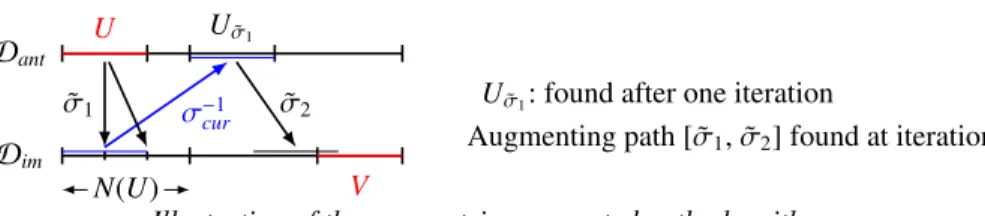
Dant Dim U Uσ˜1 N(U) V σ−1cur ˜ σ1 σ˜2
Illustration of the parametric augmented path algorithm Uσ˜1: found after one iteration
Augmenting path [ ˜σ1, ˜σ2] found at iteration 2
The algorithm builds an augmenting path by exploring the augmenting path tree of the bipartite graph in a breadth-first fashion. To improve the current mapping σ, we
need to get the actual augmenting path. The algorithm keeps track of the “potential starts” of augmenting paths in the list AP. If a pair (UAP ⊂ Dant,path) is added to AP (line 10), then we have found a set of paths starting from U, finishing at UAP, that are the starts of augmenting paths, and that use the partial bijections listed in path to go from Dantto Dim.
When we find an augmenting path, we actually find a (potentially parametric) set of augmenting paths, each of them non-mutually interfering (because σ and all the ˜σ are bijections), which can all be used together to improve σ. Also, keeping track of the partial bijections used in an augmenting path is enough information to characterize them: indeed, all the edges of an augmenting path going from Dimto Dantuse σ.
We also note that iterating on all the partial bijection can be done in constant non-parametric time: indeed, if we get a family of partial bijections ˜σtin the previous step,
we can still compute the image of a set through any ˜σtdirectly, instead of iterating over
all the values of t.
This algorithm is only able to find augmenting paths of non-parametric length. For example, we need N iterations of the algorithm to find the augmenting path in the fol-lowing graph: .. . ... 0 1 N −1 N 0′ 1′ N −1′ N′ : current σ : ˜σ1 U = {0}
Uexplorated(iteration i) = [|0; i|]
In summary, to combine the partial bijections into σ, we proceed as follows: first we use a greedy heuristic to quickly build a bijection. If the bijection is not total, then we try to improve it by using the augmenting path algorithm. There are three possible results to this algorithm: (i) a set of non-interfering augmenting paths is found, and we can improve our current bijection, (ii) our current σ is a maximum matching (thus, it is not possible to combine the partial bijections into a total bijection) or (iii) the algorithm does not terminate after an arbitrary number of iterations (there might be an augmenting path of parametric length, but we are not able to deal with this situation). While σ is not total, we keep applying the augmenting path algorithm.
5
Extensions
Sums of reductions The Decompose Reduce can be extended to sums of reductions: . . . ⊕ L πi(ki)=i Ei[ki] ⊕ . . . = . . . ⊕ L π′ i(k′i)=i ′ E′i[k′ i] ⊕ . . . E1[k1] = F1[k′1] En[kn] = Fm[k′m] σ(1, k1) = (1, k′1) σ(n, kn) = (m, k′m) . . . .
Because an occurrence of a given left reduction can be mapped to an occurrence to any right reduction, this rule is creating n × m sub-states, each one corresponding to all possible pairwise comparisons between the expressions. Moreover, we add one scalar dimension to the antecedent and image domains of σ: the value of this dimension corresponds to the reduction number in which the occurrence occurs. Thus, because each occurrence (α, kα) from the α-th left reduction will be mapped through σ to a
single occurrence of the β-th right reduction, all the other sub-states Eα = Eγ′ (where
γ , β) will become inaccessible for the index kα. That way, the bijection extraction will
naturally end up with a correct correspondence between the reductions.
This rule can be adapted to manage the associativity and commutativity of a fi-nite sum of non reduce expressions: indeed, we can use the following identity: E[i] =
L
Id(k)=i
E[k]. This ends up checking all possible equivalences between a left and a right expression, which is the idea to manage associativity and commutativity in Verdoolaege’s equivalence algorithm [13].
Reduction behind another reduction If we encounter a Decompose Reduce behind an-other Decompose Reduce, then the second bijection σ2might depend on the first
bijec-tion σ1. Thus, the derivation of both σ is related, and must not be separated. Instead of
deriving independently the constraints for each bijection, we can introduce σ = (σ1, σ2)
the bijection whose first dimensions correspond to σ1and last dimensions correspond
to σ2. The extracted constraints will deal with σ and the rest of the derivation algorithm
will apply. This result can be extended to any number of reduction, as soon as there is a finite non-parametric number of instances of σk(to be able to define σ).
6
Implementation
We have implemented a prototype of the equivalence algorithm4in Java, based on our
polyhedral compiler framework, AlphaZ. The implementation is still in progress: cur-rently we do not support loops behind a Decompose Reduction rule in the equivalence automaton, and we do not support our second extension (reduction behind another re-duction). We have run our implementation on several examples, and we report their corresponding execution time in Figure 2. Every example is managing parametric sum-mations, thus their equivalence cannot be decided by the previous works.
The Loop reverse example compares two 1D summation, one summing in increas-ing order and the other one in decreasincreas-ing order. The Distributed summation example compares two sums of reductions, summing the terms I[i] for 0 ≤ i < 2N differently. In the first sum, the terms are split across the two reductions according to the parity of
i. In the second sum, the terms are split between 0 ≤ i < N and N ≤ i < 2N. The Non
Equivalenceexample compares two reductions which are not equivalent (the second reduction has one extra term). The Tiling example compares a 1D summation (P
i
I[i]) with its tiled counterpart (P
ib P
il
I[16ib + il] where 0 ≤ il < 16).
Nstates Automaton Partial bijections Gathering Total exec. time Article (4.1) 15 74 206 133 414 Loop reverse 5 48 56 21 126 Distributed summation 15 75 788 297 1161 Non equivalence 4 45 48 84 179 Tiling 7 71 245 83 400
Fig. 2. Number of states in the equivalence automaton and execution time (in milliseconds). The machine running these experiments is composed of an Intel core i5-3210M and a Linux 3.2 kernel.
7
Conclusion
We have presented an extension to Barthou’s program equivalence semi-algorithm for SAREs to support the associativity and commutativity properties of reductions applied to parametric number of sub-terms. The key idea was to find a bijection σ which cor-rectly maps each expression of one reduction expression to a corresponding sub-expression of another reduction. We developed an algorithm to infer σ, and showed its relationship with the perfect matching problem in a parametric bipartite graph.
The idea of using and deriving a bijection can probably be used in other existing equivalence algorithms, such as the one by Verdoolaege et al. [13]. Some of these al-gorithms might take other program representation as input, such as affine control loop
programs. It is possible to translate such program by extracting the true dependences using techniques such as Array Dataflow Analysis [16]. Moreover, if the reductions are not provided, we need to use reduction detection techniques [17,18,19]. Also, there are probably links between the notions introduced in both algorithms, such as our accept
domainand their relation Rwantcorresponding to the (“desired correspondence between the iterations of both computations”).
About the parametric augmenting path algorithm, it might be possible to detect augmenting paths of parametric sizes if they present some regularity (such as periodicity of partial bijections). It would also be interesting to determine the maximum length of all the non-parametric augmenting paths: this number will be useful to determine the needed number of iterations of the while loop in our algorithm.
Our future plans involve the use of this algorithm to recognize instances of linear algebra algorithms (which often include reductions), with a goal to subsequently do “semantic tiling,” a program optimization technique that improves performance by ex-ploiting semantic properties. Finally, we would like to thank Alain Darte for helpful discussions.
References
1. Alias, C.: Program Optimization by Template Recognition and Replacement. PhD thesis, Université de Versailles (2005)
2. Godlin, B., Strichman, O.: Regression verification: Proving the equivalence of similar pro-grams. Software Testing, Verification and Reliability (2012)
3. Feng, X., Hu, A.J.: Cutpoints for formal equivalence verification of embedded software. In: 5th Intl Conf on Embedded Software (EMSOFT). (2005)
4. Hoare, T.: The verifying compiler: A grand challenge for computing research. J. ACM 50(1) (2003) 63–69
5. Necula, G.C.: Translation validation for an optimizing compiler. In: PLDI. (2000) 83–95 6. Pnueli, A., Siegel, M., Singerman, F.: Translation validation. In: TACAS, Springer (1998)
151–166
7. Zuck, L., Pnueli, A., Goldberg, B., Barrett, C., Fang, Y., Hu, Y.: Translation and run-time validation of loop transformations. Form. Methods Syst. Des. 27(3) (November 2005) 335– 360
8. Kundu, S., Tatlock, Z., Lerner, S.: Proving optimizations correct using parameterized pro-gram equivalence. In: PLDI 2009
9. Sangiorgi, D.: Bisimulation and coinduction. Cambridge (2012)
10. Janˇcar, P.: Decidability of bisimilarity for one-counter processes. Information and Compu-tation 158 (2000) 1–17
11. Barthou, D., Feautrier, P., Redon, X.: On the equivalence of two systems of affine recurrence equations (research note). In: Proceedings of the 8th International Euro-Par Conference on Parallel Processing. Euro-Par ’02, London, UK, UK, Springer-Verlag (2002) 309–313 12. Shashidhar, K.C., Bruynooghe, M., Catthoor, F., Janssens, G.: Verification of source code
transformations by program equivalence checking. In: Proceedings of the 14th International Conference on Compiler Construction. CC’05, Berlin, Heidelberg, Springer-Verlag (2005) 221–236
13. Verdoolaege, S., Janssens, G., Bruynooghe, M.: Equivalence checking of static affine pro-grams using widening to handle recurrences. ACM Trans. Program. Lang. Syst. 34(3) (November 2012) 11:1–11:35
14. Karfa, C., Banerjee, K., Sarkar, D., Mandal, C.: Verification of loop and arithmetic trans-formations of array-intensive behaviors. Computer-Aided Design of Integrated Circuits and Systems, IEEE Transactions on 32(11) (Nov 2013) 1787–1800
15. West, D.B.: Introduction to Graph Theory Introduction to Graph Theory (2nd Edition). Prentice Hall (1999)
16. Feautrier, P.: Dataflow analysis of array and scalar references. International Journal of Parallel Programming 20 (1991)
17. Redon, X., Feautrier, P.: Detection of scans in the polytope model. Parallel Algorithms and Applications 15 (2000) 229–263
18. Sato, S., Iwasaki, H.: Automatic parallelization via matrix multiplication. In: Proceedings of the 32Nd ACM SIGPLAN Conference on Programming Language Design and Implementa-tion. PLDI ’11, New York, NY, USA, ACM (2011) 470–479
19. Zou, Y., Rajopadhye, S.: Scan detection and parallelization in "inherently sequential" nested loop programs. In: Proceedings of the Tenth International Symposium on Code Generation and Optimization. CGO ’12, New York, NY, USA, ACM (2012) 74–83