Math 1: Analysis
Problems, Solutions and Hints
FOR THE ELECTRONICS AND TELECOMMUNICATION STUDENTS
Andrzej Ma´ckiewicz
Technical University of Pozna´n
Contents
1 Logic and techniques of proof (Exercises) 9
1.1 Practice Problems . . . 9
1.2 Exercises . . . 11
2 Introduction to limits (Exercises) 15 2.1 Basic concepts . . . 15
2.2 Examples . . . 18
2.3 Exercises . . . 20
3 Calculation of limits (Exercises) 23 3.1 Some basic, general facts about limits . . . 23
3.2 Practice Problems . . . 23
3.3 Some Trigonometric Limits . . . 28
3.3.1 Continuity of sine and cosine . . . 28
3.3.2 Tangent . . . 29
3.3.3 Cotangent . . . 29
3.3.4 Typical Examples . . . 30
3.4 The Epsilon-Delta Definition of a Limit . . . 31
3.5 Exercises . . . 33
4 Continuity (Exercises) 35 4.1 Continuous Functions . . . 35
4.1.1 Three types of "simple" discontinuities . . . 35
4.1.2 Classical continuous functions . . . 35
4.1.3 Several properties of continuous functions . . . 38
4.1.4 One sided continuity . . . 41
4.1.5 Continuity on an interval . . . 42
4.2 Exercises . . . 42
5 Benefits of Continuity (Exercises) 47 5.1 The Intermediate Value Theorem . . . 47
5.2 Boundedness; The Extreme Value Theorem . . . 52
6 The Derivative (Exercises) 55 7 How to solve differentiation problems (Exercises) 57
8 The derivative and graphs (Exercises) 59
8.1 Practice Problems . . . 59
8.1.1 Continuity and the Intermediate Value Theorem . . . . 59
8.1.2 Increasing and and Decreasing Functions . . . 61
8.1.3 The Second Derivative and Concavity . . . 62
8.2 Exercises. . . 64
9 Implicit differentiation 69 10 Sketching graphs (Exercises) 71 10.1 Practice Problems . . . 71
10.2 Exercises . . . 75
11 Optimization and linearization (Exercises) 77 11.1 Practice Problems . . . 77
11.2 Exercises . . . 81
11.3 Review exercises: Chapter 11 . . . 84
12 Definite integrals (Exercises) 93 12.1 Practice Problems . . . 93
12.1.1 The Definite Integral of a Continuous Function . . . 93
12.1.2 Indefinite integral . . . 95
12.2 Exercises . . . 98
13 The fundamental theorem of calculus (Exercises) 103 13.1 Practice Problems . . . 103
13.1.1 The Function F(x)=R () . . . 103
13.1.2 Area of a Region between 2 Curves . . . 105
13.1.3 The Area under an Infinite Region . . . 108
13.2 Exercises . . . 109
14 Natural logarithm (Exercises) 111 14.1 Practice Problems . . . 111
14.1.1 Properties of the natural logarithmic function . . . 111
14.1.2 Logarithmic differentiation . . . 112
14.2 Exercises . . . 112
Contents 5
15.1 Practice Problems . . . 113
15.2 Exercises . . . 113
16 Inverse functions and inverse trig functions (Exercises) 115 16.1 Practice Problems . . . 115
16.2 Exercises . . . 115
17 L’Hospital’s rule and overview of limits (Exercises) 117 17.1 Practice problems . . . 117
17.2 Exercises . . . 122
18 Applications of Integration (Exercises) 125 18.1 Practice Problems . . . 125
18.2 Exercises . . . 140
19 Arc Length and Surface Area (Exercises) 147 19.1 Practice Problems . . . 147
19.2 Exercises . . . 150
20 Techniques of integration, part one (Exercises) 153 20.1 Basic Integration Formulas . . . 153
20.2 Practice Problems . . . 153
20.2.1 Integration by substitution . . . 153
20.2.2 When substitution does not work . . . 156
20.3 Very Famous Example . . . 157
20.4 Exercises . . . 159
21 Techniques of integration, part two (Exercises) 165 21.1 Trigonometric Substitutions . . . 165
21.1.1 The Sine Substitution . . . 165
21.1.2 The Tangent Substitution . . . 167
21.1.3 Completing a square . . . 171
21.2 L’Hopital’s method and partial fractions . . . 173
21.3 Some famous examples . . . 176
21.4 Exercises . . . 179
22 Taylor polynomials (Exercises) 185 22.1 Practice Problems . . . 185
Preface
This is the complementary text to my Calculus Lecture Notes for the Elec-tronics and Telecommunication students at Technical University in Pozna´n. It is an outgrowth of my teaching of Calculus at Technical University of Pozna´n (for the first year students).
The goal of this text is to help students learn to use the most difficult parts of calculus intelligently in order to be able to solve a wide variety of mathematical and physical problems. The exercise sets have been carefully constructed to be of maximum use to the students.
Prerequisite material from algebra, trigonometry, and analytic geometry is consistent with the Polish standards. Students are advised to assess themselves and to take a pre-calculus course if they lack the necessary background.
The author de-emphasize the theory of limits, leaving a detailed study to the end of the course, after the students have mastered the fundamentals of calculus-differentiation and integration.
Computer and calculator applications are used for motivation and to illus-trate the numerical content of calculus. In my view the ability to visualize basic graphs and to interpret them mentally is very important in calculus and in subsequent mathematics courses.
This text leaves out the less important parts of the course because of the limited capacity of the book.
Misprints are a plague to authors (and readers) of mathematical textbooks. The author have made a special effort to weed them out, and we will be grateful to the readers who help us eliminate any that remain.
Andrzej Ma´ckiewicz Pozna´n, September 2014
1
Logic and techniques of proof (Exercises)
1.1
Practice Problems
Example 1 Prove that − has − as a factor for all positive integers .
Solution: The statement is true for = 1 since 1− 1 = − . Assume
the statement true for = , i.e., assume that − has − as a factor. Consider
+1− +1 = +1− + − +1 = ( − ) + (− )
The first term on the right has − as a factor, and the second term on the right also has − as a factor because of the above assumption. Thus +1− +1 has − as a factor if − does.¤
Example 2 If ∈ Z and ≥ 0, then P=0·! = ( + 1)! − 1 Solution: We will prove this with mathematical induction. 1) If = 0, this statement is
0
X
=0
·! = (0 + 1)! − 1
Since the left-hand side is 0·0! = 0, and the right-hand side is 1! − 1 = 0 the equationP0=0·! = (0 + 1)! − 1 holds, as both sides are zero. 2) Consider any integer ≥ 0. We must show that implies +1. That is,
we must show that
X =0 ·! = ( + 1)! − 1 implies +1 X =0 ·! = (( + 1) + 1)! − 1
We use direct proof. SupposeP=0·! = ( + 1)! − 1. Observe that +1 X =0 ·! = X =0 ·! + ( + 1) ( + 1)! = (( + 1)! − 1) + ( + 1) ( + 1)! = (1 + ( + 1)) ( + 1)! − 1 = ( + 2)! − 1 = (( + 1) + 1)! − 1 Therefore +1 X =0 ·! = (( + 1) + 1)! − 1 It follows by induction that
X
=0
·! = ( + 1)! − 1 for every integer ≥ 0.
Example 3 If ∈ N, then (1 + )≥ 1 + for all all ∈ R with −1. Solution: We will prove this with mathematical induction.
1) For the basis step, notice that when = 1 the statement is (1+)1 ≥ 1+1 , and this is true because both sides equal 1 +
2) Assume that for some ≥ 1, the statement (1 + ) ≥ 1 + is true for all all ∈ R with −1. From this we need to prove
(1 + )+1≥ 1 + ( + 1)
Now, 1 + is positive because −1, so we can multiply both sides of (1 + ) ≥ 1 + by (1 + ) without changing the direction of the inequality ≥.
(1 + )(1 + ) ≥ (1 + )(1 + ) (1 + )+1 ≥ 1 + + + 2 (1 + )+1 ≥ 1 + ( + 1) + 2
The above term 2 is positive, so removing it from the right-hand side
1.2 Exercises 11
1.2
Exercises
Exercise 1.1 The Fibonacci numbers {}∞=1 are defined by 1 = 2 = 1
and
+1= − −1 ≥ 2
Prove by induction that
=
¡
1 +√5¢+¡1 −√5¢
2√5 ≥ 1
Exercise 1.2 Thus, the first several Fibonacci numbers are 1 = 1; 2 = 1;
3 = 2; 4= 3; 5 = 5; 6 = 8; 7 = 13; 8 = 21; et cetera. Use
mathemat-ical induction to prove the following formula involving Fibonacci numbers.
X
=1
()2 = · +1
Exercise 1.3 Let the numbers 0 1 2 be defined by
0 = 1 1 = 3 = 4(−1− −2) for n ≥ 2
Show by induction that = 2−1( + 2) for all ≥ 0
Exercise 1.4 Prove by induction that
(1+ 2+ + )2 = X =1 2 + 2(12+ 13+ + 1+ 23 +24+ 2+ 34+ 35+ + −1)
Exercise 1.5 Prove by induction that
sin + sin 3 + sin 5 + + sin(2 − 1) = 1 − cos 22 sin for ≥ 1 HINT: You will need trigonometric identities that you can derive from the iden-tities
cos( − ) = cos cos + sin sin cos( + ) = cos cos − sin sin Take these two identities as given.
Exercise 1.6 Show that s 2 + r 2 + q 2 + √2 = 2 cos 2+1
where there are 2 in the expression on the left. HINT: We know that for any angle we have:
cos = r
1 + cos 2
2
Exercise 1.7 Prove by induction that, for all 6= 1 1 + 2 + 32+ + −1=
+1
− ( + 1)+ 1 ( − 1)2 Exercise 1.8 Prove by induction that for any positive integer
1 +1 2 + 1 3+ 1 4+ 1 5 + + 1 2−1 ≥ 1 2( + 1) HINT: Compare with Example (??).
Exercise 1.9 A “ postage stamp problem” is a problem that (typically) asks us to determine what total postage values can be produced using two sorts of stamps. Suppose that you have 3c/ stamps and 7c/ stamps, show (using strong induction) that any postage value 12c/ or higher can be achieved. That is,
for any ∈ N ≥ 12 ⇒ ∃ ∈ N = 3 + 7
Show that any integer postage of 12c/ or more can be made using only 4c/ and 5c/ stamps.
Exercise 1.10 Suppose that and are integers, with 0 ≤ ≤ . The binomial coefficient ¡¢ is the coefficient of in the expansion of (1 + ); that is, (1 + )= X =0 µ ¶ From this definition it follows immediately that
µ 0 ¶ = µ ¶ = 1 ≥ 0 For convenience we define
µ −1 ¶ = µ + 1 ¶ = 0 ≥ 0
1.2 Exercises 13 a) Show that µ + 1 ¶ = µ ¶ + µ − 1 ¶ 0 ≤ ≤ and use this to show by induction on that
µ ¶ = ! ! ( − )! 0 ≤ ≤ b) Show that X =0 (−1) µ ¶ = 0 and X =0 µ ¶ = 2 c) Show that ( + )= X =0 µ ¶ −
(This is the binomial theorem.) HINT: This is certainly true for = 1, since
( + )1 = + = µ 1 0 ¶ + µ 1 1 ¶ When = + 1 write ( + )+1 = ( + ) ( + ) = ( + ) X =0 µ ¶ − = X =0 µ ¶ +1−+ X =0 µ ¶ +1−
and replace by − 1 in the last sum to obtain ( + )+1 = +1+ X =1 ∙µ ¶ + µ − 1 ¶¸ +1− + +1
Finally, show how the right-hand side here becomes
+1+ X =1 µ + 1 ¶ +1− + +1 = +1 X =0 µ + 1 ¶ +1−
The identity µ ¶ + µ − 1 ¶ = µ + 1 ¶ ( ≥ ≥ 1)
is usually called the Pascal Triangle ldentity, since in the triangle of numbers 1 1 1 1 2 1 1 3 3 1 1 4 6 4 1 1 5 10 10 5 1
each “interior” entry is the sum of the two entries above it, and since the -th row turns out to be¡0¢¡1¢ ¡¢ Thus, if for example = 5 then directly from the Pascal’s triangle we have
( + )5 = 5+ 54 + 1032+ 1023+ 54+ 5
Exercise 1.11 Show that √3 and √3
2
Introduction to limits (Exercises)
2.1
Basic concepts
Suppose that a function has the graph shown below.
Our goal is to describe the behavior of in the vicinity of = 1 in a concise manner. Notice that (1) = 1 Yet, if ≈ 1 then () ≈ 2
So, the number 2 is crucial in describing the behavior of near 1 We say that 2 is the limit of () as approaches 1 This is written compactly as
lim
To be more precise, the reason that the limit is 2 as approaches 1 is that for any interval centered at 2 in the -axis (no matter how small) the number () will be in that interval for all other than 1 in some significantly small interval centered at = 1 in the -axis.
Also we point out, that lim→1 () has nothing to do with the value of at 1We can change (1) to any number we want, or even leave it undefined and the limit remains 2 Notice, that if lim→1 () = 2 is different than (1) there is a "hole" in the graph at (1 2)
If (1) were equal to 2, the "hole" would be filled. Value and limit coincide, whenever the graph of is continuous. This idea the basis of the mathematical definition of continuity (that will be presented later).
Let us look at another example. Again suppose that () has the graph shown below. Here the interesting behavior of is in the vicinity of = 0 Notice that (0) = 2 If ≈ 0 and 0 then () ≈ 2 But if ≈ 0 and 0 then () ≈ 1. Therefore, the limit of () as approaches 0 does not exist.
2.1 Basic concepts 17
However, we can say that 2 is the limit of () as approaches 0 from the left and express this by writing
lim
→0− () = 2
We can also say, that 1 is is the limit of () as approaches 0 from the right and express this by writing
lim
→0+ () = 2
Important fact:
lim→ () exists if and only if lim→− () and lim→+ ()
both exist and are equal.
If it happens, the common value of the one-sided limits is lim→ () Another example. Suppose, that () has the graph shown below.
Here the interesting behavior of is in the vicinity of = 2 Notice, that (2) is undefined and the line = 2 is a vertical asymptote. If ≈ 2 and 2, then () is large and positive. But if ≈ 2 and 2, then () is large and negative. Therefore, the limit of () as approaches 2 does not exist. In fact, neither of the one sided limits exist. However, we can describe the nature of the vertical asymptote writing:
lim
→2− () = +∞ and →2lim+ () = −∞
2.2
Examples
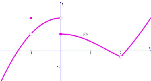
Example 4 Given the function () whose graph is below, determine the fol-lowing:
2.2 Examples 19
Solution:
a) (1) = 1 b) lim→1− () = 2
c) lim→1+ () = 0 d) lim→1 () does not exist.
¤
Example 5 Given the function whose graph is below, determine the follow-ing:
a) (2) b) lim→2− () c) lim→2+ () d) lim→2 ()
Solution:
a) (2) = 0 b) lim→2− () = 0
c) lim→2+ () = −∞ d) lim→2 () does not exist.
¤
Example 6 Sketch the graph of a function defined for −1 3 for which the following are true:
lim→−1+ () = 2 (0) = 1
lim→−0 () = 0 (1) = 0
lim→−1− () = ∞ lim→−1+ () = 1
(2) = 2 lim→−2+ () = 0
Solution: Here is a possible answer:
There are many other ways this graph could been drawn. Other possibilities need only indicate the correct values at, and limiting behavior near = −1 0 1 2 and 3.
2.3
Exercises
Exercise 2.1 Refer to the accompanying figure and determine the following: a) lim→2−() b) lim→2() c) lim→2+() d) lim→5()
2.3 Exercises 21
Exercise 2.2 Determine the one-sided limits of the function () in figure below, at the points = 1 3 5 6
Exercise 2.3 Use the graph of the function () to find the following a) lim→2− () b) lim→2 () c) lim→2+ () d) (2)
3
Calculation of limits (Exercises)
3.1
Some basic, general facts about limits
Some basic, general facts about limits are helpful in the calculation of specific limits.
Assume, that lim→ () and lim→() each exists. Then the following are true:
1. lim→( () + ()) = lim→ () + lim→() 2. lim→ () = lim→ ()
3. lim→( ()()) = (lim→ ()) (lim→()) 4. If lim→() 6= 0 then lim→ ()
() =
lim→ () lim→() 5. If lim→ () 6= 0 and lim→() = 0 then lim→ ()
() does not exist 6. If lim→ () = lim→() = 0 then lim→ ()
() may or may not exist
While these are stated in terms of the limit as approaches they are also true for one-sided limits as approaches
3.2
Practice Problems
We have the following limits regarding two specific simple functions lim→ = and lim→ =
Example 7 (a typical polynomial) lim →2 ¡ 23+ 3 + 5¢ = lim →22 3+ lim →23 + lim→25 = 2 lim →2 3+ 3 lim →2 + lim→25 = 2³lim →2 ´3 + 3 lim →2 + lim→25 = 2 (2)3+ 3 · 2 + 5 = 27
Notice that the result is simply the value of the polynomial at = 2. In fact, this always happens with polynomials, that is,
If () is a polynomial and is any real number, then lim→() = ()
¤
Example 8 (A rational function whose dominator does not approach zero). lim →3 22− + 2 2+ 1 = lim→3¡22− + 2¢ lim→3(2+ 1) = 2 (3) 2 − (3) + 2 (3)2+ 1 17 10
Again notice, that the result is simply the value of the function at = 3 In fact, this always happens with rational functions, provided that the denominator isn’t zero,
If () and () are polynomials, and () 6= 0 then lim→()
() = () () ¤
Example 9 (A rational function whose dominator approaches zero while its numerator does not).
lim
→1
22− + 2
3− 1 does not exist,
3.2 Practice Problems 25
Can we say something about one-sided limits? lim
→1−
22− + 2
3− 1 = −∞
as the nominator is close to 3 near 1, but the denominator ≈ 0 and 0 Similarly, lim →1+ 22− + 2 3− 1 = +∞ ¤
Recall the last of the six facts with which we began: 6. If lim→ () = lim→() = 0 then lim→ ()
() may or may not exist. It is the situation that is the most interesting and, in fact, is the main reason we are discussing limits at all!
Computation of limits in this " µ
0 0
" case often involves use of the following additional fact about limits:
7. If () = () for all near but not equal to then lim
→ () = lim→()
Here, think of () as a "simplified" version of () whose limit as → is easy to determine, such as polynomial or a rational function whose numerator and denominator do not both approach 0
Example 10 Find lim →1 3− 1 2− 1 Solution: 3− 1 2− 1 = ( − 1)¡ + 2+ 1¢ ( − 1) ( + 1) = ¡ + 2+ 1¢ ( + 1) for 6= 1 So, lim →1 3− 1 2− 1 = lim→1 ¡ + 2+ 1¢ ( + 1) = 12+ 1 + 1 1 + 1 = 3 2
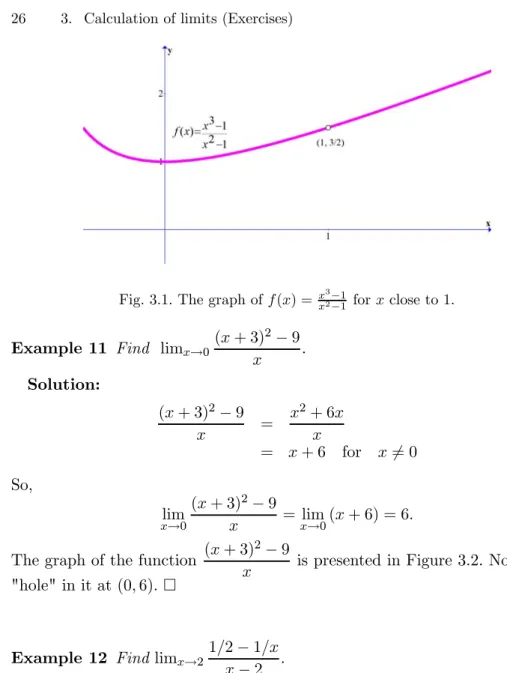
The graph of the function 32−1−1 is presented in Figure 3.1. Notice the "hole"
Fig. 3.1. The graph of () = 32−1−1 for close to 1
Example 11 Find lim→0 ( + 3)
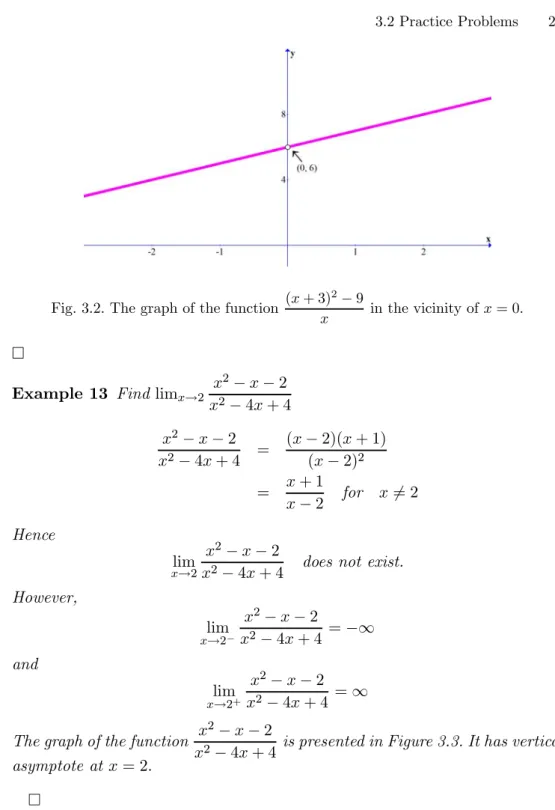
2 − 9 Solution: ( + 3)2− 9 = 2+ 6 = + 6 for 6= 0 So, lim →0 ( + 3)2− 9 = lim→0( + 6) = 6
The graph of the function ( + 3)
2
− 9
is presented in Figure 3.2. Notice the "hole" in it at (0 6)¤
Example 12 Find lim→2 12 − 1 − 2 Solution: 12 − 1 − 2 = − 2 2( − 2) = 1 2 for 6= 0 Hence, lim →2 12 − 1 − 2 = lim→2 1 2 = 1 4
3.2 Practice Problems 27
Fig. 3.2. The graph of the function ( + 3)
2
− 9
in the vicinity of = 0
¤
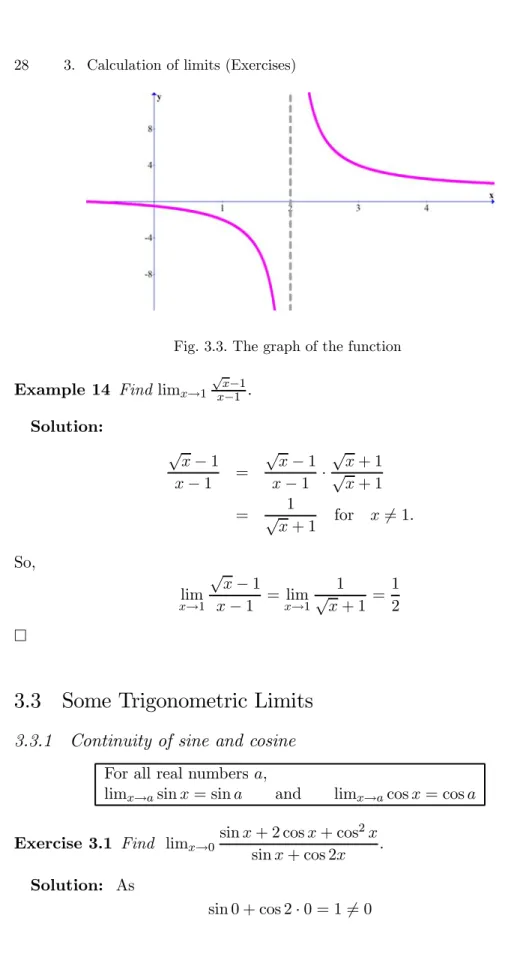
Example 13 Find lim→2
2 − − 2 2− 4 + 4 2− − 2 2− 4 + 4 = ( − 2)( + 1) ( − 2)2 = + 1 − 2 for 6= 2 Hence lim →2 2− − 2
2− 4 + 4 does not exist.
However, lim →2− 2− − 2 2− 4 + 4 = −∞ and lim →2+ 2− − 2 2− 4 + 4 = ∞
The graph of the function
2
− − 2
2− 4 + 4 is presented in Figure 3.3. It has vertical
asymptote at = 2 ¤
For the next example, we will need an additional continuity property lim→√ =√ for all 0 and lim→0+√ = 0
Fig. 3.3. The graph of the function
Example 14 Find lim→1
√ −1 −1 Solution: √ − 1 − 1 = √ − 1 − 1 · √ + 1 √ + 1 = √ 1 + 1 for 6= 1 So, lim →1 √ − 1 − 1 = lim→1 1 √ + 1 = 1 2 ¤
3.3
Some Trigonometric Limits
3.3.1
Continuity of sine and cosine
For all real numbers ,
lim→sin = sin and lim→cos = cos
Exercise 3.1 Find lim→0 sin + 2 cos + cos
2
sin + cos 2 Solution: As
3.3 Some Trigonometric Limits 29
lim
→0
sin + 2 cos + cos2 sin + cos 2 =
lim→0¡sin + 2 cos + cos2¢ lim→0(sin + cos 2) = sin 0 + 2 cos 0 + cos
20
sin 0 + cos 2 · 0 = 3
¤
3.3.2
Tangent
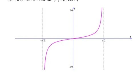
If is not an odd multiple of 2 then cos 6= 0 and so lim →tan = lim→ sin cos = sin cos = tan
Suppose that is an odd multiple of 2 Then sin 6= 0 and cos = 0 so lim→tan does not exist.
If ≈ and then sin and cos have the same sign; so tan 0 Therefore
lim
→−tan = lim→−
sin cos = ∞
If ≈ and then sin and cos have opposite sign; so tan 0 Therefore lim →+tan = lim→+ sin cos = −∞
3.3.3
Cotangent
If is not a multiple of then sin 6= 0 and so lim →cot = lim→ cos sin = cos sin = cot If is a multiple of then lim→cot does not exist.
Note that
cot = tan³ 2 −
´
= − tan³ −2´ So, if is a multiple of then
lim
→−cot = − lim→−tan
³ − 2 ´ = − lim →(− 2) −tan = −∞ and similarly lim
→+cot = − lim→+tan
³
−2´= − lim
→(−2)
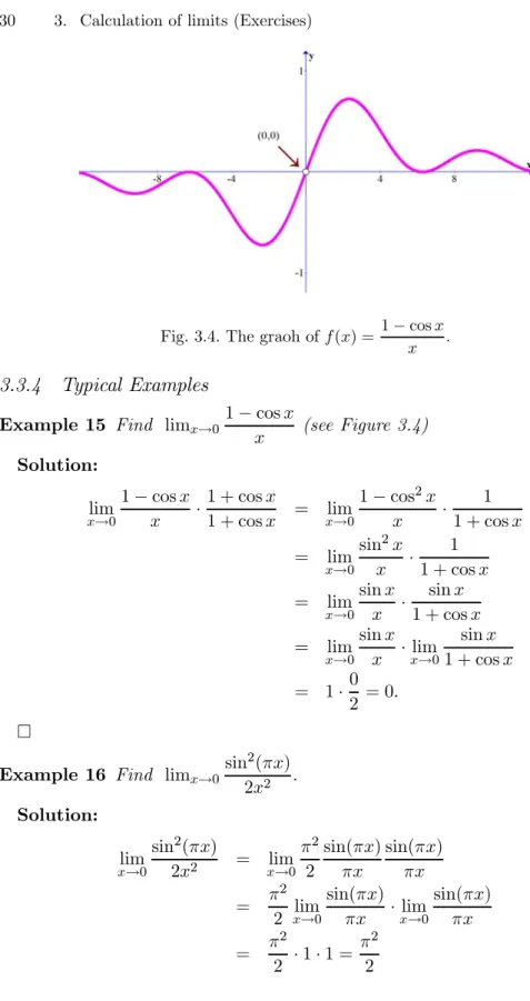
Fig. 3.4. The graoh of () = 1 − cos
3.3.4
Typical Examples
Example 15 Find lim→0 1 − cos
(see Figure 3.4) Solution: lim →0 1 − cos · 1 + cos 1 + cos = →0lim 1 − cos2 · 1 1 + cos = lim →0 sin2 · 1 1 + cos = lim →0 sin · sin 1 + cos = lim →0 sin · lim→0 sin 1 + cos = 1 · 02 = 0 ¤
Example 16 Find lim→0 sin
2() 22 Solution: lim →0 sin2() 22 = →0lim 2 2 sin() sin() = 2 2 →0lim sin() · lim→0 sin() = 2 2 · 1 · 1 = 2 2
3.4 The Epsilon-Delta Definition of a Limit 31
¤
Example 17 Find lim→0 2 − 3 cos + cos
2 sin Solution: lim →0 2 − 3 cos + cos2 sin = →0lim (2 − cos ) (1 − cos ) sin = lim →0(2 − cos ) (1 − cos ) sin = (2 − 1) · 01 = 0 ¤
Example 18 Find lim→0 1 − cos(3) 2 Solution: lim →0 1 − cos(3) 2 = →0lim 1 − cos(3) 2 · 1 + cos(3) 1 + cos(3) = lim →0 1 − cos2(3) 2 · 1 1 + cos(3) lim →0 sin(3) · sin(3) 3 · 3 1 + cos(3) = 1 · 1 ·92 = 9 2 ¤
3.4
The Epsilon-Delta Definition of a Limit
Let be a function that is defined on an open interval containing except possibly itself, and let be a real number. The statement
lim→ () =
means that for every 0 there exists a 0 such that if 0 | − | then |() − |
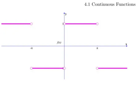
Solution: If 0 then || = = 1 and hence, to the right of the -axis, the graph coincides with the line = 1 If 0 then || = − = −1 which means that to the left of the -axis the graph of coincides with the line = −1 If it were true that lim→0 () = for sone then the preceding
remarks imply, that −1 ≤ ≤ 1 If we consider any pair of horizontal lines = ± where 1 0 then there exist points on the graph which are not between these lines for some nonzero in every interval (− ) containing 0 It follows that the limit does not exist.¤
Example 20 For the limit given below, find the largest that works for the given
lim
→42 = 8 = 01
Solution: The definition tells us that lim→42 = 8 iff for each 0 there exists a 0 such that
if 0 | − 4| then |2 − 8|
Note that |2 − 8| = 2 | − 4| Thus |2 − 8| whenever 2 | − 4| or | − 4| 2 From the work shown above, we see that the largest choice of
that works for 0 is = 2¤
Exercise 3.2 Give an − proof for the following limit lim
→3(3 + 1) = 10
Solution: The definition tells us that lim→3(3 + 1) = 10 iff for each 0 there exists a 0 such that
if 0 | − 3| then |(3 + 1) − 10| Note that
|(3 + 1) − 10| = |3 − 9| = 3 | − 3|
Thus |(3 + 1) − 10| whenever 3 | − 3| or | − 3| 3 Now let 0 Choose = 3
If 0 | − 3| then
|(3 + 1) − 10| = |3 − 9| = 3 | − 3| 3 = 3³ 3´= By the − definition of a limit, lim→3(3 + 1) = 10 ¤
3.5 Exercises 33
3.5
Exercises
Exercise 3.3 Why is it impossible to investigate lim→0√ by means of the Epsilon-Delta Definition of a Limit.
Exercise 3.4 For the limit given below, find the largest that works for the given lim →4 1 5 = 4 5 = 001 Answer: = 005
Exercise 3.5 Give an − proof for the following limit lim
→2(6 − 4) = −2
Exercise 3.6 Give an − proof for the following limit lim
4
Continuity (Exercises)
4.1
Continuous Functions
Let be a function whose domain includes an open interval centered at = Then is said to be continuous at if
lim→ () = ()
Example 21 Let’s () be the function with the graph presented in Figure 4.1 Then
• is continuous everywhere except at = −1 0 and 2
• is not continuous at −1 because lim→−1 () = 1 while (−1) = 2
• is not continuous at 0 because lim→0 () does not exist.
• is not continuous at 2 because (2) is not defined.
4.1.1
Three types of "simple" discontinuities
Example 22 Let’s () be the function with the graph presented in Figure 4.2 Then it has
• "Jump" discontinuity at = −1 (one-sided limits exist but are different). • "Infinite" discontinuity at = 0 (An infinite one-sided limit).
• "Removable" discontinuity (the limit exists but does not equal the value of function)
4.1.2
Classical continuous functions
• Polynomials are continuous everywhere.
• Rational functions are continuous whenever they are defined. • sin and cos are continuous everywhere.
Fig. 4.1. The graph of an exemplary function ()
4.1 Continuous Functions 37
• tan cot sec , and csc are continuous whenever they are defined. Example 23 The rational function
() = ( − 1)(2 + 1) ( − 1)
has only two discontinuity points at 1. = 0 ("Infinite" discontinuity). 2. = 1 ("Removable" discontinuity).
Example 24 The function f(x) = sin() is continuous everywhere except at = 0. It is a prototype of a function which is not continuous due to os-cillation. We can approach = 0 in ways that () = 1 and such that
4.1.3
Several properties of continuous functions
Directly from the properties of the limits it follows that If and are both continuous at then
1. + and − are continuous at 2. is continuous at
3. is continuous at
4. if () 6= 0 then is continuous at Compositions
5. if is continuous at and is continuous at () then ◦ is continuous at Example 25 Let () = 32+ 2 − 1 ( − 1)( − sin )
At what values of is not continuous? Of what type is each of its disconti-nuities?
Solution: First observe, that 32, 2− 1, and ( − 1)( − sin ) are each
continuous everywhere, since they involve only polynomials and sine. There-fore, is continuous whenever (−1)(−sin ) 6= 0, that is, everywhere except at = 1 and = 0
To determine the type of discontinuity at = 1, we will examine lim→1 ()
() = 32+ 2 − 1 ( − 1)( − sin ) = 3 2+ + 1 ( − sin ) for 6= 1
4.1 Continuous Functions 39
So, the limit exists: lim
→1 () = 3 · 1 +
1 + 1
(1 − sin 1) ≈ 15 616
Therefore, the discontinuity at = 1 is removable, corresponding to a "hole" in the graph of
To determine the type of discontinuity at = 0, we first notice that lim
→0 () does not exist
and in fact
lim
→0− () = −∞ and →0lim+ () = ∞
Therefore, has an infinite discontinuity at = 0 corresponding to a vertical asymptote.¤
Example 26 Find numbers and such that the following function is con-tinuous everywhere () = ⎧ ⎪ ⎪ ⎪ ⎪ ⎨ ⎪ ⎪ ⎪ ⎪ ⎩ if ≤ 1 2+ − if −1 ≤ 1 if 1 ≤
Solution: Since the "parts" of are polynomials, we only need to choose and so that is continuous at = −1 and 1 we have
lim →−1− () =→−1lim+ () = (−1) lim →−1− =→−1lim+ 2 + − = (−1) − = 1 + − −2 + = 1 and lim →1− () = lim→1+ () = (1) lim →1− 2 + − = lim →1+ 1 + − =
Fig. 4.3. Continuous function from Example 26
− 2 = −1 Solving the system of two linear equations
⎧ ⎨ ⎩ −2 + = 1 − 2 = −1 which is equivalent to −3 = −1 − 23 = −1 we get = −13 = 1 3 (see Figure 4.3) ¤
Example 27 (Composition) Let
() = || = ⎧ ⎨ ⎩ −1 if 0 1 if ≥ 0 If we compose with sin the result
() = sin |sin |
will be continuous, whenever sin 6= 0 i.e. except multipliers of At multi-pliers of it is undefined and has a jump discontinuity (see Figure 4.4).
4.1 Continuous Functions 41
Fig. 4.4. Function () = |sin |sin
4.1.4
One sided continuity
If the domain of includes an interval whose right endpoint is then is left continuous at if
lim
→− () = ()
If the domain of includes an interval whose left endpoint is then is right continuous at if
lim
→+ () = ()
Function () is continuous at if and only if is both left continuous and right continuous at Example 28 lim →+ √ =√ for all 0 and lim →0+ √ = 0
So square root function is continuous at every positive number and right con-tinuous at 0
4.1.5
Continuity on an interval
Let be an interval i.e., a set of one of the following forms
( ) [ ] [ ) ( ] ( ∞) (−∞ ) (−∞ ] or (−∞ ∞) A function whose domain includes is said to be continuous on if for every number in
• is continuous at if is not an endpoint of • is right continuous at if is a left endpoint of • is left continuous at if is a right endpoint of
If the domain of is an interval, and if is continuous on that interval, then we may simply say that is a continuous function.
Example 29 a) () = 1 is continuous on (0 ∞) and on (−∞ 0) b) () =√ is continuous on [0 ∞) c) () =√1 − 2 is continuous on [−1 1)
4.2
Exercises
Exercise 4.1 Let () = ⎧ ⎨ ⎩ 2 + 1 if ≤ 1 2− 1 if 14.2 Exercises 43
Fig. 4.5. Function () =√1 − 2
Is continuous at = 1? If not, what type of discontinuity does have at = 1?
Answer: The function is discontinuous at = 1 and has jump disconti-nuity there. Exercise 4.2 Let () = ⎧ ⎨ ⎩ 2 + 1 if ≤ 1 0 if = 1 2+ 2 if 1
Is continuous at = 1? If not, what type of discontinuity does have at = 1?
Answer: The function is discontinuous at = 1 and has removable dis-continuity there. Exercise 4.3 Let () = ⎧ ⎨ ⎩ 2 + 1 if ≤ 1 0 if = 1 1 −1 if 1
Is continuous at = 1? If not, what type of discontinuity does have at = 1?
Answer: The function is discontinuous at = 1 and has infinite discon-tinuity there. Exercise 4.4 Let () = ⎧ ⎨ ⎩ 22 if ≤ 2 (1 − ) if 2 For what values of is continuous at = 2?
Answer: = 12 or = −1 Exercise 4.5 Let () = √ + 4 − 3 √ − 5
If possible define at = 5 so that is continuous at = 5 Answer: (5) = 0.
Exercise 4.6 The graph of the function is shown in the figure below. De-termine the intervals on which is continuous.
Answer: (−2 −1] (−1 1) [1 2] Exercise 4.7 Let () = ⎧ ⎨ ⎩ + 1 if ≤ 1 1 −1 if 1
Determine the intervals on which is continuous. Answer: (−∞ 1) (1 ∞) Exercise 4.8 Let () = ⎧ ⎨ ⎩ −2 if ≤ −1 || if −1 1 1 −1 if ≥ 1
Determine the intervals on which is continuous. Answer: (−∞ 1] (1 ∞)
4.2 Exercises 45 Exercise 4.9 Let () = ⎧ ⎨ ⎩ −2 if ≤ −1 || if −1 1 1 −1 if ≥ 1
a) Sketch the graph of
b) At which points is discontinuous?
c) For each point of discontinuity found in b) determine whether is contin-uous from the right, from the left, or neither.
d) Classify each discontinuity found in b) as being a removable discontinuity, jump discontinuity, or an infinite discontinuity.
5
Benefits of Continuity (Exercises)
5.1
The Intermediate Value Theorem
Theorem 30 (The Intermediate Value Theorem) Suppose () is con-tinuous on the interval [ ] and let 0 be a number between () and ()
Then there exists a number in ( ) such that () = 0
Example 31 Use the Intermediate Value Theorem to show that there is a solution of the given equation in the indicated interval
5− 24− − 3 = 0 [23] Solution:
Scratch Work:
To show that the equation 5−24−−3 = 0 has a solution on the interval [23], follow the steps below:
1. Let () = 5− 24− − 3 Observe, that is continuous on [23]
Fig. 5.1. The equation 5− 24− − 3 = 0 has a solution in [23]
3. Note that = 0 is the number between (2) and (3)
4. is continuous on [2 3] and 0 is a number between (2) and (3). So, use the Intermediate Value Theorem to conclude that there is at least one number in the interval (2 3) such that () = 0
Let () = 5−24−−3 Since is a polynomial function, it is continuous on the closed interval [2 3] Now, (2) = −5 and (3) = 7 Thus (2) 0 (3). Hence , = 0 is a number between (2) and (3) By the Intermediate Value Theorem, there is at least one number in the interval (2 3) such that () = 0 Therefore, the equation 5− 24− − 3 = 0 has a solution in the interval [23] (see Figure 5.1).¤
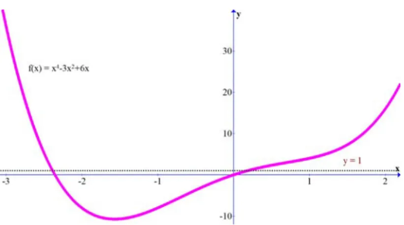
Example 32 Let
() = 4− 32+ 6 show that there is a number such that () = 1
Solution: Let () = 4− 32+ 6 Since is a polynomial function, it is continuous on the closed interval [−3 −2] Now, (−3) = 36 and (−2) = −8 Thus, (−2) 1 (−3) Hence, = 1 is a number between (−3) and (−2) By the Intermediate Value Theorem, there is at least one number in the interval (−3 −2) such that () = 1 (see Figure 5.2) ¤
Example 33 Solve the given inequality for 2− 3
5.1 The Intermediate Value Theorem 49
Fig. 5.2. The graph of the function () = 4− 32+ 6
Solution: Let () = 2 − 3 + 1 Since () = ( − 3) + 1
we see that () = 0 for = 0 and = 3 Also, () is not defined at = −1 The numbers −1 0 and 3 partition the real line into 4 subintervals
(−∞ −1) (−1 0) (0 3) and (3 ∞)
The rational function () = (−3)+1 is continuous and nonzero on each of these intervals. Therefore, either () 0 or () 0 on each of the subintervals. To determine the sign of () on each interval, choose a number in each subinterval and evaluate ()
• Choose = −2 on the subinterval (−∞ −1) (−2) = −10 so () 0 on the subinterval (−∞ −1) • Choose = −12 on the subinterval (−1 0)
(−12) = 7 2 so () 0 on the subinterval (−1 0)
• Choose = 1 on the subinterval (0 3) (1) = −1 so () 0 on the subinterval (0 3) • Choose = 4 on the subinterval (3 ∞)
(4) = 4 5
so () 0 on the subinterval (3 ∞) Therefore, the solution set of the inequality 2+1−3 0 is (−∞ −1) ∪ (0 3)
¤
Example 34 At 8 : 00 A.M. on Saturday a man begins running up the side of a mountain to his weekend campsite (see figure). On Sunday morning at 8 : 00 A.M. he runs back down the mountain. It takes him 20 minutes to run up, but only 10 minutes to run down. At some point on the way down, he realizes that he passed the same place at exactly the same time on Saturday. Prove that he is correct.
5.1 The Intermediate Value Theorem 51
Solution: HINT: Let () and () be the position functions for the runs up and down, and apply the Intermediate Value Theorem to the function () = () − ()
Example 35 Verify that the function () = 17− 3+ 5+ 57+ sin() has
a root.
Solution: The function goes to +∞ for → ∞ and to −∞ for → −∞. We have for example (10000) 0 and (−1000000) 0. The intermediate value theorem assures there is a point where () = 0.¤
Example 36 There is a point on the earth, where temperature and pressure agrees with the temperature and pressure on the antipode.
Solution: Lets draw a meridian through the north and south pole and let () be the temperature on that circle. Define () = () − ( + ). If this function is zero on the north pole, we have found our point. If not, () has different signs on the north and south pole. There exists therefore an , here the temperature is the same. Now, for every meridian, we have a latitude value () for which the temperature works. Now define () = () − ( + ). This function is continuous. Start with meridian 0. If (0) = 0 we have found our point. If not, then (0) and () take different signs. By the intermediate value theorem again, we have a root of . At this point both temperature and pressure are the same than on the antipode. Remark: this argument in the second part is not yet complete. Do you see where the problem is?
Fig. 5.3. Function () which is continuous on (−2 2) but has no minimum value, and has no maximum value.
5.2
Boundedness; The Extreme Value Theorem
Theorem 37 (The Extreme Value Theorem) Suppose that is contin-uous on a closed bounded interval [ ]. Then there exist numbers and in [ ] such that
() ≤ () ≤ () for all in [ ]
Example 38 Give an example of a function which is continuous on an open interval ( ), but it has no minimum value and it has no maximum value
Solution: See Figure 5.3
Example 39 Give an example of a function which is defined but not con-tinuous on an closed interval [ ], but it has no minimum value.
Solution: Figure 5.4 presents such a function.
5.3
Exercises
Exercise 5.1 Given that and are continuous on [ ] such that () () and () (), prove that there is a number in ( ) such that () = ()
Exercise 5.2 Prove that the equation 2+ 1
+ 3 + 4+ 1
5.3 Exercises 53
Fig. 5.4. This function has no minimum value on [0 2]
has a solution in the interval (−3 4)
Exercise 5.3 Show, that there is a solution to the equation = 10.
Exercise 5.4 Does the function () = + ln | ln ||| have a root somewhere? Exercise 5.5 Prove that on an arbitrary floor, a square table can be turned so that it does not wobble any more.
Exercise 5.6 Sketch the graph of a function that is defined on the interval [1 2] and meets the given conditions (if possible).
a) is continuous on [1 2]
b) The maximum value of on [1 2] is 3 c) The maximum value of on [1 2] is 1
Exercise 5.7 Sketch the graph of a function that is defined on the interval [1 2] and meets the given conditions (if possible).
a) is continuous on (1 2)
b) The function takes only three distinct values.
Exercise 5.8 Sketch the graph of a function that is defined on the interval [1 2] and meets the given conditions (if possible).
a) is continuous on (1 2)
b) the range of is an unbounded interval
Exercise 5.9 Sketch the graph of a function that is defined on the interval [1 2] and meets the given conditions (if possible).
a) is continuous on [1 2]
6
7
How to solve differentiation problems
(Exercises)
8
The derivative and graphs (Exercises)
Differential calculus provides tests for locating the key features of graphs.
8.1
Practice Problems
8.1.1
Continuity and the Intermediate Value Theorem
If a continuous function on a closed interval has opposite signs at the end-points, it must be zero at some interior point.
Example 40 Show that the function () = ( − 1)32 is continuous at 0 = 4.
Solution: This is a rational function whose denominator does not vanish at 0 = 4, so it is continuous by the rational function rule.¤
Example 41 Let () be the step function defined by
() = ⎧ ⎨ ⎩ 0 if ≤ 0 1 if 0 Show that is not continuous at 0 = 0. Sketch.
Solution: The graph of g is shown in Fig. 8.1. Since approaches (in fact, equals) 0 as approaches 0 from the left, but approaches 1 as approaches 0 from the right, lim→0() does not exist. Therefore, is not continuous at 0 = 0. ¤
We proved the following theorem: is differentiable at 0, then is
con-tinuous at 0. Using our knowledge of differential calculus, we can use this
relationship to establish the continuity of additional functions or to confirm the continuity of functions originally determined using the laws of limits. Example 42
a) Show that () = 32(3− 2) is continuous at 0 = 1. Where else is it
Fig. 8.1. This step function is discontinuous at 0= 0.
b) Show that () =√2+ 2 + 1 is continuous at = 0.
Solution:
a) By our rules for differentiation, we see that this function is differentiable at 0 = 1; indeed, 3 − 2 does not vanish at 0 = 1. Thus is also
continuous at 0 = 1. Similarly, is continuous at each , such that
3− 2 6= 0, i.e., at each 6=√3
2.
b) This function is the composition of the square root function () = √ and the function () = 2+ 2 + 1; () = (()). Note that (0) = 1 0. Since is differentiable at any (being a polynomial), and is differentiable at = , is differentiable at = 0 by the chain rule. Thus is continuous at = 0. ¤
A continuous function is one whose graph never "jumps." The definition of continuity is local since continuity at each point involves values of the function only near that point. There is a corresponding global statement, called the Intermediate Value Theorem, which involves the behavior of a function over an entire interval [ ].
Example 43 Show that there is a number , such that 50− 0 = 3.
Solution: Let () = 5− . Then (0) = 0 and (2) = 30. Since 0 3 30, the intermediate value theorem guarantees that there is a number 0, in
(0 2) such that (0) = 3. (The function is continuous on [0 2] because it
is a polynomial.) ¤
Notice that the intermediate value theorem does not tell us how to find the number 0, but merely that it exists. (In fact there may be more than one
8.1 Practice Problems 61
possible choice for 0.) Nevertheless, by repeatedly dividing an interval into
two or more parts and evaluating () at the dividing points, we can solve the equation (0) = as accurately as we wish. This method of bisection is
illustrated in the next example.
Example 44 (The method of bisection) Find a solution of the equation 5− = 3 in (0 2) to within an accuracy of 01 by repeatedly dividing intervals in half and testing each half for a root.
Solution: In Example 43 we saw that the equation has a solution in the interval (0 2). To locate the solution more precisely, we evaluate (1) = 15− 1 = 0. Thus (1) 3 (2), so there is a root in (1 2). Now we bisect
[1 2] into [1 15] and [15 2] and repeat: (15)w 609 3. so there is a root in (1 15); (125) = 180 3, so there is a root in (125 15); f(1.375)w 354 3, so there is a root in (125 1375); thus 0 = 13 is within 01 of a root. Further
accuracy can be obtained by means of further bisections. ¤
8.1.2
Increasing and and Decreasing Functions
The sign of the derivative indicates whether a function is increasing or de-creasing.
Example 45 Show that () = 2 is increasing at 0 = 2.
Solution: Choose ( ) to be, say, (1 3). If 1 2, we have () = 2 4 = 20. If 2 3, then () = 2 4 = 20. We have verified conditions of the definition, so is increasing at 0= 2. ¤
Example 46
a) Is 5− 3− 22 increasing or decreasing at −2? b) Is () =√2− increasing or decreasing at = 2?
Solution:
a) Letting () = 5−3−22, we have 0() = 54−32−4, and 0(−2) = 5(−2) −3(−2)2 − 4(−2) = 80 − 12 + 8 = 76, which is positive. Thus 5− 3− 22 is increasing at −2.
b) By the chain rule, 0() = 12√2−1
2− so 0(2) = 3 4 √ 2 0. Thus is increasing at = 2. ¤
Solution: Notice that (−1) = 0. Also, 0(−1) = 3(−1)2 − 2(−1) +1 = 6
0, so is increasing at = −1 Thus changes sign from negative to positive. ¤
Example 48 On what intervals is () = 3−2+6 increasing or decreasing? Solution: We consider the derivative 0() = 32 − 2. This is positive
when 32− 2 0, i.e., when 2 23, i.e., either p23 or −p23. Similarly, 0() 0 when 2 23, i.e., −p23 p23. Thus, is increasing on the intervals (−∞ −p23) and (p23 ∞) , and is decreasing on (−p23p23). ¤
Example 49 Match each of the functions in the left-hand column of Fig. 8.2 with its derivative in the right-hand column.
Solution: Function (1) is decreasing for 0 and increasing for 0. The only functions in the right-hand column which are negative for 0 and positive for 0 are () and (). We notice, further, that the derivative of function 1is not constant for 0 (the slope of the tangent is constantly changing), which eliminates (). Similar reasoning leads to the rest of the answers, which are: () − () (2) − () (3) − () (4) − () (5) − ().
Exercise 8.1 Find the critical points of the function () = 34−83+62− 1. Are they local maximum or minimum points?
Solution: We begin by finding the critical points:
0() = 123− 242+ 12 = 12(2− 2 + 1) = 12( − 1)2;
the critical points are thus 0 and 1. Since ( − 1)2 is always nonnegative, the only sign change is from negative to positive at 0. Thus 0 is a local minimum point, and is increasing at 1 (see Fig. 8.3). ¤
8.1.3
The Second Derivative and Concavity
The sign of the second derivative indicates which way the graph of a function is bending.
Example 50 Find the intervals on which () = 33 − 8 + 12 is concave upward and on which it is concave downward. Make a rough sketch of the graph.
Solution: Differentiating , we get 0() = 92−8, 00() = 18. Thus is concave upward when 18 0 (that is, when 0 ) and concave downward
8.1 Practice Problems 63
Fig. 8.2. Matching functions and their derivatives.
Fig. 8.4. The critical points and concavity of () = 33− 8 + 12
when 0. The critical points occur when 0() = 0, i.e., at = ±p89 = ±
2 3 √ 2. Since 00(−2 3 √ 2) 0, −23 √
2 is a local maximum, and since ”(23√2) 0 , 23√2 is a local minimum. Additionaly = 0 is an inflection point for , as 00(0) = 0 This information is sketched in Fig. 8.4 ¤
Example 51 Find the inflection points of the function () = 244− 323+ 92+ 1.
Solution: We have 0() = 963− 962+ 18, so 00() = 2882− 192 + 18, Solution is: 121√7 + 1313 − 121√7. To find inflection points, we begin by solving 00() = 0; the quadratic formula gives = ¡13 ±121√7¢. Using our knowledge of parabolas, we can conclude that 00 changes from positive to negative at ¡13− 121√7¢ and from negative to positive at ¡13 +121 √7¢; thus both are inflection points.
8.2
Exercises.
Exercise 8.2 Suppose that is continuous on [0 3], that has no roots on the interval, and that (0) = 1. Prove that () 0 for all x in [0 3].
Exercise 8.3 Where is () = 92− 3√4− 22− 8 continuous?
Exercise 8.4 Show that the equation −5+ 2 = 2 − 6 has a real solution. Exercise 8.5 Prove that () = 8+ 34− 1 has at least two distinct (real) zeros.
8.2 Exercises. 65
Fig. 8.5. Sketch functions that have these derivatives..
Exercise 8.6 Find all points in which () = 2− 3 + 2 is increasing, and at which it changes sign.
Exercise 8.7 Find a quadratic polynomial which is zero at = 1, is decreas-ing if 2, and is increasdecreas-ing if 2.
Exercise 8.8 Sketch functions whose derivatives are shown in Fig. 8.5.
Exercise 8.9 Find the inflection points for the following functions:
a) () = 3−
b) () = 7
Exercise 8.10 Match the graphs of the functions () in ) − ) with 00()
8.2 Exercises. 67
Exercise 8.11 Match the following functions ) − ) with their second deriv-atives 1) − 8):
Exercise 8.12 Match the functions (-) (top row) with their derivatives (1-4) (middle row) and second derivatives (-) (last row).
9
10
Sketching graphs (Exercises)
Using calculus to determine the principal features of a graph often produces better results than simple plotting.
Graphing procedure:
To sketch the graph of a function :
1. Note any symmetries of . Is () = (−), or () = −(−), or neither? In the first case, is called even; in the second case, is called odd. If is even that is, () = (−) we may plot the graph for ≥ 0 and then reflect the result across they axis to obtain the graph for ≤ 0. If is odd, that is, () = −(−) then, having plotted for ≥ 0, we may reflect the graph in the axis and then in the axis to obtain the graph for ≤ 0.
2. Locate any points where is not defined and determine the behavior of near these points. Also determine, if you can, the behavior of () for very large positive and negative.
3. Locate the local maxima and minima of , and determine the intervals on which is increasing and decreasing.
4. Locate the inflection points of , and determine the intervals on which is concave upward and downward.
5. Plot a few other key points, such as and intercepts, and draw a small piece of the tangent line to the graph at each of the points you have plotted. (To do this, you must evaluate 0() at each point.)
6. Fill in the graph consistent with the information gathered in steps 1 through 5
10.1
Practice Problems
Example 52 Sketch the graph of () = 1 + 2
Solution: We carry out the six-step procedure:
1. (−) = −¡1 + (−)2¢ = −¡1 + ()2¢ = −(); is odd, so its graph must by symmetric when reflected in the and axes.
2. Since the denominator 1 + 2 is never zero, the function is defined every-where; there are no vertical asymptotes. For 6= 0, we have
() = 1 + 2 =
1 + 1
Since becomes small as becomes large, () looks like 1( + 0) = for large. Thus = 0 is a horizontal asymptote; the graph is below = 0 for large and negative and above = 0 for large and positive. 3. 0() = 1 2+ 1− 2 2 (2+ 1)2 = ¡ 1 − 2¢ (2+ 1)2
which vanishes when = ±1 . To check the sign of 0() on (−∞ −1), (−1 1), and (1 ∞), we evaluate it at conveniently chosen points: 0(−2) = −325 0(0) = 1 0(2) = −325 . Thus is decreasing on (−∞ −1) and on (1 ∞) and is increasing on (−1 1). Hence −1 is a local mini-mum and 1 is a local maximini-mum by the first derivative test.
4. 00() = 8 3 (2+ 1)3 − 6 (2+ 1)2 = 2 (2+ 1)3 ¡ 2− 3¢
This is zero when = 0√3 and −√3. Since the denominator of 00 is positive, we can determine the sign by evaluating the numerator. Evalu-ating at −2 −1 1 and 2, we get −4, 4, −4, and 4, so is concave down-ward on ¡−∞ −√3¢ and (0√3) and concave upward on (−√3 0)and (√3 ∞); −√3, 0, and√3 are points of inflection.
5. The only solution of () = 0 is = 0.
(0) = 0 0(0) = 1
(1) = 12 0(1) = 0 (√3) = 14√3 0(√3) = −1
8
The information obtained in steps 1 through 5 is placed tentatively on the graph in Fig. 10.1. As we said in step 1, we need do this only for ≥ 0
10.1 Practice Problems 73
Fig. 10.1. The graph of () =
1 + 2 after steps 1 to 5
6. We draw the final graph, remembering to obtain the left-hand side by reflecting the right-hand side in both axes. The result is shown in Fig. 10.2.
¤
Example 53 Sketch the graph of
() = ( + 1)23 2 Solution: We have 0() = 2 3 2 3 √ + 1+ 2 ( + 1) 2 3 = 2 3 4 + 3 3 √ + 1
For near −1, but −1, 0() is large positive, while for −1, 0() is large negative. Since is continuous at −1, this is a local minimum and a cusp. The other critical points are = 0 and = −34. From the first derivative test (or second derivative test, if you prefer), −34 is a local maximum and zero
is a local minimum. For 0, is increasing since 0() 0; for −1, is decreasing since 0() 0. Thus we can sketch the graph as in Fig. 10.3. (We located the inflection points at w −0208 and −1442 by setting the second derivative equal to zero.)
Fig. 10.2. The complete graph of () = 1 + 2
10.2 Exercises 75
10.2
Exercises
Exercise 10.1 Sketch the graph of the function () = 1
2 −
1 ( − 2)2
Indicate the asymptotes, local extrema, and points of inflection. Exercise 10.2 Sketch the graph of the function
() = 1 − 3 + 4 3
Indicate the asymptotes, local extrema, and points of inflection. Exercise 10.3 Sketch the graph of the function
() = 1 (2+ 1)2
Indicate the asymptotes, local extrema, and points of inflect. Exercise 10.4 Sketch the graph = (1 − ) by
a) the six-step procedure and
b) by making the transformation = 1 − .
Exercise 10.5 Sketch the graphs of the following functions: a) () = 2+ 1 2− 1 b) () = 2 − 1 2+ 1 c) () = 2+ 1 (2− 1) d) () = 2− 1 (2+ 1)
11
Optimization and linearization (Exercises)
11.1
Practice Problems
Example 54 A rectangle is inscribed in the region in the first quadrant bounded by the coordinate axes and the parabola = 1 − 2. Find the dimensions of the rectangle that maximizes its area.
Solution: We have = where = 1 − 2 = ¡1 − 2¢ for 0 ≤ ≤ 1 0() = 1 − 32 = 0 at = r 1 3 = 057735 Ãr 1 3 ! = r 1 3 µ 1 −13 ¶ = 2 9 √ 3 = 03849 Maximum value: ( r 1 3) = 2 9 √ 3
width= q 1 3 Optimal dimensions: height= 2 3 ¤ Example 55 Find the point on the graph of = 1
2, 0 that is closest
to the origin.
Solution: Distance from the origin is given by p 2+ (12)2=p2+ 14 Squared distance () = 2+ 14= 6+1 4 0 0() = 2 − 4 5
11.1 Practice Problems 79 0() = 0 at = √62 ≈ 1 1225 00() = 20 6 + 2 0 Minimum value of : (√6 2) = 32√3 2 Minimum distance: q (√6 2) = q 3 2 3 √ 2 ≈ 13747 Closest point on the curve:
µ 6 √ 2√61 2 ¶ ¤
Example 56 A juice can (in the shape of a right circular cylinder) is to have a volume of 1 liter (1000 3). Find the height and radius that minimize the
surface area of the can- and thus the amount of material used in its construc-tion. Solution: We have = 22+ 21000 2 () = 2 µ 2+1000 ¶ 0 ∞ (domain). 0() = 4 µ 3− 500 2 ¶ 0() = 0 at = 3 r 500 = 5 3 r 4 (critical number). 00() = 4 + 4000 3 0 Minimum area: (5q3 4 ) = 400 3 q 4 + 50q3 4 2 ≈ 55358 2 Optimal dimensions: = 5q3 4 ≈ 5419 3 = 1000 25(4)23 = 2 ≈ 10839
¤
Example 57 An open box is to be made from a rectangular piece of cardboard that is 8 feet by3 feet by cutting out four equal squares from the corners and then folding up the flaps. What length of the side of a square will yield the box with the largest volume?
Solution: Let be the side of the square that is removed from each corner. The volume = , where and are the length, width, and height of the box. Now = 8 − 2, = 3 − 2, and = , giving
![Fig. 5.1. The equation 5 − 2 4 − − 3 = 0 has a solution in [23]](https://thumb-eu.123doks.com/thumbv2/123doknet/14829702.619168/48.892.245.657.200.437/fig-equation-solution.webp)
![Fig. 5.4. This function has no minimum value on [0 2]](https://thumb-eu.123doks.com/thumbv2/123doknet/14829702.619168/53.892.252.661.204.430/fig-function-minimum-value.webp)