Institut Supérieur de l’Aéronautique et de l’Espace
Intelligent Mode Shape Recognition,
application to Turbine Blades
Final Project
Internship tutors Dr. Joseph Morlier (ISAE/DMSM) Student Mauricio Bergh (ITA)
Index Chapter I 1. Introduction 2. Theoretical Background 2.1 Modal analysis 2.2 Natural frequency
2.3 Linear Correlation Coefficient
2.4 Example of a New Mode shape Assurance Criterion using ZMD of a Circular Plate 2.5 Image Processing
2.6 Pattern Recognition 2.7 Fourier Descriptors 2.8 Moment Descriptors 2.9 Zernike Moment descriptor 2.10 Wavelet Descriptors
3. Development of Fourier reconstruction Matlab routine 3.1 Testing of Fourier Descriptor with Single Plate Data 3.1.1 Nodal line detection
3.1.2 Image description 4. Conclusion
Chapter II 1. Introduction 2. Our Approach
2.1 Example for Rectangular Plate 2.1.1 Undamaged Plate Data 2.1.2 Damaged Plate Data
2.2.1 Damaged Plate MAC 2.2.2 Undamaged Plate MAC 3. Conclusion
Chapter III 1. CATIA Model 2. Frequencies
3. Creating Image file 3.1 Using CATIA Export Data
3.2 Interpolation using Radial Basis Function (RBF) 4. MAC
4.1 Results for Data Set 1 (Top)
4.2 Results for Data Set 2 (Lateral)
5. Conclusion Conclusion References Appendix
Chapter I
1. Introduction
The final objective of this study is to develop an alternative criterion for Model Shape assurance, as the most currently used one, MAC (classic Modal Assurance Criteria), alongside other calculations useful in Modal Assurance techniques, like the linear correlation coefficient, still lack a more profound analysis of mode shape similarities. The new method is meant to provide a criterion that can detect rotational and translational invariance of these mode shapes, as well as furnish a wider set of factors for comparing them. This new method will use computational Image Processing and Pattern Recognition features so as to obtain a more detailed mode shape description and modelling.
2. Theoretical Background 2.1 Modal analysis
Modal analysis is a process whereby one can describe a structure in terms of its natural characteristics which are the frequency, damping and mode shapes – its dynamic properties.
Consider a certain structure submitted to a determined force. Let us imagine the case in which this force possesses a fixed frequency of oscillation. If we change the rate of oscillation of the force while the peak force value remains the same, measuring the response on the structure (for example, using an accelerometer) we will notice that the displacement amplitude changes as we change the rate of oscillation of the input force. This response amplifies as we apply a force with a rate of oscillation that gets closer and closer to the
natural frequency (or resonant frequency) of the system and reaches a maximum when the
rate of oscillation is at the resonant frequency of the system. [1]
Let us consider a freely supported plate submitted to the test described before. Measuring the displacement while increasing the oscillation frequency, we obtain a response spectrum like the one below:
Fig.– Response spectrum
For any structure submitted to an oscillatory force, there will be a specific response spectrum. The notable peaks in the response correspond to the natural frequencies.
The rate of oscillation is increased within a time period, so this is a time based displacement response. Applying a Fourier Transform we can see a frequency based response.
Fig.– Frequency spectrum
In the figure above the natural frequencies become very clear: they are represented by the peaks in which the response has higher magnitude. The deformation patterns at these natural frequencies also take on a variety of different shapes depending on which frequency is used for the excitation force. These deformation patterns are referred to as the modeshapes of the structure. (From a mathematical standpoint, there are still factors to be considered, but from a practical standpoint these deformation patterns are close enough execute modeshape analysis)
These natural frequencies and mode shapes occur in all structures that we design. Basically, there are characteristics that depend on the weight and stiffness of my structure which determine where these natural frequencies and mode shapes will exist. A design engineer needs to identify these frequencies and know how they might affect the response of the structure when a force excites it. Understanding the mode shape and how the structure will vibrate when excited helps to design better structures.
So, basically, modal analysis is the study of the natural characteristics of structures. Understanding both the natural frequency and mode shape helps to design my structural system for noise and vibration applications. We use modal analysis to help design all types of structures including automotive structures, aircraft structures, spacecraft and computers. [1]
Therefore, the comparison of finite element (FE) modeshape predictions with experimental measurements is an essential step in the model validation process for structural dynamics. A reliable FE model can represent the modeshape pattern before any experiment and make the design more trustworthy.
Currently the most widely used method for comparison between the FE modeling and experimental data is the modal assurance criterion (MAC), which can be interpreted as the cosine of the angle between numerical (FE model) and measured eigenvectors. However, the eigenvectors only contain the displacement of discrete coordinates, so that the MAC index carries no explicit information on shape features. A single numerical value encapsulates all the information contained in the difference between measured and predicted modes, which means that an appreciation of subtle changes in shape, either locally or globally, is clearly unobtainable from the MAC index in the case of large and complicated industrial systems. [2]
Alternative techniques for the MAC based on image processing (IP) and pattern
recognition (PR) are already being considered nowadays. A variety of useful shape
descriptors (or shape features) may be extracted from mode-shape information. For example, curvature and bending-energy descriptors represent the shapes generally. The Fourier
descriptors (FD) and moment descriptors (MD) are capable of describing the global shape
efficiently and accurately. Local shape information may be determined by using wavelet
descriptors (WD). The comparison of mode shapes, one with another, is achieved by shape
classification, involving the assembly of shape-descriptor terms to form the shape feature
different mode shapes. In the case of statistical variability in structures, the modeshape feature vector may be considered as a multi-dimensional stochastic variable. Statistical pattern recognition techniques including Bayesian decision theory and clustering can also be adopted. Results demonstrate the good capability of shape feature vectors to recognise mode shapes both deterministically and stochastically.
2.2 Modal Assurance Criteria
Given that our model represents a realistic structure, we may proceed to the first step in our research, that is, developing an alternative “quality assurance indicator for experimental modal vectors that are estimated from measured frequency response functions” (doc. [14]), other than the classical Modal Assurance Criterion (MAC).
The primary method that has historically been used to validate an experimental modal model is the weighted orthogonality check comparing measured modal vectors and an appropriately sized (the size of the square weighting matrix must match the length and spatial dimension of the modal vector) analytical mass or stiffness matrix (weighting matrix). Variations of this process include using analytical modal vectors together with experimental modal vectors and the appropriately sized mass or stiffness matrix. This latter comparison is normally referred to as a pseudo-orthogonality check (POC).
However, when the orthogonality conditions are not satisfied, this result does not indicate where the problem originates. From an experimental point of view, it is important to try to develop methods that indicate confidence that the modal vector is, or is not, part of the problem.
Basically this is the main principle of the modal assurance criterion (MAC). The main difference is that the MAC has concern in providing a measure of consistency (degree of linearity) between estimates of a modal vector. This provides an additional confidence factor in the evaluation of a modal vector from different excitation (reference) locations or different modal parameter estimation algorithms.
The modal assurance criterion takes on values from zero – representing no consistent correspondence, to one – representing a consistent correspondence. In this manner, if the modal vectors under consideration truly exhibit a consistent, linear relationship, the modal assurance criterion should approach unity and the value of the modal scale factor can be considered reasonable. Note that, unlike the orthogonality calculations, the modal assurance criterion is normalized by the magnitude of the vectors and, thus, is bounded between zero and one.
The modal assurance criterion can only indicate consistency, not validity or orthogonality. If the same errors, random or bias, exist in all modal vector estimates, this is not delineated by the modal assurance criterion. Invalid assumptions are normally the cause of this sort of potential error. Even though the modal assurance criterion is unity, the assumptions involving the system or the modal parameter estimation techniques are not necessarily correct. The assumptions may cause consistent errors in all modal vectors under all test conditions verified by the modal assurance criterion.
For instance, let us examine the result table for MAC for a given experiment, as presented below. It shows that the mode 1 (bottom line), for example, is consistently correspondent to the value for mode 1, obtained from the experiment. In the same way, it shows the reference value for mode 1 (left column) corresponds consistently only to mode 1. Though obvious, this correlation may eventually show startling results, if we notice in the same table, for instance, that modes 4 and 5 are also correspondent.
MAC notorious flaws reside in not showing exactly how are two or more modes correspondent, and not taking into account the validity of one isolated mode. If, let us say, the calculation of two different modes present the same aberration or malfunction, those modes will probably be shown as correspondent in MAC, although both of them contain no useful data. Or else, if two different modes calculation are both incomplete, this will probably lead to the mistaken result that they are not correspondent, when they actually can be.
Fig.– Results for classic Model Asssurance Criteria (MAC)
Using image processing (IP) and pattern recognition (PR), well developed in other disciplines, might enable a more versatile comparison and classification of mode shapes
[15,16], which cannot be achieved by the conventional Modal Assurance Criterion (MAC) [17]. A set of shape features with good discriminative capability may be extracted by IP and
PR methods to form a feature vector – shape descriptor (SD). Now the similarity/dissimilarity of the shapes can be revealed by the ‘distance’ of their corresponding SDs in the shape feature space according to appropriate criteria.
The Zernike moment descriptor (ZMD), Fourier descriptor (FD), and wavelet descriptor (WD) are the most popular shape descriptors, having properties that include efficiency of expression, robustness to noise, invariance to geometric transformation and rotation, separation of local and global shape features and computational efficiency. Each one has its own advantages depending on the kind of image being analysed, therefore a perfect, accurate SD would be constituted by these multiple methods sensible combination.
The comparison of mode shapes is readily achieved by assembling the shape features of each mode shape into multi-dimensional shape feature vectors (SFVs) and determining the distances separating them. A shape feature vector (SFV) can be formed by assembling the different SDs. The comparison of mode shapes is then transformed to the similarity measurement between the SFVs in the feature space. Dimensionless normalisation for the SFV is necessary before commencing the comparison to avoid the scaling effect.
2.3 Linear Correlation Coefficient
This is the statistical definition of the Pearson product-moment correlation coefficient between two random variables, giving a value between +1 and −1 inclusive. It is widely used in the statistical studies as a measure of the strength of linear dependence between two variables. Pearson's correlation coefficient between two variables is defined as the covariance
of the two variables divided by the product of their standard deviations [19]. For a pair of 2-dimension matrices, the Pearson’s coefficient, also commonly denoted by r, will be given by:
Where and are respectively the means of the values in A and B, and can be automatically calculated by Matlab functions mean2(A) and mean2(B).
Matlab function corr2 calculates this coefficient, a 2-dimension correlation between two matrices or vectors of the same size. The use of command r = corr2(A,B) results in a scalar, which can be calculated for every mode shape pair (A,B). The correlation coefficient ranges from −1 to 1. A value of 1 means that a linear equation describes the relationship between A and B perfectly, with all data points lying on a line for which B increases as A increases; a value of −1 implies that all data points lie on a line for which B decreases as A increases; value of 0 implies that there is no linear correlation between the variables.
It is important to notice that the calculation of this coefficient itself constitutes a better comparison than the MAC, whose calculation is merely based in vector multiplication. The Pearson’s correlation coefficient, or, more exactly, the method using function corr2 as a comparison standard, already takes into account, for instance, the mode shapes whose
displacements are in inverse linear correlation. For values equal to -1, we can observe that the displacement are inverse, giving the idea that the mode shapes may be symmetric.
However, like MAC, it is still a purely mathematic operation that does not take into account the distribution and the quality of data given as input, nor the nature of the correlation between two mode shapes.
2.4 Example of a New Mode shape Assurance Criterion using ZMD of a Circular Plate
As shown in [7], the free vibration of a circular plate can be modelled by finite elements. Since the circular plate is a perfectly axisymmetric structure double modes are obtained. Observing the modes 1 and 2, it is possible to visualize a correlation between them:
Modeshapes 1 and 2 from experiment
The conventional MAC indicates that they do not correspond totally to one another, but a simple visualization can point out they differ by simple rotation. As the Zernike moment description is invariant to rotation, those two modes have the same ZMD pattern, hence the correlation between them can be mathematically shown. In [7], the Zernike descriptors for each mode and the assurance criterion using them are exemplified:
Zernike moment descriptors for 20 experimental modeshapes
The conventional mode-shape comparison method, MAC, shows nothing about the double modes. The ZMD is applied to the first 20 modes, as only a small number of the lower order ZMDs are needed to represent all the modes. Correlation of mode shapes based on the ZMD amplitudes is shown where the double modes can be clearly recognised.
Zernike-descriptor-based assurance criteria
Slight differences can be noticed between the descriptors for modes 1 and 2, but the main descriptors are practically the same, therefore justifying the correlation indicated in the new criterion. As the circular plate has a simple geometry, the necessary number of used descriptors can be low. For more complicated geometry, more descriptors might be needed and the slight differences may appear more often, as the modeshape also becomes more complex.
This is an example for the case of a singular simple structure, analysed purely by only one of the mentioned methods. It is very important to point out that the Zernike moment description is based in the Zernike moment function, which is defined within the unit circle.
Therefore, the ZMD descriptors can be sharply applied on circular geometries, or geometries that can be reshaped easily into a circle.
This is why the utilisation of multiple methods is very handy when dealing with
pattern recognition. Specifically, the ZMD is powerful in discriminating circular and spherical images; the FD is more general and very effective at extracting mode-shape features by virtue of its sinusoidal kernel; the WD shows the capability of distinguishing between local and global features, to cite the most common few methods.
2.5 Image Processing
Image processing (IP) is a set of computational techniques for analyzing, enhancing
and reconstructing images. Its main components are: importing, in which an image is captured through scanning or digital photography; analysis and manipulation of the image, accomplish-ed using various specializaccomplish-ed software applications; and output (e.g., to a printer). [3]
2.6 Pattern Recognition
A typical pattern recognition (PR) approach involves the estimation of a series of shape attributes or features with good discriminative capability. The mapping from the space of shapes to the space of shape descriptors should determine the distance between descriptors of two models as a meaningful measure of the underlying similarity of their shapes.
2.7 Fourier Descriptors
Fourier Descriptors (FDs) were originally proposed in 1960 by Cosgriff [4], and
thereafter became popular among the pattern recognition community through the papers of Zahn [5], Persoon and Fu [6] and are among the most popular shape representation methods for vision and pattern recognition applications. The basic idea underlying this approach consists in representing the shape of interest in terms of a 1D, 2D or even 3D signal. The Fourier transform of this signal is determined and the FDs are calculated for this Fourier representation. As there are plenty of possible Fourier representation definitions for a single signal, FDs might be understood as a class of methods, not a single method. Some properties of the FDs directly follow from the underlying theory of the Fourier transforms and series, for instance, the invariance to geometric transformations.
The FD is based on the frequency components from Fourier transform (FT) of the images. According to the well-known theory of the FT, the kernel function of the SD is the complex valued sinusoid,
Df(u,v) is a continuous function having the same cardinality as I(x,y), and for real applications, this needs to be reduced whilst retaining as much information as possible. Generally the low frequency and higher energy components are sufficient to describe the shape. Thus, for instance, elliptical descriptors based on the FD spectrum are feasible to indicate the distribution of the frequency energy. [7]
In reference [8] are listed some Matlab routines that can be used for simple implementation of 1D Fourier descriptors, based in the angular functions and in the elliptic function, respectively. The routine used in the development of a Fourier descriptor in Matlab was the 2D elliptic descriptor, which is stated below:
%Elliptic Fourier Descriptors
%n=num coefficients %if n=0 then n=m/2 %Scale amplitud output %Function from image X=curve(1,:);
Y=curve(2,:); m=size(X,2);
%Graph of the curve subplot(3,3,1); plot(X,Y);
mx=max(max(X),max(Y))+10;
axis([0,mx,0,mx]); %Axis of the graph pf the curve axis square; %Aspect ratio
%Graph of X
p=0:2*pi/m:2*pi-pi/m; %Parameter subplot(3,3,2);
plot(p,X);
axis([0,2*pi,0,mx]); %Axis of the graph pf the curve %Graph of Y
subplot(3,3,3); plot(p,Y);
axis([0,2*pi,0,mx]); %Axis of the graph pf the curve %Elliptic Fourier Descriptors
if(n==0) n=floor(m/2); end; %number of coefficients %Fourier Coefficients ax=zeros(1,n); bx=zeros(1,n); ay=zeros(1,n); by=zeros(1,n); t=2*pi/m; %Graph coefficient ax subplot(3,3,4); bar(ax); axis([0,n,-scale,scale]); %Graph coefficient ay subplot(3,3,5); bar(ay); axis([0,n,-scale,scale]); %Graph coefficient bx subplot(3,3,6); bar(bx); axis([0,n,-scale,scale]); %Graph coefficient by subplot(3,3,7); bar(by); axis([0,n,-scale,scale]); %Invariant CE=zeros(1,n); for k=1:n CE(k)=sqrt((ax(k)^2+ay(k)^2)/(ax(1)^2+ay(1)^2)) +sqrt((bx(k)^2+by(k)^2)/(bx(1)^2+by(1)^2)); end
Image reconstruction is straight forward by applying the inverse Fourier transform. Good approximation may be obtained by retaining a sufficient number of higher energy terms.
%Graph of Elliptic descriptors subplot(3,3,8); bar(CE); axis([0,n,0,2.2]); for k=1:n for i=1:m ax(k)=ax(k)+X(i)*cos(k*t*(i-1)); bx(k)=bx(k)+X(i)*sin(k*t*(i-1)); ay(k)=ay(k)+Y(i)*cos(k*t*(i-1)); end by(k)=by(k)+Y(i)*sin(k*t*(i-1);
ax(k)=ax(k)*(2/m); bx(k)=bx(k)*(2/m); ay(k)=ay(k)*(2/m); by(k)=by(k)*(2/m); end %...
In order to show the importance of the lower and higher energy terms, it is interesting that a step-by-step image reconstruction is shown, which will also be considered in this work.
2.8 Moment Descriptors
One of the simplest and most intuitive shape descriptors is the geometric moment. Given a two-dimensional continuous image I(x,y) the geometric moments mp,q of order (p+q) are defined as [2]
(1) For an Nx X Ny digital image the integral is replaced by summation:
(2) As a given image will have a unique geometric moment sequence, a sequencecan be considered as a set of shape descriptors to distinguish different shapes.
However, the basis of geometric moments is not orthogonal, hence the moment sequence includes redundant information to a high degree and the high-order moments are very sensitive to noise. It also makes the original shape generally more difficult to recover from a truncated set of moment descriptors. This argument justifies the use of bases that are less intuitive than the geometric moment, but have much superior properties for discrimination of images (or shapes), for reconstruction and for comparison between one image and another. One such descriptor is the Zernike moment descriptor (ZMD).
2.9 Zernike Moment descriptor
The Zernike moment (ZM) is based on a complete set of orthogonal polynomials, rather than the traditional algebraic polynomials used in the geometric moments, defined over a circle of unit radius – known as the Zernike polynomials. The Zernike moment is one of the most important region-based shape descriptors because of its outstanding properties resulting from the orthogonality of the Zernike polynomials. These properties incluse:
- Minimum information redundancy, obtained while expressing an image as a set of mutually independent descriptors;
- Contribution of each order of moment to the image reconstruction can be separated, so that the process of regaining the original image is much easier than by geometric moment descriptors [9].
- Rotational invariance [10, 11], i.e., rotating an image does not change the magnitudes of its Zernike moments.
- Robustness to noise [9] and effectiveness, hence a small number of Zernike moments are usually sufficient for shape reconstruction.
The complete set of orthogonal complex polynomials over a circle of unit radius introduced by Zernike [16] can be expressed as
(3) Where i = −1,n non-negative integer, representing the order of the radial polynomial,
m positive and negative integers subject to constraints n- m even, m ≤ n, representing the repetition of the azimuthal angle, ρ length of vector from the origin to (x,y), θ the azimuthal angle between vector ρ and the x-axis in the counter clockwise direction, Rn,m radial polynomial defined as:
(4) These polynomials are orthogonal within the unit circle, so, if necessary, the analysed shape (the area of interest) has to be remapped to be of this size before calculation of its moments. There resides the ZMD biggest flaw: it implies difficulty in mapping a unit circle to a Cartesian grid. Some approaches can be done with the purpose of reshaping the original image, and make it fit for ZMD utilisation. As illustrated below, the image can be reshaped so that circle can be within the area of interest, losing some rarely-used corner information (a), or around the area of interest, which then covers areas where there is no information, but ensures that all the information within the area of interest is included (b). [8]
Frequency spectrum
For simpler geometries there is also the possibility to a reshaping method that can transform a convex polygon into a unit circle, described in [2].
Although very useful, the utilisation of ZMDs is restricted to the structure capability of fitting into the unit circle, after adequate mathematical manipulation. If the process of reshaping is too complex, the method effectiveness, minimal redundancy and reconstruction ease, its main advantages, can be damaged.
2.10 Wavelet Descriptors
Wavelet transformation represents an image in terms of the superposition of wavelet with different scale levels and positions. The wavelet, having better time-frequency resolution than a Fourier transform [12], can be expressed as
Where a +
ℜ
∈ !is the dilating scale parameter, (bx,by)!∈ℜ2are the translation parameters and
a by bx, ,
ψ is the translated and dilated version of the mother wavelet ψ (x,y). The normalisation factor 1/a!is included so thatψbx,by,a =ψ . Depending on the applications, these parameters can be chosen as either continuous or discrete values. The definition of CWT can be expressed as an inner product of the wavelet and the image, [7]
(6)
For the wavelet to be oscillatory with a null DC component, the mother wavelet must satisfy,
(7) Considering in a simple approach the wavelet decomposition of a two-dimensional mode shape, the two-dimensional discrete wavelet transform for an image can be obtained by implementing the one-dimensional algorithm horizontally and then vertically. The outputs from each step of decomposition are the sub-images of one approximation at coarser resolution and three sub-images of detail in horizontal, vertical and diagonal directions as illustrated below. Thus, the comparison between images can now be carried out between the sub-images at different resolutions. In additional, these coefficients can be used as the WDs and the average energy of each sub-image may be used to form the SFV. [7]
Frequency spectrum
3. Development of Fourier reconstruction Matlab routine
At a first moment, the main efforts were concentrated in building a Matlab routine for image processing and pattern recognition using the Fourier Descriptor method. If possible, try to develop a routine to use two or more methods alongside, or reunite two different routines.
After completing this first task, the main concern was implementing the developed routine using simply supported plate data as input. Subsequently the routine may be implemented in a damaged plate data and in the finite element turbine blade model.
It was possible to obtain 15 mode shape images from the plate data set. The results obtained and the Matlab functions development stages are presented as follows.
3.1 Testing of Fourier Descriptor with Single Plate Data 3.1.1 Nodal line detection
- How to use function nodal_line_identification.m :
The function nodal_line_identification.m was developed with the intention to display the 18 plate mode shapes available, showing, at first, the 18 mode shapes altogether, and then each one with its own nodal region presented. The data were extracted from .rpt files, each file named mode#.rpt (where # represents the respective mode shape number) and containing the data due to one only mode shape. The organisation of each file is explained as comments in the function commands. The function code is as stated as follows:
%function for nodal line identification
clear all; close all;
%in each file mode.rpt there are 3 columns : % column 1 : n°nodes
% column 2 : U magnitude
% column 3 : U3 (dep vertical) % plat dimensions : 236 * 291 mm % material : density =1550kg/m3
% E1=110.3GPa, E2=E3=7.69GPa, G12=G13=4.75GPa, G23=2.746GPa
for ii=1:18
RPT=sprintf('mode%d.rpt',ii) ;
mode=dlmread(RPT);
if (ii==1),data(:,ii)=mode(:,1); end data(:,2*ii:2*ii+1)=mode(:,2:3);
if mod(ii,6)==0, tab=6; else tab=mod(ii,6);end if (mod(ii,6)==1), figure;end
subplot(2,3,tab)
imagesc((reshape(data(:,2*ii),59,[]))')
title(sprintf('Mode Shape %d',ii))
if (tab==6), pause;end
end
%frequencies for each mode
%mode1: f=201.34 Hz %mode2: f=268.93 Hz %mode3: f=502.92 Hz %mode4: f=554.49 Hz %mode5: f=652.11 Hz %mode6: f=932.23 Hz %mode7: f=975.54 Hz %mode8: f=1085.4 Hz %mode9: f=1192 Hz %mode10: f=1419.4 Hz % mode 11 : f=1544.7 Hz; %mode 12 : f=1662.7 Hz
% mode 13 : f=1787.5 Hz; %mode 14 : f=1895.2 Hz % mode 15 : f=2030.5 Hz
% dispose all values on a «data » table, simpler to manipulate later %data(:,1)=mode1(:,1); %data(:,2:3)=mode1(:,2:3); ... data(:,30:31)=mode15(:,2:3); %mode1, Umagnitude %Umag_mode1=(reshape(data(:,2),59,[]))'; %mode2, Umagnitude %Umag_mode2=(reshape(data(:,4),59,[]))'; %... %mode 15, Umagnitude %Umag_mode15=(reshape(data(:,30),59,[]))'; for jj=1:18 n_line((reshape(data(:,2*jj),59,[]))',jj); end
Other comments regarding to the frequencies obtained from each mode shape and way each mode shape had to be reshaped to fit the image format were also left in the function. The first command sequence reads the data available in the files and displays the image extracted from each mode shape, displaying all 18 mode shapes together. After you execute, the program will automatically generate a picture representation from the 18 data sets available in the directory (the eighteen .rpt files that have to be seen in the current directory). Three windows are going to be created, each one containing five modes and being shown in the screen by pressing any key in the keyboard. They will be presented as follows:
Mode Shape 1 10 20 30 40 50 10 20 30 40 Mode Shape 2 10 20 30 40 50 10 20 30 40 Mode Shape 3 10 20 30 40 50 10 20 30 40 Mode Shape 4 10 20 30 40 50 10 20 30 40 Mode Shape 5 10 20 30 40 50 10 20 30 40 Mode Shape 6 10 20 30 40 50 10 20 30 40
Mode Shape 7 10 20 30 40 50 10 20 30 40 Mode Shape 8 10 20 30 40 50 10 20 30 40 Mode Shape 9 10 20 30 40 50 10 20 30 40 Mode Shape 10 10 20 30 40 50 10 20 30 40 Mode Shape 11 10 20 30 40 50 10 20 30 40 Mode Shape 12 10 20 30 40 50 10 20 30 40 Mode Shape 13 10 20 30 40 50 10 20 30 40 Mode Shape 14 10 20 30 40 50 10 20 30 40 Mode Shape 15 10 20 30 40 50 10 20 30 40 Mode Shape 16 10 20 30 40 50 10 20 30 40 Mode Shape 17 10 20 30 40 50 10 20 30 40 Mode Shape 18 10 20 30 40 50 10 20 30 40
The final command lines will set the execution of function n_line. This function detects the region in the image closest to the nodal line. It is possible to set a threshold to define this nodal line width, which is made by setting the values of mean value “average” and interval range “epsilon” (here set to 0.5 and 0.1, respectively) to values of interest.
As the program represents all fifteen mode shapes and its nodal lines, it will lead to fifteen more graphics. As before, each graphic is shown after pressing any key to make the program exit the pause command. A representation of the plotting for mode 1 is shown below, as an example for the kind of result generated for each mode:
Mode Shape 1 5 10 15 20 25 30 35 40 45 50 55 10 20 30 40
Mode Shape 1 Nodal Line
5 10 15 20 25 30 35 40 45 50 55 10 20 30 40 function n_line(imagemode,mode)
nomsave=sprintf('mode%d.bmp',mode) ;
gimg=imagemode;
%create nodal line by thresholding epsilon
epsilon=0.1;average=0.5; nodalline=(gimg<epsilon+average)&(gimg>-epsilon+average); %add complement imwrite(imcomplement(nodalline),nomsave); % level = graythresh(abs(gimg)); % nodalline = im2bw(abs(gimg),level); figure;
subplot(211);imagesc(gimg); title(sprintf('Mode Shape %d',mode));
subplot(212);imagesc(nodalline);title(sprintf('Mode Shape %d Nodal Line',mode));
pause;
Define nodal line range
Function also saves each nodal line image (shown in red) as a bitmap file, there can be used later for image description. They are all named 'mode%d.bmp' (where %d
represents the respective mode shape number).
3.1.2 Image description
The nodal lines extracted from the mode shapes using the previous Matlab functions will be submitted to the Fourier description method. The image description of the nodal line, extracted from mode shape 1 data, is done by function demoFDplate.m. The function code is as stated below:
Executing this code will provide a Fourier description from the mode shape given by the bitmap file name given in position 1. The number in position 2 allow you alter the resolution of the given image, if necessary (a resolution of 5 is already greatly acceptable), also knowing that a bigger resolution will improve the obtained image quality, but will take more computation time. Finally, you can choose the quantity of descriptors to be used in position 3. A number of descriptors equal to 50 leads to a very good reconstruction, but also takes computation time to be developed. The usually adopted number is 25, for reasonable results.
Notice that the function EllipticDescrp.m is used. This function is based in the function given by ref. [8]. The results obtained from this function and CompleteFD.m are distinct and interdependent.
The function CompleteFD.m commands were divided for better explanation as follows:
clear all;close all;
%inputimage=im2bw(imread('test4.bmp'));
inputimage=imread('mode1.bmp'); imagesc(inputimage);
s=size(inputimage);
%add 2 lines and columns to avoid boundary effects
imageC=ones(s(1)+4,s(2)+4);
imageC(3:end-2,3:end-2)=inputimage;
%imageC= IIR(imageC,2);
%enhance image resolution coef res
res=5;
imageC = im2bw(interp2(imageC,res));
imagesc(imageC); title('Original image');
curve=CompleteFD(imageC); EllipticDescrp(curve,50);
1 Change here the mode you want to analyse 2 Choose the resolution you want in the shown image
3 Choose how many
descriptors you want to use
%Gradual elliptic Fourier Descriptor+Contour
function curve=CompleteFD(Input)
%%%%%%%%%%%%%%%%%%%%%%%%%%%%%%%%%%%%%%%%%%%%%%%%%%%%%%%%%%%%% % Function from image
global inputimage inputimage=Input; curve=[];
This first data set is destined to ensure that all curves in the image will be analyzed. While the subfunction checkimg indicates that there are still curves in the original image whose Fourier transforms were not taken into account in the obtained analyzed image, the function continues to search for curve contours in the input data set, which is erased after the contour total extraction.
The function Contour2 extracts the contour from each curve present in the input data set at a time. For each curve, the obtained contour is stored in extractcontour and the remaining image (the input image without the already extracted contours) is stored in
extractimage. The entirety of obtained contours is stored in curve, and the condition for
exiting the loop is simple: when there is no non-analyzed pixel remaining in the original image inputimage, and all contours of interest are in already stored in curve, then the while -loop ends. The final commands are simply to display the original image and the obtained contours. while(checkimg(inputimage)) [extractcontour,extractimage]=Contour2(inputimage); curve=[curve extractcontour]; X=curve(1,:); Y=curve(2,:); if (size(X,2)~=0) for index=1:size(X,2) inputimage(Y(index),X(index))=1; end end inputimage=extractimage; end
% Graph of the curve
X=curve(1,:); Y=curve(2,:); figure; plot(X,Y); mx=max(max(X),max(Y))+10;
axis([0,mx,0,mx]); % Axis of the graph pf the curve
axis square; % Aspect ratio
title('Obtained Image');
%%%%%%%%%%%%%%%%%%%%%%%%%%%%%%%%%%%%%%%%%%%%%%%%%%%%%%%%%%%%%%%%%%%%% %%%%%%%%%%%%%%%%%%%%%%%%%%%%%%%%%%%%%%%%%%%%%%%%%%%%%%%%%%%%%%%%%%%%% function f=checkimg(inputimage) [rows,columns]=size(inputimage); f=0; for x=2:columns-1 for y=2:rows-1 if (inputimage(y,x)==0),f=1;end end end %%%%%%%%%%%%%%%%%%%%%%%%%%%%%%%%%%%%%%%%%%%%%%%%%%%%%%%%%%%%%%%%%%%%%
The subfunction checkimg merely checks if there is any non-analyzed pixel in the image to be analyzed. If this is true, i.e., there is any non-analyzed pixel, the subfunction returns the value 1, if not, it returns the value 0.
%%%%%%%%%%%%%%%%%%%%%%%%%%%%%%%%%%%%%%%%%%%%%%%%%%%%%%%%%%%%%%%%%%%%% % Contour extraction form a binary image
function [outputcontour,outputimage] = Contour2(inputimage) global border %Image size [rows,columns]=size(inputimage); outputimage=inputimage; %%%%%%%%%%%%%%%%%%%%%%%%%%%%%%%%%%%%%%%%%%%%%%%%%%%%%%%%%%%%%%%%%%%%% %Image border identification
%the counter b indicates the number of neighbor pixels that also belong %to the image.
% num neighbours #Black~=8
border=zeros(rows,columns); for x=2:columns-1 for y=2:rows-1 if inputimage(y,x)==0 b=0; for Nx=x-1:x+1 for Ny=y-1:y+1 if(x~=Nx || y~=Ny) if inputimage(Ny,Nx)==0 b=b+1; end end end end if(b~=8),border(y,x)=1;end end end end %%%%%%%%%%%%%%%%%%%%%%%%%%%%%%%%%%%%%%%%%%%%%%%%%%%%%%%%%%%%%%%%%%%%% %Erase pixels that do not belong to border.
for x=2:columns-1 for y=2:rows-1 if (border(y,x)~=1) outputimage(y,x)=1; end end end %%%%%%%%%%%%%%%%%%%%%%%%%%%%%%%%%%%%%%%%%%%%%%%%%%%%%%%%%%%%%%%%%%%%% %%%%%%%%%%%%%%%%%%%%%%%%%%%%%%%%%%%%%%%%%%%%%%%%%%%%%%%%%%%%%%%%% % follow outputcontour=[];
This section is used for the image contour detection. Once one curve is detected, every
% Condition: Do the following calculation only for closed curves
%%%%%%%%%%%%%%%%%%%%%%%%%%%%%%%%%%%%%%%%%%%%%%%%%%%%%%%%%%%%%
%The following lines are developed to make the image borders
%thinner (thickness=1 pixel).
%Hence, it is not necessary for open curves, i.e., curves
%that are already 1-pixel-thick.
%%%%%%%%%%%%%%%%%%%%%%%%%%%%%%%%%%%%%%%%%%%%%%%%%%%%%%%%%%%%%
%Thin borders %
% delete pixel if does not break a chain % N8: neighbours !=0
%
% (x,y):
% N=Card(N8(x,y))
% B=Sum(Card(N8(P)) for P in N8(x,y) %
% if((n-1)*2==B) not break a chain % for x=2:columns-1 for y=2:rows-1 N=0; B=0; % num neighbours if border(y,x)>0 for Nx=x-1:x+1 % 8 Neigbour for Ny=y-1:y+1
if ((Nx~=x || Ny~=y) && border(Ny,Nx)>0) N=N+1; for NNx=x-1:x+1 % 8 Neigbour for NNy=y-1:y+1 if ((NNx~=x || NNy~=y)&& border(NNy,NNx)>0) if ((NNx~=Nx || NNy~=Ny))
if( abs(NNx-Nx)<2 && abs(NNy-Ny)<2) B=B+1; end end end end end end end end if((N-1)*2==B) border(y,x)=0; end end end end %%%%%%%%%%%%%%%%%%%%%%%%%%%%%%%%%%%%%%%%%%%%%%%%%%%%%%%%%%%%% %%%%%%%%%%%%%%%%%%%%%%%%%%%%%%%%%%%%%%%%%%%%%%%%%%%%%%%%%%%%% for x=2:columns-1 for y=2:rows-1 if border(y,x)~=1,outputimage(y,x)=1;end end end %%%%%%%%%%%%%%%%%%%%%%%%%%%%%%%%%%%%%%%%%%%%%%%%%%%%%%%%%%%%%
pixel inside it is erased. Then, the curves contours are extracted. A final verification is made to ensure that the contours are one-pixel-thick.
%Search starting point
dmin=rows+columns;d=0; strtx=1; strty=1; for x=2:columns-1 for y=2:rows-1
if (outputimage(y,x)==0 && border(y,x)==1) d=y+x; if(d<dmin) dmin=d; strtx=x; strty=y; %ContX=x;ContY=y; end end end end if d~=0
%insert initial point
sx=strtx; sy=strty;
outputcontour=[outputcontour [sx;sy]];
border(sy,sx)=0; %point in the output contour
% next point cx=0;cy=0; for x=sx-1:sx+1; for y=sy-1:sy+1 if(border(y,x)~=0) cx=x; cy=y; end end end % border following while( (cx~=strtx || cy~=strty) )
if (cx~=0 && cy~=0),outputcontour=[outputcontour [cx;cy]];
%store current point
sx=cx; sy=cy;
border(sy,sx)=0; %point in the output contour
else
o u t p u t s w i l l b e
This final section is destined to ordinate the pixels obtained in the extracted contour. After choosing a starting pixel (in this case, the pixel with the smallest coordinates), the function searches for a pixel next to it that belongs to the contour, proceeding to finding the pixel next to this second, and so on. When the function returns to the first pixel, the loop is ended. Therefore, the function is useful for multiple closed curved analyses.
The results obtained are shown as follows. The description of an image with multiple curves has reasonable quality, no matter how many curves it has.
end % next point n=size(outputcontour,2); % num pts stp=0; for x=sx-1:sx+1 for y=sy-1:sy+1
if( (x~=sx || y~=sy) && ~stp)
if(n>3 && x==strtx && y==strty) % arrive to the end
cx=x; cy=y; stp=1; % stop cicle elseif(border(y,x)~=0) cx=x; cy=y; end end end end
end %while ( (cx~=strtx || cy~=strty) )
end X=outputcontour(1,:); Y=outputcontour(2,:); if (size(X,2)~=0) for index=1:size(X,2) outputimage(Y(index),X(index))=1; border(Y(index),X(index))=0; end end %%%%%%%%%%%%%%%%%%%%%%%%%%%%%%%%%%%%%%%%%%%%%%%%%%%%%%%%%%%%% % End of calculation for closed curves
Original image 200 400 600 800 1000 1200 1400 1600 1800 200 400 600 800 1000 1200 1400
A representation from the black and white picture to be analysed.
0 500 1000 1500 0 500 1000 1500 Obtained Image
A representation from the previous picture’s contour.
These are the results generated by CompleteFD.m. They will be used to generate the results of function EllipticDescrp.m,which calculates the Elliptic Fourier function descriptors. The commands will also be divided in 4 sets, for better explanation.
This first command set is for calculation of the Fourier transform from the obtained contour. The original contour and normalized Fourier transform are also displayed, for better visualization of the results.
% Elliptic Fourier Descriptors
function EllipticDescrp(Curve,n) % n= num coefficients
% if n=0 then n=m/2
% Scale amplitud output
%%%%%%%%%%%%%%%%%%%%%%%%%%%%%%%%%%%%%%%%%%%%%%%%%%%%%%%%%%%%% % Function from image
curve=double(Curve); X=curve(1,:); Y=curve(2,:); m=size(X,2); %%%%%%%%%%%%%%%%%%%%%%%%%%%%%%%%%%%%%%%%%%%%%%%%%%%%%%%%%%%%% %%%%%%%%%%%%%%%%%%%%%%%%%%%%%%%%%%%%%%%%%%%%%%%%%%%%%%%%%%%%% % Graph of the curve
figure;
subplot(3,2,1); % The plot
plot(X,Y);
mx=max(max(X),max(Y))+10;
axis([0,mx,0,mx]); % Axis of the graph pf the curve
axis square; % Aspect ratio
title('Original Image')
%%%%%%%%%%%%%%%%%%%%%%%%%%%%%%%%%%%%%%%%%%%%%%%%%%%%%%%%%%%%%% %%%%%%%%%%%%%%%%%%%%%%%%%%%%%%%%%%%%%%%%%%%%%%%%%%%%%%%%%%%%% % Graph of X
p=0:2*pi/m:2*pi-pi/m; % Parameter
subplot(3,2,2); % The plot
plot(p,X);
axis([0,2*pi,0,mx]); % Axis of the graph pf the curve
title('Fourier Transform')
%%%%%%%%%%%%%%%%%%%%%%%%%%%%%%%%%%%%%%%%%%%%%%%%%%%%%%%%%%%%%% %%%%%%%%%%%%%%%%%%%%%%%%%%%%%%%%%%%%%%%%%%%%%%%%%%%%%%%%%%%%% % Graph of Y
subplot(3,2,3); % The plot
plot(p,Y);
axis([0,2*pi,0,mx]); % Axis of the graph pf the curve
title('Normalized Fourier Transform')
This second command set is for calculation of the descriptors. Each descriptor is calculated using the Elliptic function definition [8], and the fifty calculated descriptors are displayed in absolute value (all positive).
%%%%%%%%%%%%%%%%%%%%%%%%%%%%%%%%%%%%%%%%%%%%%%%%%%%%%%%%%%%%% % Elliptic Fourier Descriptors
if(n==0), n=floor(m/2); end; % num coefficients
ax=zeros(1,n); % Fourier Coefficients
bx=zeros(1,n); ay=zeros(1,n); by=zeros(1,n); t=2*pi/m; for k=1:n for i=1:m ax(k)=ax(k)+X(i)*cos(k*t*(i-1)); bx(k)=bx(k)+X(i)*sin(k*t*(i-1)); ay(k)=ay(k)+Y(i)*cos(k*t*(i-1)); by(k)=by(k)+Y(i)*sin(k*t*(i-1)); end ax(k)=ax(k)*(2/m); bx(k)=bx(k)*(2/m); ay(k)=ay(k)*(2/m); by(k)=by(k)*(2/m); end %%%%%%%%%%%%%%%%%%%%%%%%%%%%%%%%%%%%%%%%%%%%%%%%%%%%%%%%%%%%% %%%%%%%%%%%%%%%%%%%%%%%%%%%%%%%%%%%%%%%%%%%%%%%%%%%%%%%%%%%%% % Invariant (the final descriptors)
CE=zeros(1,n); for k=1:n CE(k)=sqrt((ax(k)^2+ay(k)^2)/(ax(1)^2+ay(1)^2))+ sqrt((bx(k)^2+by(k)^2)/(bx(1)^2+by(1)^2)); end subplot(3,2,4); bar(CE); axis([0,n,0,.6]);
title('Fourier Descriptors');
The third command set is destined to the reconstruction using the fifty calculated descriptors. By calculating the curve values for X and Y, using as starting point only the obtained descriptors, a new curve is obtained, that is very similar to the original one. The descriptors magnitude and the reconstruction accuracy, for the use of 50 descriptors, can be observed by displaying the results calculated so far:
%%%%%%%%%%%%%%%%%%%%%%%%%%%%%%%%%%%%%%%%%%%%%%%%%%%%%%%%%%%%%% Reconstruction (total, for the input number of descriptors)
ax0=0; ay0=0; for i=1:m ax0=ax0+X(i); ay0=ay0+Y(i); end ax0=double(ax0/m); ay0=double(ay0/m); RX=ones(1,m)*ax0; RY=ones(1,m)*ay0; for i=1:m for k=1:n RX(i)=RX(i)+ax(k)*cos(k*t*(i-1))+bx(k)*sin(k*t*(i-1)); RY(i)=RY(i)+ay(k)*cos(k*t*(i-1))+by(k)*sin(k*t*(i-1)); end end subplot(3,2,5); plot(RX,RY); mx=max(max(RX),max(RY))+10;
axis([0,mx,0,mx]); % Axis of the graph pf the curve
axis square; % Aspect ratio
title('Reconstructed Image');
0 1000 0 1000 Original Image 0 2 4 6 0 1000 Fourier Transform 0 2 4 6 0 1000
Normalized Fourier Transform
0 10 20 30 40 50 0 0.5 Fourier Descriptors 0 1000 0 1000 Reconstructed Image
The reconstructed image already gives a good idea of the original image. For better accuracy, we can use a greater descriptor quantity, always keeping in mind that the time to calculate the reconstructed image will also be greater.
The final command set is the one that generates a visualization of the image being gradually reconstructed. It is also the one that takes the greatest computational effort, which spends more time in calculation and displaying. If more improvement in speed is wanted from the routine, this is the section to work on, while it is the one in which computational time is most critical.
%%%%%%%%%%%%%%%%%%%%%%%%%%%%%%%%%%%%%%%%%%%%%%%%%%%%%%%%%%%%% % Elliptic Fourier Descriptors calculation for gradual reconstruction
figure; for R=1:8
%if(n==0), n=floor(m/2); end; % num coefficients
switch R case 1 coeff=1; case 2 coeff=2; case 3 coeff=4; case 4 coeff=6; case 5 coeff=8; case 6 coeff=12;
case 7 coeff=25; case 8 coeff=50; end
ax=zeros(1,coeff); % Fourier Coefficients
bx=zeros(1,coeff); ay=zeros(1,coeff); by=zeros(1,coeff); t=2*pi/m; for k=1:coeff for i=1:m ax(k)=ax(k)+X(i)*cos(k*t*(i-1)); bx(k)=bx(k)+X(i)*sin(k*t*(i-1)); ay(k)=ay(k)+Y(i)*cos(k*t*(i-1)); by(k)=by(k)+Y(i)*sin(k*t*(i-1)); end ax(k)=ax(k)*(2/m); bx(k)=bx(k)*(2/m); ay(k)=ay(k)*(2/m); by(k)=by(k)*(2/m); end %%%%%%%%%%%%%%%%%%%%%%%%%%%%%%%%%%%%%%%%%%%%%%%%%%%%%%%%%%%%% %%%%%%%%%%%%%%%%%%%%%%%%%%%%%%%%%%%%%%%%%%%%%%%%%%%%%%%%%%%%% % Gradual Reconstruction ax0=0; ay0=0; for i=1:m ax0=ax0+X(i); ay0=ay0+Y(i); end ax0=double(ax0/m); ay0=double(ay0/m); RX=ones(1,m)*ax0; RY=ones(1,m)*ay0; resborder=[]; for i=1:m for k=1:coeff RX(i)=RX(i)+ax(k)*cos(k*t*(i-1))+bx(k)*sin(k*t*(i-1)); RY(i)=RY(i)+ay(k)*cos(k*t*(i-1))+by(k)*sin(k*t*(i-1)); end if (round(RY(i))>0 && round(RX(i))>0),resborder(round(RY(i)),round(RX(i)))=1;end end subplot(2,4,R); plot(RX,RY); mx=max(max(RX),max(RY))+10;
axis([0,mx,0,mx]); % Axis of the graph pf the curve
axis square; % Aspect ratio
title(sprintf('%d Descriptors',coeff));
end
The function is designed so that the reconstruction is gradually shown for 1, 2, 4, 6, 8, 12, 25 and 50 descriptors respectively. The results obtained are:
0 1000 0 1000 1 Descriptors 0 1000 0 1000 2 Descriptors 0 1000 0 1000 4 Descriptors 0 1000 0 1000 6 Descriptors 0 1000 0 1000 8 Descriptors 0 1000 0 1000 12 Descriptors 0 1000 0 1000 25 Descriptors 0 1000 0 1000 50 Descriptors
The results prove that the bigger the number of descriptors used in the reconstruction, the bigger the accuracy from the reconstruction. And, depending on the research purpose, a convenient number of descriptors may be more suitable. For our purpose, the visualization and verification of the reconstruction accuracy and detail levels, fifty descriptors is a reasonable amount.
The results obtained satisfy the research primary objective: to establish detailed and accurate description and reconstruction from a given data set.
4. Conclusion
The developed functions showed acceptable results, adding mathematical accuracy, visualization simplicity and manipulation ease to the curve description process. The main concerns regarding the functions are the restriction due to working only with closed curves. For this work purpose, the closed contours description was satisfactory, as it allowed visualization of the description process and accurate reconstruction.
Chapter II
1. Introduction
This chapter presents a simple test made with simple data, in order to give experi-mental support to the mathematical approach we intend to apply. It consists of a comparison between two mode shape sets from the same carbon-fibre-plate. One was provided by a modal analysis, done with several plate border constraints. The other was provided by a modal analysis obeying the same border constraints and experimental conditions, only differing from the first one by a damaged inflicted in a determined plate portion.
2. Our Approach
2.1 Example for Rectangular Plate
A simple example for the case of a rectangular plate with border constraints (Clamped-Simply Supported-Clamped-(Clamped-Simply Supported) using the Fourier descriptor was developed, in order to present the method effectiveness. Two sets of data, one for a damaged plate and another for an undamaged plate, each one containing 18 mode shape data, were submitted to a Fourier Descriptor - a Matlab command list used to calculate and display the descriptors used to characterize each mode shape – showing several mode shape differences that were taken into account for establishing a more reliable assurance criterion.
The damage inflicted to the second plate is shown in the following picture. The carbon-fibre-plate was delaminated in a specific area, i.e., the carbon fibre was irregularly posed in a particular plate area, as shown in the picture. Visualizing the mode shapes, it is possible to infer that the damage is located in a plate corner, however they do not suffice to determine the damage location exactly.
2.1.1 Undamaged Plate Data
The following 18 mode shapes were extracted from the undamaged plate data.
Mode 1 10 20 30 40 50 10 20 30 40 Mode 2 10 20 30 40 50 10 20 30 40 Mode 3 10 20 30 40 50 10 20 30 40 Mode 4 10 20 30 40 50 10 20 30 40 Mode 5 10 20 30 40 50 10 20 30 40 Mode 6 10 20 30 40 50 10 20 30 40 Mode 7 10 20 30 40 50 10 20 30 40 Mode 8 10 20 30 40 50 10 20 30 40 Mode 9 10 20 30 40 50 10 20 30 40 Mode 10 10 20 30 40 50 10 20 30 40 Mode 11 10 20 30 40 50 10 20 30 40 Mode 12 10 20 30 40 50 10 20 30 40
Mode 13 10 20 30 40 50 10 20 30 40 Mode 14 10 20 30 40 50 10 20 30 40 Mode 15 10 20 30 40 50 10 20 30 40 Mode 16 10 20 30 40 50 10 20 30 40 Mode 17 10 20 30 40 50 10 20 30 40 Mode 18 10 20 30 40 50 10 20 30 40 Using the developed Matlab function reordonne_noeud_lineaire, described below, 18 files in format .rpt containing the mode shape data were read and that data was transformed into the 18 mode shape images seen above. This function also calls Matlab function n_line.m, which displays the nodal line for each mode shape, as exemplified in sequence for mode 1. The process of development of the fuuntions used is described in chapter 5.
function reordonne_noeud_lineaire
clear all
for index=1:18
RPT=sprintf('mode%d.rpt',index) ;
mode=dlmread(RPT);
if (index==1),data(:,index)=mode(:,1); end data(:,2*index:2*index+1)=mode(:,2:3);
if mod(index,6)==0, tab=6; else tab=mod(index,6);end if (mod(index,6)==1), figure;end subplot(2,3,tab) imagesc((reshape(data(:,2*index),59,[]))') if (tab==6), pause;end end
clear mo* in* no*
for index=1:18
n_line((reshape(data(:,2*index),59,[]))',index); end
Function reordonne_noeud_lineaire.m reads the data stored in the .rpt files, reshaping this data into a matrix format. This format is required in order to transform each .rpt file in a image format (in our programs the bitmap format will be used).
As a combination from both of these functions, the new function
reordonne_noeud_lineaire.m uses the subfunction n_line:
The function automatically extracts the data from .rpt files from modeshapes 1 up to 15, reshaping them into the array named data. These reshaped data are displayed altogether. After that, the nodal line for each image format is drawn by the function n_line, which also saves the obtained nodal line in a bitmap file. The nodal line is determined by an interval of values detected from the matrix-shaped data. This interval is specified by the variables average and epsilon in function n_line. After each graphic shown, the program comes to a halt, allowing the user to visualize the plotting calmly and move on by pressing any key.
function n_line(imagemode,mode)
nomsave=sprintf('mode%d.bmp',mode) ;
gimg=imagemode;
%create nodal line by thresholding epsilon
epsilon=0.1;average=0.5; nodalline=(gimg<epsilon+average)&(gimg>-epsilon+average); %add complement imwrite(imcomplement(nodalline),nomsave); % level = graythresh(abs(gimg)); % nodalline = im2bw(abs(gimg),level); figure; subplot(211);imagesc(gimg); subplot(212);imagesc(nodalline);pause;
Mode Shape 1 5 10 15 20 25 30 35 40 45 50 55 10 20 30 40
Mode Shape 1 Nodal Line
5 10 15 20 25 30 35 40 45 50 55
10 20 30 40
Function n_line.m also saves the nodal line information in a bitmap file, for the purpose of using it for further analysis.
2.1.2 Damaged Plate Data
Mode 1 10 20 30 40 50 10 20 30 40 Mode 2 10 20 30 40 50 10 20 30 40 Mode 3 10 20 30 40 50 10 20 30 40 Mode 4 10 20 30 40 50 10 20 30 40 Mode 5 10 20 30 40 50 10 20 30 40 Mode 6 10 20 30 40 50 10 20 30 40 Mode 7 10 20 30 40 50 10 20 30 40 Mode 8 10 20 30 40 50 10 20 30 40 Mode 9 10 20 30 40 50 10 20 30 40 Mode 10 10 20 30 40 50 10 20 30 40 Mode 11 10 20 30 40 50 10 20 30 40 Mode 12 10 20 30 40 50 10 20 30 40
Mode 13 10 20 30 40 50 10 20 30 40 Mode 14 10 20 30 40 50 10 20 30 40 Mode 15 10 20 30 40 50 10 20 30 40 Mode 16 10 20 30 40 50 10 20 30 40 Mode 17 10 20 30 40 50 10 20 30 40 Mode 18 10 20 30 40 50 10 20 30 40
They were obtained using the same procedure as before: reading each .rpt file and producing a mode shape image. The nodal lines were also saved, but in differently named bitmap files. For instance, the nodal line for mode 1 is shown below:
Mode 1 (damaged) image
5 10 15 20 25 30 35 40 45 50 55
10 20 30 40
Mode 1 (damaged) nodal line
5 10 15 20 25 30 35 40 45 50 55
10 20 30 40
The difference between mode 1 data from the damaged and the undamaged plate is very slight. Bigger differences can be seen when for mode 5 and higher modes. The detection and quantification of these differences is the main purpose of the research, the difference between the damaged and undamaged.
For example, the differences between mode shape 6 for both plates is almost unperceivable by naked eye. One can only notice the slight change in the border of the formed shapes. However, a computer can easily quantify these differences, and that is what we will use in the development of a new assurance criteria.
Mode 6 for undamaged plate
5 10 15 20 25 30 35 40 45 50 55
10 20 30 40
Mode 6 for damaged plate
5 10 15 20 25 30 35 40 45 50 55
10 20 30 40
2.2 New Assurance Criteria
Using the definition of MAC, it is possible to create a new criterion, in which multiplying the image vectors from the damaged and undamaged plates will lead to results very similar to the ones given by MAC. Extracting the norm from the product matrix will lead to factors between zero and one, the number one meaning that the maximum assurance is obtained, and the zero meaning the minimal assurance is obtained.
2.2.1 Damaged Plate MAC
Damaged Plate Mode shapes
Da m a g e d P la te M o d e s h a p e s
Damaged Plate MAC
2 4 6 8 10 12 14 16 18 2 4 6 8 10 12 14 16 18 0.4 0.5 0.6 0.7 0.8 0.9 1
2.2.2 Undamaged Plate MAC
Undamaged Plate Mode shapes
Un d a m a g e d P la te M o d e s h a p e s
Undamaged Plate MAC
2 4 6 8 10 12 14 16 18 2 4 6 8 10 12 14 16 18 0.4 0.5 0.6 0.7 0.8 0.9 1
By simple observation it is possible to notice that the obtained criterion presents a higher accuracy, as it shows better differentiation between the various mode shapes. Although it does not show inverse proportionality as the Pearson coefficient calculation (corr2.m), it results in a much more embracing comparison between and wider interpretation of the mode shapes. As an assurance criterion, is has proposed better results than classic MAC itself.
However, in naked eye, it may seem that both results for damaged and undamaged plates are equal. In fact, paying attention being extremely strict to the details, it is possible to notice slight differences between the two obtained matrices. Calculating the difference between them, we obtain the following results:
Difference (MAC Damaged Plate - MAC Undamaged plate)
2 4 6 8 10 12 14 16 18 2 4 6 8 10 12 14 16 18 -0.01 -0.005 0 0.005 0.01 0.015 0.02
Absolute Difference between MACs 2 4 6 8 10 12 14 16 18 2 4 6 8 10 12 14 16 18 0 0.005 0.01 0.015 0.02
The greatest differences are noticed when comparing the following mode shapes correlation pairs: (7, 5), (8,15), (9,15) and (17,18) . Keeping in mind that the plate delamination, i.e., the damage inflicted to the plate, it is possible to verify that the MAC result comparison is useful to determine if there is a structural injure, but its precise location is still hard to apprehend using just that (although it can be seen inferred from the mode shapes visualization). A more elaborated comparison method might be needed to fit this purpose. 3. Conclusion
As assurance criteria, the use of mode shape image format presented wider and deeper results than the classic Modal Assurance Criteria. It was possible to detect greater range of differences between the mode shapes. And the results for damaged and undamaged bodies have shown a measurable difference, which can contribute to the identification of damaged bodies.
Nonetheless, the comparison methods used (simple difference) are not sufficient to determine with accuracy the damage location. Further efforts must then be done in the development of more sophisticated comparison methods.
Chapter III
1. CATIA Model
The modelling in Catia was guided by the test results in document [XX]. Although the model shown in [XX], presented below, gives some geometric information about the tested structure, like its length and existence of a tip shroud, it does not make clear a whole group of other interesting data, essential to build a reliable model which can lead to the same results. Despite of this, it does not mean our model is unrealistic, it just means that the data obtained from the experiment report is only to be used as advisory guide, as long as the remaining geometric features are not obtained.
Turbine blade representation
The Catia model was initially designed in order to obtain a representation for the turbine blade studied in article [13], knowing the blade geometry features used in the experiment there described were unavailable at the moment. So, based in a schematic picture shown in document [13], in previous knowledge from turbine blade design and in the modal frequency values obtained in a finite-element test, the Catia model was shaped as an attempt to reach the mentioned frequencies and respect the schematics shown in the previous figure.
Although it is known that this approach may not result in this geometry accurate representation, the initial objectives in this research are to establish if the applied method is reasonable for a possible, realistic turbine blade model.
The model was basically constructed building a wing-like profile mounted in a static base. In our displacement test, this base is will be the clamped part and the profile will be the displacement surface. As ordinarily adopted in turbine blade construction, the profile clamped in the base (thicker) is different from the one above (narrower).
Partial model in Catia
Finally a final top structure is added, for it allows assembling various blades side by side. It is expected that the blades might be assembled to form a circular turbine, but for the purpose of this modelling, the curvature from the blade structure itself (curvature in plane XZ) was not considered.
Complete model in Catia
As it was built, there are many factors that can influence deeply in the obtained modal frequency values. For example: the choice of each profile (top, base); the relative torsion between them; the profiles thickness; the top structure thickness; the top structure curvature (if necessary). Therefore, we may only adopt a qualitative approach towards the available set of data.
The turbine blade deformation data will be divided in two distinct sets. We will study the deformation obtained from the tip surface, and the deformation obtained from the lateral surface. Like represented in below, we will work with a top view from the tip (number 1) and a lateral view from the side (number 2).
CATIA data sets
2. Frequencies
The finite element test was made for several different mesh unit sizes. From a 5mm mesh unit size up to an 18mm size, the obtained results for the first six mode shapes were:
Table 1 – Catia model frequencies
Mode shape 5 mm mesh 6 mm mesh 7 mm mesh 8 mm mesh 9 mm mesh 10 mm mesh 11 mm mesh 12 mm mesh
1 241,43 244,61 248,28 252,15 256,01 260,38 265,64 267,23 2 447,90 465,37 490,84 509,94 531,87 556,04 575,86 585,13 3 731,36 743,43 763,87 772,56 784,91 800,11 812,87 812,14 4 980,21 1001,52 1036,00 1053,11 1074,06 1102,58 1119,70 1121,37 5 1343,82 1388,15 1457,71 1487,65 1527,87 1590,96 1616,45 1627,10 6 1671,25 1778,14 1887,37 1957,99 2028,80 2119,28 2193,61 2245,33
Mode Shape Frequencies in Hz
2
1
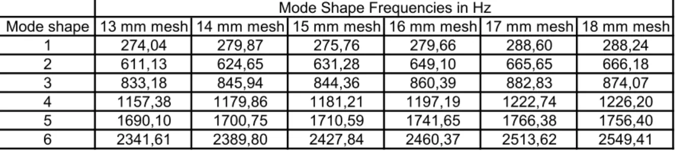
Table 1 (cont.) – Catia model frequencies
Mode shape 13 mm mesh 14 mm mesh 15 mm mesh 16 mm mesh 17 mm mesh 18 mm mesh
1 274,04 279,87 275,76 279,66 288,60 288,24 2 611,13 624,65 631,28 649,10 665,65 666,18 3 833,18 845,94 844,36 860,39 882,83 874,07 4 1157,38 1179,86 1181,21 1197,19 1222,74 1226,20 5 1690,10 1700,75 1710,59 1741,65 1766,38 1756,40 6 2341,61 2389,80 2427,84 2460,37 2513,62 2549,41
Mode Shape Frequencies in Hz
This interval was chosen given that for a mesh unit size lower than 5mm the storage computer capacity needed exceeds the available capacity of the computer used for the tests, and a size of 18mm already leads to results that greatly disagree with the experimental ones. These frequencies give an idea of how the frequencies change when we simply change the type of mesh used in finite element testing. For a better pattern observation, we can display them in a more direct graphic:
Frequency x Mesh Unit Size
0,00 500,00 1000,00 1500,00 2000,00 2500,00 3000,00 0 5 10 15 20
Mesh Unit Size
Fre qu enc y Mode shape 1 Mode shape 2 Mode shape 3 Mode shape 4 Mode shape 5 Mode shape 6
This shows that for the first modes, very little numerical discrepancy is noticed when changing the mesh unit size. But for the later modes, it is expected that this discrepancy rises as high as the mode order is. A further evaluation of the method effectiveness can be done taking into account that discrepancy.
When comparing with the results from the experience [12]: Table 2 – Experimental frequencies
The chosen mesh for our research will be the one with 10mm unit size. For the four first modes, it presents an acceptable percentage discrepancy from the experimental data, plus it is a mesh that is most easily transformed into a square matrix image, which will reduce our efforts in reshaping the finite element data into a bitmap image representation.
Table 3 – Experiment-model percentage frequency difference 10 mm mesh
Mode Shape Difference (%)
1 3,74 2 22,48 3 5,81 4 18,63 5 61,03 6 76,21
It is essential to also remember the finite element test is not susceptible to experimental errors that may occur. So, considering the original data and the final results, the model can be characterized as realistic, and will fit the primary purposes.