Contributions to sparse methods for complex data analysis

HAL Id: tel-02800595

https://hal.inrae.fr/tel-02800595

HAL is a multi-disciplinary open access archive for the deposit and dissemination of sci-entific research documents, whether they are pub-lished or not. The documents may come from teaching and research institutions in France or abroad, or from public or private research centers.

L’archive ouverte pluridisciplinaire HAL, est destinée au dépôt et à la diffusion de documents scientifiques de niveau recherche, publiés ou non, émanant des établissements d’enseignement et de recherche français ou étrangers, des laboratoires publics ou privés.

Distributed under a Creative Commons Attribution - ShareAlike| 4.0 International License

Julien Chiquet

To cite this version:

Julien Chiquet. Contributions to sparse methods for complex data analysis. Life Sciences [q-bio]. Université d’Évry-Val-d’Essonne, 2015. �tel-02800595�

Habilitation à diriger les recherches

présentée par

Julien Chiquet

Contributions to Sparse Methods

for Complex Data Analysis

Présentée et soutenue publiquement le 8 décembre 2015 devant le jury composé de: M. Alexandre D’ASPREMONT École Normale Supérieure (Rapporteur)

M. Arnak DALALYAN ENSAE/ CREST (Rapporteur)

M. Jean-Philippe VERT Mines ParisTech/ Institut Curie (Rapporteur) M Christophe AMBROISE Université d’Évry Val d’Essonne (Examinateur)

Mme _{Florence D’ALCHÉ-BUC Télécom ParisTech (Examinatrice)}

M. Avner BAR-HEN Université Paris 5 (Examinateur)

‘‘Oh, I’m not a percussionist, I just like to hit things.’’

Tom Waits

I

My main background is in appliedmathematics: I graduated from the Université de Technologie de Compiègnein 2003. There, I obtained a degree in computer engineering with a specialty in data mining and an MSc. in computational science. My educational background hence provided me with basics in statistical learning, mathematical mod-eling and numerical analysis.

From 2003 to 2007 came my first years as a novice researcher. They dealt with themes that I will not cover in this document since I consider that my PhD (obtained in 2007) and the associated scientific production do a reasonable job of summarizing this activity. Let me be a little more specific though: this time period corresponds to my MSc. internship and my PhD thesis, during which I worked under the supervision of Nikolaos LIMNIOS. Nikolaos is an expert in stochastic processes – especially of the semi-Markov kind. During this period, I acquired a reasonable understanding of Markov chains and processes, which are a fundamental toolbox in applied mathemat-ics and statistmathemat-ics. I made some contributions in probabilistic modeling and developed skills linked to the implementation of such methods. I also acquired skills for answer-ing research questions with strong practical interests. Above all, I developed a taste for projects with multidisciplinary aspects. This continued during my MSc. internship, I worked at Gaz de France Research and Innovation(GDF) to develop models based upon heterogeneous Markov chains to predict daily temperatures throughout the year in order to optimize pipelines for natural gas transportation (see my MSc. thesis [TS2]). This was also the first time that I encountered a computer language and environment that I found rather weird at this time as a student freshly graduated from computer science school: I was asked by my GDF supervisor Karine V ERNIER to translate all

myMatlab code into an R-package for a more convenient use by GDF’s statisticians.

Taking the Rpath probably led my potential developer career to a dead-end... yet I guess it was for me a new start regarding my approach to modeling, where everything starts from the data themselves. I then continued on the same themes during my PhD [TS1] supported by the French Nuclear Agency (CEA). The point was to develop a stochastic approach to describe the level of degradation of a structure operating in a possibly hazardous environment across time. The random evolution of this so-called degradation process was described by a differential system with a (semi)-Markovian

methods in two journal papers [JP10, JP14]; then, we developed in [JP12] a numerical method to compute the exact reliability function associated with our framework, while another paper dealt mostly with an application in structural reliability [JP13], namely the modeling of fatigue-crack propagation; two book chapters, one summariz-ing the whole PhD work [BC3], and another extendsummariz-ing the model to semi-Markovian fluctuations [BC2] were published.

The second part of my career began when I started to look for an academic position in 2007: the research covered in this manuscript goes from this point to the present.

Immediately after my PhD defense during summer 2007, I got a one-year position as a Research and Teaching assistant in Bernard PRUM’s Lab “Statistique et Génome”, at the Université d’Évry-Val-d’Essonne. There I found in genomics an extremely stim-ulating research area: the biological questioning and the nature of the data themselves raise new challenges regarding statistical modeling, not to mention the potential for applications in fields as diverse as agronomy or cancer care. Motivated by the recent craze for network modeling in biology, I started to work on Gaussian graphical models and sparse methods with Christophe A MBROISE and Catherine MATIAS, which was quite a change in terms of research theme. Fortunately, I was reasonably equipped with the appropriate background in statistical learning. More importantly, I was greatly in-troduced to the subject by Christophe and Catherine and their complementary points of view.

After one year, I luckily obtained a tenured position during autumn 2008 as an Assistant Professor in the same lab. I pursued these themes and co-supervised sev-eral MSc. internships and the PhD theses of Camille C HARBONNIER and Jonathan PLASSAISwith Christophe. I also had (and still have) the good fortune to work with Yves GRANDVALET , who shares his experience in statistical learning, regularization and optimization algorithms, the latter being omnipresent in modern computational statistics. I naturally came across a large variety of problems in genomics that could ad-vantageously be tackled with such tools. I thus chose to focus on regularization, sparse methods and related statistical learning techniques.

From late 2012 to autumn 2015, I received an invited position as an INRA 1 re-searcher in Stéphane ROBIN’s Lab, at AgroParisTech. I have further diversified my fields of application to genetics and agronomy by elaborating more involved regular-ized methods to a broader class of problems. I have collaborated with Stéphane and am now co-supervizing David BAKER’s Post-doctorate with Tristan M ARY-HUARD, about regularization methods for genomic selection. I am also working with Marie-Laure MARTIN-MAGNIETTE and Guillem RIGAILL on network inference in plants, and we are co-supervizing Trung H A’s PhD about multivariate method for high-dimensional data. I have also had other very prolific collaboration with Guillem, notably at the occasion of Pierre G UTIERREZ’s MSc. More generally I have forged tight connections with many members of the lab, for both friendly and professional relationships, which will undoubtedly yield interesting work and much fun!

Finally, I would like to say a word about my direct collaborations with biologists,

1_{“Institut National de La recherche Agronomique”, the French Institute for Research in Agronomy}

according to the technology itself. This work is thus a great source of inspiration for more methodological research and remains essential to me. In such a context, I have had fruitful collaborations with Boulos C HALOUB on polyploïd organisms like colza and wheat in the last couple of years: in [JP5, JP4], I helped for the statistical anal-ysis of transcriptomic data to answer questions specific to polyploidy and have been participating in the co-supervision of Smahane C HALABI’s PhD thesis and Edith LE FLOCH’s post-doctoral fellowship.

Manuscript outline. This document is organized around three chapters. The first chapter depicts the motivations for my research orientations and the related methodological choices. I wish to demonstrate that these choices are pragmatic and “data oriented”. The second chapter presents my contributions to GGM and sparse network inference. The third chapter describes my contributions to regularization methods, in an attempt to account for some data features in the manner by which we shape the regularization – or the penalty term – in the models.

Remark.I use a different numbering for reference to my contributions, which are quasi exhaustively listed for completeness in a separate bibliography at the beginning of this document: I hope this will ease the reading.

I also provide an academic Curriculum Vitæ in the appendix. Its main role is to cite every colleague and student I have worked with, to whom a large part of this work is due.

Julien Chiquet, November 27, 2015

Foreword v

Scientific production 1

1 Introduction and Overview 9

1.1 A typology of complex data . . . 11

1.1.1 Genomics data, an archetype for complex data . . . 11

1.1.2 Data characteristics . . . 16

1.2 Recent approaches in statistical learning . . . 18

1.2.1 New challenges in statistical learning . . . 18

1.2.2 Marrying statistics and optimization . . . 24

1.3 Research overview . . . 32

1.3.1 Themes . . . 32

1.3.2 Organization of the manuscript . . . 34

2 Sparse Gaussian Graphical Models for Network Inference 35 2.1 Background . . . 37

2.1.1 Basics on Gaussian graphical models . . . 37

2.1.2 Sparse methods for GGM inference . . . 38

2.2 Contributions . . . 44

2.2.1 Accounting for latent organization of networks . . . 44

2.2.2 Accounting for sample heterogeneity . . . 49

2.2.3 Accounting for time-course data . . . 53

2.2.4 Accounting for multiscale data: multi-attribute GGM . . . 55

2.3 Perspectives . . . 60

3 Structuring Penalties to Account for Complex Data Features 63 3.1 Background . . . 65

3.1.1 Structured regularization with penalized methods . . . 65

3.1.2 Computational consideration . . . 72

3.1.3 Statistical analysis . . . 75

3.2 Contributions . . . 79

3.2.1 The cooperative-Lasso and sign coherent groups . . . 79

3.2.2 Structured regularization for conditional GGM . . . 88

3.2.3 A quadratic view of sparsity . . . 96

3.2.4 Tree reconstruction with fusion penalties . . . 103

3.3 Perspectives . . . 112

Bibliography 115

Curriculum Vitæ 129

P

[PP1] V. Brault, J. Chiquet, and C. Lévy-Leduc, A fast approach for multiple change-point detection in two-dimensional data, biometrika, submitted.

[PP2] J. Chiquet, T. Mary-Huard, and S. Robin, Structured regularization for condi-tional Gaussian graphical models, arXiv preprint.

[PP3] Y. Grandvalet, J. Chiquet, and C. Ambroise, Sparsity by worst-case quadratic penalties., arXiv preprint.

Journal papers

[JP1] C. Bouveyron, J. Chiquet, P. Latouche, and P.-A. Mattei, Combining a re-laxed EM algorithm with Occam’s razor for Bayesian variable selection in high-dimensional regression, Journal of Multivariate Analysis, 2015, to appear.

[JP2] J. Chiquet, P. Gutierrez, and G. Rigaill, Fast tree inference with weighted fusion penalties, Journal of Computational and Graphical Statistics, 2015, to appear. [JP3] T. Picchetti, J. Chiquet, M. Elati, P. Neuvial, R. Nicolle, and E. Birmelé, A

model for gene deregulation detection using expression data, BMC Systems Biol-ogy, 2015, to appear.

[JP4] B. Chaloub, F. Denoeud, S. Liu, S. Parkin, H. Tang, W. X., J. Chiquet,

and 76 more, Early allopolyploid evolution in the post-neolithic Brassica napus oilseed genome, Science, (6199), 2014, URLhttp://www.sciencemag.org/

content/345/6199/950 .

[JP5] H. Chelaifa, V. Chagué, S. Chalabi, I. Mestiri, D. Arnaud, D. Deffains, Y. Lu, H. Belcram, V. Huteau, J. Chiquet, O. Coriton, J. Just, J. Jahier,

and B. Chalhoub, Prevalence of gene expression additivity in genetically sta-ble wheat allohexaploids, New Phytologist, 197(3):pp. 730–736, 2013, URL

http://onlinelibrary.wiley.com/doi/10.1111/nph.12108/full .

[JP6] J. Chiquet, Y. Grandvalet, and C. Charbonnier, Sparsity in sign-coherent groups of variables via the cooperative-lasso, The Annals of Applied Statistics, 6(2):pp. 795–830, 2012, URLhttp://projecteuclid.org/euclid.aoas/

1339419617.

[JP7] J. Chiquet, Y. Grandvalet, and C. Ambroise, Inferring multiple graphical mod-els, Statistics and Computing, 21(4):pp. 537–553, 2011, URLhttp://dx.doi.

org/10.1007/s11222-010-9191-2 .

[JP8] C. Charbonnier, J. Chiquet, and C. Ambroise, Weighted-lasso for structured network inference from time course data, Statistical Applications in Genomics and Molecular Biology, 9, 2010, URL http://www.bepress.com/sagmb/

vol9/iss1/art15 .

[JP9] C. Ambroise, J. Chiquet, and C. Matias, Inferring sparse Gaussian graphical models with latent structure, Electronic Journal of Statistics, 3:pp. 205–238, 2009, URL http://projecteuclid.org/DPubS?service=UI&version=1.

0&verb=Display&handle=euclid.ejs/1238078905 .

[JP10] J. Chiquet, N. Limnios, and M. Eid, Piecewise deterministic Markov processes applied to fatigue crack growth modelling, Journal of Statistical Planning and Inference, 139(5):pp. 1657–1667, 2009, URLhttp://dx.doi.org/10.1016/

j.jspi.2008.05.034 .

[JP11] J. Chiquet, A. Smith, G. Grasseau, C. Matias, and C. Ambroise, SIMoNe: Sta-tistical Inference for MOdular NEtworks, Bioinformatics, 25(3):pp. 417–418, 2009, URLhttp://dx.doi.org/10.1093/bioinformatics/btn637 .

[JP12] J. Chiquet and N. Limnios, A method to compute the transition function of a piecewise deterministic Markov process, Statistics and Probability Let-ters, 78(12):pp. 1397–1403, 2008, URLhttp://dx.doi.org/10.1016/j.

spl.2007.12.016 .

[JP13] J. Chiquet, N. Limnios, and M. Eid, Modelling and estimating stochastic dy-namical systems with Markovian switching, Reliability Engineering and System Safety, 93(12):pp. 1801–1808, 2008, URLhttp://dx.doi.org/10.1016/j.

ress.2008.03.016 .

[JP14] J. Chiquet and N. Limnios, Estimating stochastic dynamical systems driven by a continuous-time jump Markov process, Methodology and Computing in

Ap-plied Probability, 8:pp. 431–447, 2006, URL http://www.springerlink.

com/content/e8736480p20271l3/ .

Book chapters

[BC1] M. Jeanmoungin, C. Charbonnier, M. Guedj, and J. Chiquet,

Probabilis-tic graphical models dedicated to applications in geneProbabilis-tics, genomics and postge-nomics, chap. Network inference in breast cancer with Gaussian

graph-ical models and extensions, 2014, URL http://ukcatalogue.oup.com/

product/9780198709022.do .

[BC2] J. Chiquet and N. Limnios, Stochastic Reliability and Maintenance Model-ing, vol. 9 of Springer Series in Reliability Engineering, chap. Dynamical systems with semi-markovian perturbations and their use in structural re-liability, Springer, 2013, URL http://www.springer.com/engineering/

production+engineering/book/978-1-4471-4970-5 .

[BC3] J. Chiquet and N. Limnios, Mathematical methods in survival analysis, reliability and quality of life, chap. Reliability of stochastic dynamical systems applied to fatigue crack growth modelling, Wiley / ISTE, 2008, URL

http://eu.wiley.com/WileyCDA/WileyTitle/productCd-1848210108,

[BC4] A. Vacher, C. Tamaddoni-Nezhad, S. Kamenova, N. Peyrard, L. Schwaller, J. Julien Chiquet, M. Smith, J. Vallance, Y. Moalic, R. Sabbadin, V. Fievet, B. Jakuschkin, and D. Bohan, Advances in Ecological Research, chap. Learning Ecological Networks from Next-Generation Sequencing Data, to appear.

Popular science

[PS1] J. Chiquet, Statistique et génome: réseaux biologiques, La gazette des mathématiciens, 130:pp. 76–82, 2011, URL http://smf4.emath.fr/en/

Publications/Gazette/2011/130/ .

Technical reports

[R1] J. Chiquet, Pascal : Probabilistic fracture mechanics applied safety computing age-ing lwr, Tech. Rep. SERMA / LCA/ RT/ 05-3459, CEA, 2005.

[R2] J. Chiquet, Équations différentielles stochastiques appliquées à la modélisation de la fatigue des matériaux, Tech. Rep. SERMA / LCA/ RT/ 05-3583, CEA, 2005.

[R3] J. Chiquet, Vers le développement de modèles aléatoires pour le vieillissement des structures : une approche stochastique, Tech. Rep. SERMA / LCA/ RT/ 04-3417,

CEA, 2004.

Thesis

[TS1] J. Chiquet, Modélisation et estimation des processus de dégradation avec appli-cation en fiabilité des structures, Ph.D. thesis, Université de Technologie de

Compiègne, 2007, http: // tel.archives-ouvertes.fr/ tel-00165782.

[TS2] J. Chiquet, Estimation des températures journalières

à l’aide de techniques markoviennes, Master’s

the-sis, Université de Technologie de Compiègne, 2003,

http: // stat.genopole.cnrs.fr / _media/ members/ jchiquet/ rapportdea.pdf.

C

Contributed talks (international)

[CI1] J. Chiquet, P. Gutierrez, and G. Rigaill, Weighted fusion penalties for tree infer-ence and its oracle properties, in Proceedings of the MLCB NIPS’14 workshop, Montréal, 2014.

[CI2] D. Laloé, F. Jaffrezic, J. Chiquet, and M. Gaultier, FLPCA: a fused-Lasso PCA-based approach to identify footprints of selection in differentiated populations from dense to SNP data: applications to human and cattle data, in Proceedings

of the International Biometric Conference, Florence, Italy, 2014.

[CI3] J. Chiquet, T. Mary-Huard, and S. Robin, Multi-trait genomic selection via multivariate regression with structured regularization, in Proceedings of the MLCB NIPS’13 workshop, South Lake Thaoe, 2013, URL http://ai.

[CI4] P. Gutierrez, G. Rigaill, and J. Chiquet, A fast homotopy algorithm for a large class of weighted classification problems, in Proceedings of the MLCB NIPS’13 workshop, South Lake Thaoe, 2013, URL http://ai.stanford.

edu/~saram/mlcb_2013/MLCB13_submission4.pdf .

[CI5] J. Chiquet, Y. Grandvalet, and C. Charbonnier, Sparsity with sign-coherent groups of variables via the cooperative-lasso, in Proceedings of SPARS’11, Ed-inburgh, 2011, URL http://www.see.ed.ac.uk/drupal/sites/default/

files/spars2011/spars11.pdf .

[CI6] J. Corvol, C. Vrignaud, K. Tahiri, F. Cormier, C. Charbonnier, F. Charbonnier-Beaupel, W. Carpentier, A. Patat, E. Mascioli, Y. Chi-quet, J. Grandvalet, C. Ambroise, G. Edan, and E. Zanelli, Gene expression signature in whole blood after treatment with amino acid copolymer pi-2301 in multiple sclerosis, in European Committee for Treatment and Research in

Multiple Sclerosis, 2010.

[CI7] Y. Grandvalet, J. Chiquet, and C. Ambroise, Inferring multiple regulation net-works, in Proceedings of the MLCB NIPS’10 Workshop, Vancouver, 2010. [CI8] J. Chiquet, N. Limnios, and M. Eid, Reliability evaluation of a dynamical

sys-tem in semi-Markovian environment, in Proceedings of IWAP’08, Compiègne, 2008.

[CI9] J. Chiquet, C. Matias, and C. Ambroise, Penalized maximum likelihood ap-proach for sparse Gaussian graphical models with hidden structure, in Proceed-ings of IWAP’08, Compiègne, 2008.

[CI10] J. Chiquet, N. Limnios, and M. Eid, Modelling the reliability of degradation processes through Markov renewal theory, in Proceedings of ESREL’07, Sta-vanger, 2007.

[CI11] J. Chiquet, N. Limnios, and M. Eid, Modeling and estimating stochastic dy-namical systems with Markov switching, in Proceedings of ESREL’06, Estoril, 2006.

Contributed talks (French)

[CN1 ] T. Mary-Huard, J. Chiquet, A. Célisse, and M. Fuchs, Formule exacte pour la validation croisée dans le cadre de la régression “pool-sample”, in actes des 47e journées françaises de statistique, Rennes, 2015.

[CN2 ] P.-A. Mattei, P. Latouche, C. Bouveyron, and J. Chiquet, Une relaxation continue du rasoir d’Occam pour la régression en grande dimension, in actes des 47e_{journées françaises de statistique, Rennes, 2015.}

[CN3 ] J. Chiquet, T. Mary-Huard, and S. Robin, Inférence jointe de la structure de modèles graphiques gaussiens, in actes des 46e_{journées françaises de statistique,}

Rennes, 2014.

[CN4 ] J. Plassais, J. Chiquet, A. Cervino, and C. Ambroise, A comparison of two

statistical methods combining high-throughput data to predict the level of disease activity in patients with rheumatoid arthritis, in JOBIM’12, Rennes, 2012.

[CN5 ] C. Charbonnier, J. Chiquet, and C. Ambroise, Weighted-lasso for structured network inference for time-course data, in JOBIM’10, Montpellier, 2010.

[CN6 ] J. Chiquet, Y. Grandvalet, and C. Ambroise, Inferring multiple graphical structures, in Workshop MODGRAPHII, JOBIM’10, Montpellier, 2010.

[CN7 ] Y. Grandvalet, J. Chiquet, and C. Ambroise, Inférence jointe de la structure de modèles graphiques gaussiens, in actes de CAp’10, Clermont-Ferrand, 2010. [CN8 ] J. Chiquet, C. Charbonnier, and C. Ambroise, SIMoNe : Statistical Inference

for Modular Networks, in Workshop MODGRAPH, JOBIM’09, Nantes, 2009.

[CN9 ] J. Chiquet, N. Limnios, and M. Eid, Processus markoviens de saut dans les équations différentielles stochastiques appliquées à la modélisation de la fatigue des matériaux, in Congrès Français de Mécanique’05, Troyes, 2005.

[CN10 ] J. Chiquet, N. Limnios, T. Yurizin, and M. Eid, Modèle stochastique de taille critique de fissure dans les structures soumises au vieillissement par irradiation, in Congrès Français de Mécanique’05, Troyes, 2005.

Invited talks

[IT1] Sparse Gaussian graphical models for biological network inference, ISI World Statistics Congress, Hong-Kong, 2013.

[IT2] Sparse Gaussian graphical models for biological network inference, StatLearn’13, Bordeaux, 2013.

[IT3] Sparsity with sign-coherent groups of variables via the cooperative-lasso, Statistics and Modeling for Complex Data, Marne-la-Vallée, 2011.

[IT4] Learning the structure of Bayesian networks with application in post-genomics, International Workshop on Bayesian Networks and Applications in

Post-genomics, Paris, 2010.

[IT5] Penalized maximum likelihood approach for sparse Gaussian graphical models with hidden structure, International Workshop on Applied Probability,

Com-piègne, 2008.

[IT6] Reliability evaluation of a dynamical system in semi-Markovian environment, International Workshop on Applied Probability, Compiègne, 2008.

[IT7] Modelling degradation processes through a piecewise deterministic Markov pro-cess, Mathematical Methodologies for Operational Risk, Eindhoven, 2007.

[IT8] Modelling degradation processes through a piecewise deterministic Markov pro-cess with applications to fatigue crack growth, Recent Advances in Stochastic

S

[SW1] J. Chiquet, SPRING: Structured selection of Primordial Relationships IN the General linear model , 2014.

https://r-forge.r-project.org/projects/spring-pkg/ .

This package fits multivariate regression models using sparse conditional Gaussian graphical modeling with Laplacian regularization.

[SW2] P. Gutierrez, G. Rigaill, and J. Chiquet, Fused-Anova , 2013.

https://r-forge.r-project.org/projects/fusedanova/ .

This package adjusts a penalized ANOVA model with Fusion penalities, i.e. a sum of weighted l1-norm on the difference of each coefficient. The fitting procedure is accompanied by a highly efficient cross-validation method. [SW3] J. Chiquet, Quadrupen: Sparsity by Worst-Case Quadratic Penalties ,

2012.

http://cran.r-project.org/web/packages/quadrupen/ .

This package fits classical sparse regression models with efficient active set algorithms by solving quadratic problems. It also provides a few methods for model selection purposes (cross-validation, stability selection).

[SW4] J. Chiquet, Scoop: Sparse Cooperative Regression , 2011.

http://stat.genopole.cnrs.fr/logiciels/scoop .

This R package fits coop-Lasso, group-Lasso and tree-group Lasso variants for linear regression and logistic regression. The cooperative-Lasso (in short, coop-Lasso) may be viewed as a modification of the group-Lasso penalty that promotes sign coherence and that allows zeros within groups.

[SW5] J. Chiquet, G. Grasseau, C. Ambroise, and C. Charbonnier, SIMoNe: Sta-tistical Inference for MOdular NEtworks , 2010.

http://stat.genopole.cnrs.fr/logiciels/simone .

SIMoNe (Statistical Inference for MOdular NEtworks) is an R package which implements the inference of co-regulated networks based on partial correlation coefficients from either steady-state or time-course transcrip-tomic data. This package can deal with samples collected in different exper-imental conditions. In this particular case, multiple related graphs are in-ferred simultaneously. The underlying statistical tools enter the framework of Gaussian graphical models (GGM). Basically, the algorithm searches for a latent clustering of the network to drive the selection of edges through an adaptive l1-penalization of the model likelihood.

[SW6] S. Lèbre and J. Chiquet, G1DBN , 2008.

http://cran.r-project.org/src/contrib/Archive/G1DBN/ .

A package performing Dynamic Bayesian Network inference.

[SW7] J. Chiquet, Crack growth modeling via (semi)-Markovian switching pro-cesses, 2007.

[SW8] J. Chiquet, Estimating daily temperatures with heterogeneous Markov Chains , 2003.

R package for internal use at Gaz de France.

[SW9] J. Chiquet, Modeling the -phage through agent-based programming , 2002.

1

I

NTRODUCTION AND

O

VERVIEW

If your experiment needs statistics, you ought to have done a better experiment.

Ernest Rutherford

Contents

1.1 A typology of complex data . . . 11

1.1.1 Genomics data, an archetype for complex data . . . 11

1.1.2 Data characteristics . . . 16

1.2 Recent approaches in statistical learning . . . 18

1.2.1 New challenges in statistical learning . . . 18

Computational issues. . . 18

Statistical issues. . . 20

Modeling and interpretability issues. . . 23

1.2.2 Marrying statistics and optimization . . . 24

What do we need? . . . 24

Sparsity, regularization and convex optimization . . . 24

Sparse and regularization approaches to account for complex data structure . . . 28

1.3 Research overview . . . 32

1.3.1 Themes . . . 32

1.3.2 Organization of the manuscript . . . 34

T

informally the kind of data statisticians have to deal with in recent application problems. I build on the example of genomics, with which I am familiar, in order to extract the most striking characteristics of modern data that strongly jeopardize the common way of doing statistics. I exhibit important statistical challenges associated with such data and motivate the use of particular tools at the heart of my research preoccupations, which are at the edge of statistics, optimization and machine learning. I then briefly present the main themes of my research and set them in the landscape of the statistical learning community.

1.1 A

It is now a commonplace to emphasize the irrational way data is gathered about any possible aspect of our world. The collected data sets concern both our surrounding en-vironment (such as astrophysics, plant genomics, or telecommunication network) and ourselves (such as customer data, genomics data, social network data, or any “fancy” smart phone apps that collect information about any of our movements), with a grow-ing contribution of personal data. It has been made possible – or caused? – by the advent of digital technologies: increasing computational and storage capacities offered the possibility of measuring new phenomena and storing the associated data in a new manner. We may think of purely digital phenomena, such as flows of information over the Internet or consumer data collected straight from the cash registers. But the new computer capacities also allow room for new technologies of acquisition and measure-ments, such as high-throughput technology in biology. In a way, the digital revolution creates the need for these new technologies of measurement.

In these various contexts, the common motivation for collecting more data – be-yond the “because we can” – is a hope for a better understanding of the underlying processes that rule the observed systems. This hope comes from the strong faith we place in modern statistics to extract relevant information from massive data: by mon-itoring a huge number of features in a given context, we hope for capturing the ones truly related to the process of interest. Based on the old saying “the more data, the better”, we trust statistical learning methods for this task. But the systematic gather-ing of data at large scales in a very exploratory fashion induces data sets with complex structures: growing databases do not necessarily simplify the statistical analysis, as the collected data endow characteristics which are hardly captured by common intuition or by classical statistical methods.

In this section, I want to enumerate the most striking characteristics of modern complex data that induce new challenges in statistical learning. To this end, I rely on the canonical example of genomics. Indeed, data that have arisen in this context are quite diverse and bring together many of the characteristics shared by modern data.

1.1.1 Genomics data, an archetype for complex data

Genomics is the field of genetics that tries to characterize and analyze the structures and the functions of the genome. This recent discipline is quickly evolving thanks to the advent of biotechnologies and high-throughput techniques. Genomics research was ini-tially motivated mainly by some fundamental questioning related to the understanding of the underlying biological processes. Nowadays it is involved in “real world” applica-tions such as public health (with cancer prevention and classification or computer-aided diagnosis) or agronomy (with plant genomics or marker-assisted selection for breeding enhancement) and is thus partially driven by economic stakes. Hence, there are strong expectations for scientific progress based upon genomics analyses, inducing even more data with continuously renewed technologies.

Genomics was primarily concerned with the characterization of DNA sequences – especially the human DNA sequence –. However, once whole genome-sequencing had been made possible and routinely performed for various organisms, the scope of the discipline considerably broadened: structural genomics, studying the three-dimensional representation of proteins encoded by the genomes, has been facilitated. More impor-tantly, access to the full genomic material of an individual allowed the possibility of

going beyond the static characterization of the genome, notably via the emergence of functional genomics: the objective is to study the dynamic of the cell and to under-stand the complex regulations at stake in molecular biology, from gene and RNA tran-scription (the “transcriptome”) to protein translation (the “proteome”). It is also con-cerned by the way this dynamic – especially gene expression – is altered under various conditions (stress, tumor cell, gene duplication, etc.). In turn, research in functional genomics revealed that gene expression may be altered by reversible phenomena like DNA methylation which do not induce modification of the DNA sequence: this is the scope of epigenomics. Another important emerging research area is metagenomics, simultaneously studying genomes of interdependent organisms living in the same en-vironment.

In short, genomics is interested in a growing number of biological features and evolves jointly with the biotechnologies designed to unravel the processes involving these features in the cell. New discoveries raise new questions urging for omics exper-iments based on refined technologies and so on. In this evolving context, there is an increasing number of protocols for acquiring data at various levels of the cell, from next-generation sequencers to a large collection of array-style technologies. The cou-ple of examcou-ples that follow aim to illustrate the range of data sets that the statistician typically has to deal with in genomics.

Example 1.1. Differential gene expression analysis

With transcriptomic experiments, it is possible to evaluate the activity of the genes within a cell by measuring the quantity of mRNA produced, which we call “gene ex-pression”. Next-generation sequencing techniques can be used to measure this activity by counting the sequences of a given size – or short reads – present in a sample at a given time. These reads are then matched to a catalog of known mRNA sequences (called the transcripts) to assess their expression levels. As an example, Figure 1.1 pro-vides the preprocessed output of an mRNA-Seq experiment on colza [JP4] observed in two tissues from the same biological sample, either from the plant leaf or its root: we plot the counts (resp. the negative counts) associated with the 199,047 transcripts in blue for the root (resp. in red for the leaf).

Based on several replicates of such experiments (generally just a couple!), the ques-tion addressed by differential analysis is to determine a set of transcripts the activity of which is different in two tissues, or discriminates one tissue from another.

counts

transcript number

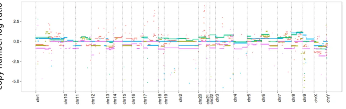
Example 1.2. Detecting genetic aberrations

When a DNA sequence is suspected of being severely altered (as in tumor cells for instance), a major question is to known whether any coding regions have been affected, in which case important functions may be lost in the organism. A quick strategy is to detect gains or losses of regions along the chromosomes by comparing the ploidy level along the sequence between the suspected DNA sample and a reference sample.

To this end, array comparative genomic hybridization (aCGH) measures the copy number variations (CNV) between two genomes at a low resolution. In Figure 1.2, we represent the copy number logarithmic ratio between five DNA samples from breast cancer cell lines and a control sample from the NCI-60 dataset [144]. The signal associ-ated with each cell line is composed of approximately 44,000 points corresponding to ordered features dispatched along the genome. We use a different color for each sample. A statistical question naturally arising is to automatically segment those signals, in order to help find the regions of the genome that are altered. This task can be performed on each single cell line independently or jointly, if those lines share some similarities (here, the kind of cancer of origin).

cop

y

number

log-r

atio

position along the genome

Figure 1.2 – Chromosomal copy number changes (aCGH Agilent 44K Human array)

Example 1.3. Genome-wide association study and marker-assisted selection Small genetic variations between individuals of the same species are common and often without any effect on the phenotype, either because those variations occur on non cod-ing parts of the genome, or because they do not affect the translation process. However, some genetic variants may be associated with some phenotypic alterations in various ways: in plant genomics for instance, these variants are exploited to select lines show-ing the best yields, a field known as marker-assisted selection, or genomic selection. In medical research, association studies are performed to detect variants that induce dif-ferences in a particular disease development, or alter the efficiency of some treatments. These small variations can be assayed at the nucleotide level with SNP (single-nucleotide polymorphism) arrays, that monitor millions of genetic variants at once on predefined loci of the genome. For instance, in the GWAS (Genome-wide association study) presented in [36], SNP-genotyping has been performed on 605 HIV-infected pa-tients in order to evaluate the influence of genetic variants on the disease progression. The latter is measured either by the HIV-DNA level or the HIV-RNA level, the distri-butions of which are represented on the left panel of Figure 1.3a. The objective here is to find a set of features among the 317,000 SNP which jointly explain the response variables measuring the disease progression. The right panel of Figure 1.3a represents a

small block of the empirical correlation matrix of the SNP values in the cohort, which shows interesting patterns that should be taken into account in the statistical modeling.

2 4 6

HIV−DNA level HIV−RNA level

(a) Indicators of disease progression (b) Correlation pattern restricted to the first 200 SNPs

Figure 1.3 – SNP-genotyping (Illumina HapMap300 array) in GWAS

Example 1.4. Regulatory motif discovery

Within the cell, the gene expression is initiated by transcription factors that bind to the DNA upstream from the coding regions, called regulatory regions. This binding occurs when a given factor recognizes a certain (small) sequence called a regulatory motif. As the binding relies on chemical affinity, some degeneracy can be tolerated in the motif definition, and motifs similar but for small variations may share the same functional properties. Hence, genes hosting similar regulatory motifs will be jointly expressed under certain conditions.

In order to detect such regulatory motifs, we aim to relate the expression level of all genes across a series of conditions with the content of their respective regulatory regions in terms of motifs. Figure 1.4 provides insights into the data available to per-form such a task for Plasmodium falciparum, a parasite infamous for causing malaria: on the left panel of Figure 1.4a, we represent gene expression profiling gathered in [19] for the approximately four thousand genes of P. falciparummeasured across 46 con-ditions. A simple hierarchical clustering shows strong patterns both along the genes and the conditions. Concerning the motifs, the data are obtained by counting the oc-currences of a set of candidate motifs in the regulatory regions of each gene (publicy available athttp://plasmodb.org/ ). An example of motif counts data is illustrated on the right panel of Figure 1.4b: we plot the empirical correlation matrix between the motif counts when the set of candidates consists of 4-size motifs composed with the letter fA,C,G,T g and classified by lexicographical order. Strong patterns appear, supporting the assumption that similar motifs have similar effects. The question is then to select motifs showing strong relationships with the expression data. However, for real application purposes, one must consider motifs with a considerably larger size (at least 11), meaning to deal with a huge number of candidates (4 11_).

(a) Clustering of gene expression (row: genes; column: conditions)

(b) Correlation pattern between motifs counts Figure 1.4 – Linking regulatory region sequences to expression data (Affymetrix GeneChip array)

Example 1.5. Gene Regulatory Network Inference

A synthetic view of the regulations at play between a set of genes within the cell is conveniently represented through a graph. The nodes stand for fixed genes while the edges represent interactions due to the genes and their products. The most striking interactions occur between genes encoding for particular proteins, called transcription factors, that are specifically designed in the cell to regulate other genes by binding onto their promoters.

Reconstruction of such networks is extremely informative on the gene expression machinery and has many applications: if one has at one’s disposal a general scheme on how a cell operates in a given condition, we may target a given gene in the network to induce a given behavior at the cell level. In medical research, this could be a better response to a drug treatment. In plant breeding, people may target a gene resulting in a better yield or a better resistance of the plant. Hence, automatic reconstruction – or inference – of gene regulatory networks (GRN) from genomics data has been an important research theme in computational biology. To achieve this task, one would naturally rely on gene expression assays like the ones in Figures 1.1 and 1.4a. However, transcriptomic data is unable to capture the numerous regulations that may operate at various other stages of cell development: complex regulations may occur due to pro-teins binding together; epigenomic phenomena like DNA methylation are known to alter gene expression; and genetic alterations in certain tissues certainly have profound impact on gene expression and regulation. GRN inference is thus a challenging prob-lem, and state-of-the art methods in statistics try to strengthen the inference process by integrating various types of data together and / or by introducing external biological information.

§

These few examples do not claim to provide a comprehensive view of genomics data. Yet, they hopefully illustrate the complexity of their typology, due to differ-ent observation scales, various technologies, continuous / discrete signals, plurality and complexity of the biological processes in place, etc.

1.1.2 Data characteristics

From the statistical point of view, the challenges arising with the analysis of genomics data are mostly the consequences of the following data characteristics.

Large databases. The most obvious feature is the size of the data: as sequencing tech-nologies are widely evolving, the base units in ’omic’ studies are getting smaller, mean-ing larger data-sets to cope with. In the most dreadful cases – typically metagenomics nowadays –, the preprocessed data-sets concern catalogs of transcripts of hundreds of thousands of species weighing several Terabytes. We thus have to deal with samples where the number of features ranges from a few hundred to a few billion.

More variables than individuals. A more challenging and fundamental trait of ge-nomics data is that the sample size remains of the same order as it used to be, while the number of features per sample keeps on increasing with technological improvements. Drawing a sample (like performing a biopsy, growing a plant or breeding an animal) cannot be performed in the same systematic way as many features are measured at once with high-throughput technologies. Thus, statistics are doomed to adapt to the new paradigm of “high-dimensional data”, where the number of variables may exceed the sample size by several orders of magnitude: in the couple of examples depicted above, we typically observe thousands to millions of features to be compared with only dozens to hundreds (sometimes thousands) of individuals.

Multiple sources of heterogeneity. The genomics databases are made up of data sets which are largely heterogeneous. First, we observe diversity in the types of data: in the examples above we encountered continuous variables, counts or categorical data (e.g. from SNP array); moreover some signals are originally available as images or charac-ter strings; we may also think of excharac-ternal biological information encoded as graphs or tree structures. Second, we observe different kinds of dependencies within the data sets depending on the relationships between the features at stake: CNV or SNP data in Examples 1.2 and 1.3 are intrinsically longitudinal because of some spatial relation-ships. Time dependency can also be at stake if a biological process like gene expression levels is measured across the cell cycle. Third, data may live in quite different spaces and at quite different scales due to the fundamental nature of the underlying biological processes, which operate at multiple places and times of the cell, and involving various actors. Many experimental protocols and technologies have been adapted to measure the activity of these biological actors. A consequence is that we have to cope with mul-tiscale data. Last but not least, a larger level of noise can be observed within a given technology, especially the oldest array technique, and incoherence across platforms is likely to occur: transcriptomic experiments can be performed with sequencing tech-nologies as in Example 1.1 or with hybridization arrays as in 1.4. While measuring the same phenomenon, multiple data sets using these two distinct technologies will not share exactly the same features, nor the same precision, nor the same resolution. Highly structured data. The characteristics mentioned up to this point (large data size, high dimensional feature space and heterogeneity) all sound like drawbacks for sta-tistical analysis, which may seem almost hopeless at this stage. Fortunately, genomics data – and most data arising in life science – are deeply structured: hopefully, taking

this structure into account in the statistical modeling may be sufficient to overcome the other difficulties.

This high level of structure has various sources, some being due to the underlying biological mechanisms and the relationships between the biological actors, and some being due to the sampling scheme and the way data-sets are collected. Most of the time however, the structure is only very partially known and must be guessed from the data themselves. The series of examples above illustrates this fact:

In Example 1.1 (differential analysis of mRNAseq colza samples), an obvious structure is due to the tissue where expression is measured (either root or leaf of the plant). With a deeper biological knowledge of the problem, however, one would know that colza is a polyploid organism. This means that some genes called homoeoalleles, sharing very similar sequences, will mostly exhibit highly correlated expression levels. This grouping defines another level of structure in the data.

In Example 1.2 (chromosomal copy number changes in breast cancer), the pre-dictors have a natural spatial structure, that is to say, their ordering along the genome. This structure is intrinsic to the segmentation problem. Another less obvious form of structure arises between the samples: some changes in the ploidy level occur simultaneously in several cell lines (e.g. on chromosome 6), in which case the segmentation would be enhanced if performed jointly.

Example 1.3 (genomic selection for colza) illustrates the existence of a complex pattern of correlation between the genetic markers. This phenomenon is known as linkage disequilibrium in population genetics, which basically states that the allelic status are not independent between two loci. The most obvious reason is due to the spatial organization of the genome: close loci with given allele variants are likely to be jointly inherited. Still, other factors (population structure, mu-tation rate or preferential mating) influence the level of linkage disequilibrium. This explains that the correlation matrix is not defined purely block-wise but through a complex hierarchy.

In Example 1.4 (regulatory motif discovery), a simple heatmap on the gene ex-pression profiles shows a block structure both at the gene and condition levels. Structure on the conditions is likely to be connected with the nature of the con-sidered conditions (heat stress, light stress, cell cycle, etc.). The origin of the gene structure is less clear since it is related to complex direct and / or indirect regulatory relationships between the genes. Finally, a strong correlation pattern arises between the predictors, measured by the occurrence of the motifs in the promoters of all genes. A part of this correlation can be explained by the sim-ilarity between the motifs, when they are equal up to a couple of letters and sorted in the lexicographical order. The correlation that remains may be due to more complex biological features, e.g. a couple of motifs related to a set of genes associated with the same biological pathway.

§

Though motivated by genomics, these characteristics are shared by many complex data sets encountered in application fields beyond biological sciences, like astronomy, imaging, signal processing or finance to cite but a few. The next section shows how these characteristics change our way of doing statistics.

1.2 R

The previous section illustrates how data gathering is deeply evolving and is induc-ing new data characteristics to deal with. An important – though straightforward – remark is to note that most of the traditional goals of statistical learning remain basi-cally unchanged, either in supervised learning (the goal is prediction, via classification or regression) or unsupervised learning (the goal is to unravel interesting patterns via clustering or feature extraction). Indeed, the questions we aim to answer by analyzing modern data sets as in the examples above can be cast as a classical task of statistical learning such as regression, classification, clustering, dimensionality reduction and so on. However, we cannot directly rely on the most favorite and standard methods avail-able since they are not designed to fit data sets with the aforementioned characteristics.

This section starts by showing why traditional approaches are challenged and what their most dramatic limitations towards modern data analysis are. Then, I present the ingredients composing the methods that I develop and work with in my research, designed to answer these challenges. This path follows the recent popular trend in statistical learning which tends to marry tools from statistics and optimization.

1.2.1 New challenges in statistical learning

Various angles are possible to categorize the challenges that jeopardize the traditional way of doing statistics. Hereafter, I successively discuss the computational, the statis-tical and the interpretability issues. This ordering does not reflect the importance of each point; it rather mirrors how they come to the applied statistician’s mind: when dealing with modern data, computational challenges come first, as in the most dramatic cases traditional methods do not even numerically apply. Even when the fit is possible, statistical issues may occur as the assumptions coming with the traditional theoretical guarantees are not fulfilled in this setting. Finally, the fits should be interpreted with caution as standard approaches are not tailored to cope with data heterogeneity nor designed to embed the structure of the problems appropriately.

Meanwhile, an important threat of modern data which connects computational, statistical and interpretability issues together is the problem of high-dimensional fea-ture spaces. In computational biology, the couple of examples given in Section 1.1.1 illustrate that the new standard is to deal with many features p for a moderate sample size n, such that n < p – or even n p–. We commonly speak of a high-dimensional problemwhen analyzing data entering this setting. In many other fields (e.g. signal processing, medical imaging, internet, finance) the new standard is n pwith both n and p large, which corresponds to a class of so-called “big-data” problems. In both situ-ations, one must deal with a large number of features at once, which has many impacts that I shall use as a common thread throughout the statements that follow.

Computational issues.

With the increasing number of features and more generally the advent of large data bases, the computational aspect is now a central question in statistics. First, the al-gorithms used to fit a model must show a rather low complexity regarding the num-ber of features p. This means that many classical methods showing high statistical performance are completely out of reach due to an overly large intrinsic complexity. And second, new statistical methods should be designed to use efficiently the available computer resources (e.g., by allowing parallel computing). However, this latter point

should not overcome the former, in the sense that algorithms with low complexity in pare mandatory in order to deal with high-dimensional feature spaces.

To get better insight on the computational problems at stake, I found it interesting to adopt an optimization point of view. Indeed, most of the statistical methods can be cast as one or a series of optimization problems. Thus, studying the complexity of various classes of problems from the optimization viewpoint undoubtedly provides insights on the limitations of the statistical methods that build on them. To this in-tent, the classification given by Nesterov in [128] is particularly illustrative. It is repro-duced with slight modifications in Table 1.1 that shows the typical operations that we can afford for a given problem size, accompanied with the memory requirement and the range of computational cost (the latter depending on a particular structure of the problem, e.g., sparsity). I added instances from omics that match the various problem scales and the learning tasks typically expected.

class of dimension conceivable computational memory example in expected

problem (# features p ) operations cost requirement omics task

small 100 ₁₀2 _{All p}3 _p4 ₁₀3_{(Kb) – –}

medium 103 ₁₀4 _A 1 _p2 _p3 ₁₀6_{(Mb) transcriptomics network inference}

large 105 ₁₀7 _{Ax p p}2 ₁₀9_{(Gb) association studies variable selection}

huge 108 ₁₀12 _{x+ y log(p) p 10}12_{(Tb) metagenomics clustering}

Table 1.1 – Typical matrix algebra operations with their computational cost and memory

require-ment for various problem scales. A is a pp matrix and x, y are vectors inRp_{(source:[128]).}

Corresponding data regime for some problems in genomics with the desired learning tasks.

This table suggests several comments. First, it gives clues as to the methods that can be applied depending on the situation. Consider for instance the extreme case of metagenomics where one aims to cluster billions of sequences: general agglomera-tive clustering algorithms in O(n3_{) are completely out of reach in this case. It means} that some popular procedures such as UPGMA (Unweighted Pair Group Method with Arithmetic Mean) for average linkage clustering should be banned for some problem scales as it exhibits a quadratic complexity. Second, this table shows that, when possi-ble, we must adapt the optimization procedures used to fit a given statistical method to the problem size. In the case of UPGMA, the method is defined in itself by an algo-rithm and there is no way to change the underlying complexity. In contrast, when a statistical model is adjusted by minimizing for instance a negative log-likelihood, many optimization procedures are available for this purpose. For instance, we may use a second-order method like Newton-Raphson which relies on the first and second derivatives of the log-likelihood. This method converges quadratically to the solution but requires the inversion of a p p matrix at each iteration. Another possibility is to use first order methods, such as the steepest gradient descent method, which only relies on the first derivative of the log-likelihood. Such gradient methods typically have a linear convergence rate, requiring more iterations than Newton’s method to meet the same precision, but only require operations like Ax in Table1.1. Thus, statistical meth-ods originally designed for a medium scale situation can still be applied to larger scale situations1_{if adapting the underlying fitting algorithms is possible: trading some speed} of convergence, meaning more iterations, is the price to pay to scale the dimension by relying on simpler operations at each iteration of the optimization procedure.

1_{Related to this question, Nesterov’s paper [128] reviews subgradient methods for huge-scale problems}

As discussed in the next section, other sources of motivation for using simple and highly-efficient procedures come from the statistical side. Indeed, a major concern in high-dimensional spaces is overfitting, in which case resampling and ensemble methods may be a solution, despite their additional computational cost. This again advocates for highly efficient algorithms designed to use all the computational resources available.

To conclude with this part, the computational aspect turns out to be so important in statistical learning that several authors [15, 90] advocate for criteria that take into account both statistical and numerical performance to compare statistical methods. Statistical issues.

In general, considering large feature spaces is cumbersome since most of our intuition breaks down, especially our geometrical intuition. This is basically due to the fact that the volume of high-dimensional spaces increases exponentially fast compared to the amount of data points available, which are extremely sparse in those spaces. Thus, the sample size n of the data does not have to be smaller than the dimension p for prob-lems to occur. This phenomenon and its various implications are often referred to as the curse of dimensionality. Several illustrations can be found for instance in Chapters 2 and 18 of the classical book [70] of Hastie, Tibshirani and Friedman. In a more recent effort [63], Giraud also gives many instances of this phenomenon that provide inter-esting insights from various points of view (geometrical, probabilistic, statistical and computational). Although I do not aim to investigate exhaustively the numerous man-ifestations of the curse of dimensionality, I underline here two major related problems, namely data scarcityand overfitting.

Data scarcity. In high-dimensional spaces, data points – even when n p– are very isolated and are all at a similar distance from one another: points are so sparsely dis-seminated that the notion of neighborhood is hardly relevant. To illustrate this point, we revisit a small numerical experiment inspired by Figure 1.3 of Giraud’s book [63], which is designed to show that local methods such as local regression or k-nearest-neighbor are doomed to fail in high-dimensional spaces. We consider a random vec-tor X 2 Rp_{with a normal distribution N (0}

p,Ip) and draw a size-n random sample (X1_{,..., X}n_{) with n = 500 and for various values of p 2 f2,10,100,1000g. Elementary} computations show that, for all 1 i < i0 n,

E Xi _Xi0 2

2= 2p, Var X

i _Xi0 2 2= 8p.

As for Giraud in his example with uniform random variables, we also meet in the Gaussian case a pairwise square distance the mean of which grows linearly in p while its standard deviation only grows in p p. Thus, in high-dimensional spaces when p is large, all pairs of points are at a similar distance and thus indistinguishable. Local meth-ods, based upon the notion of neighborhood which is not relevant when pis large, will thus perform poorly. This phenomenon is illustrated on Figure 1.5, where we repre-sent in red the (scaled) histograms of the scaled pairwise distances Xi _Xi0

2= p

2p for all 1 i < i0 _{nand p 2 f2,10,100,1000g.}

At first glance, the most straightforward conclusion drawn from this simple exper-iment – and from other manifestations of the curse of dimensionality – is that separat-ing the noise from the signal looks extremely challengseparat-ing, if not impossible, in high-dimensional spaces. Hopefully, the hypothetical situation where the p features are

density 2 10 100 1000 0.0 0.5 1.0 1.5 2.0

sampling distribution Independent Gaussian Affymetrix xpression array

kX Y k₂=p 2p

Figure 1.5 – Empirical distributions of scaled pairwise distances between vectors inRp

sam-pled fromN (0p,Ip) or from the breast cancer expression data set[67]. Values of p vary in

f2,10,100,1000gto illustrate the concentration of the distance in high-dimensional spaces for the in-dependent Gaussian case. Pairwise distances sampled from expression data are more spread around their mean, meaning more structured data.

independent does not fit the reality and the true underlying space where the data lie is most probably low-dimensional. To support this point, we also report in Figure 1.5 the scaled histograms (in blue) of the scaled distance when X is sampled from the breast can-cer gene expression data studied in [67], where p 44,000 transcripts are monitored for n 500 patients. For random subsets of genes with size p 2 f2,10,100,1000g, the histograms look more spread out than the theoretical one, meaning that we might be able to separate those points according to their pairwise distances. This gives some hope if one has a clue about the shape of the underlying space or of some structure in the data, in other words, if we account for the structure of the problem.

Overfitting. Overfitting affects models which are too complex with low bias but large variance. The consequence is a poor capability for generalization, meaning a large test error. This problem is greatly exacerbated in high-dimensional spaces where distinguishing noise from signal is especially challenging. Moreover, data is so scarce that adjusting a fit with the model that truly generated the observations may lead to poorer results than applying simpler models, with high bias but low variance. Let us consider a simple idealistic example in linear regression to illustrate this point: we draw f(xi, yi)gi= 1,...,nwith xi sampled in the interval [ , ] and we choose the “true” relationship such that yi = sin(2xi) + N (0, 2). We choose to meet a coefficient of determination R2 _{0.8. Now, suppose that we do not know the nature of the true} relationship. We fit the data using polynomial regression with order p, that is

y_i = ₀+ p X

j= 1

This toy example allows us to show on a two-dimensional fit the effect of an excessively complex model with too many features, that is, living in a high-dimensional space. The order p of the polynomial is used to control the dimension p of the feature space, mean-ing the model complexity. We study cases where p 2 f1,...,50g, i.e. models as simple as a regression line and as complex as a polynomial with degree 50. We consider three regimes for the training, with sample size n 2 f10,50,200g. Whenever possible, Model (1.1) is fitted with ordinary least squares (OLS). In cases when n < p, (which occurs only when p > 10 and n = 10), we use ridge regression with a tiny regularization pa-rameter in order to encounter as little bias as possible and thus stick close to an “OLS fit”. Results from this experiment are summarized in Figure 1.6. The three columns correspond to the three possible regimes for the sample size. The first row shows ex-amples of fits with p in f1,5,20g, for a single data set. Data points used for the training set are plotted in plain black, while a set of 1,000 points composing the (unreachable) test set appears shaded black. The second row shows the estimated generalization error with a hundred replications of the experiment conducted in the first row, using the test set for evaluating the generalization error.

n= 10 n= 50 n= 200 model fit (one sho t) ● ● ● ● ● ● ● ● ● ● −2 −1 0 1 2 −2 0 2 p 1 5 20

set _{test training}●

● ● ● ● ● ● ● ● ● ● ● ● ●● ● ● ● ● ● ● ● ● ● ● ● ● ● ● ● ● ● ● ● ● ● ● ● ● ● ● ● ● ● ● ● ● ● ● ● ● −2 −1 0 1 2 −2 0 2 ● ● ● ● ● ● ● ● ●● ● ● ● ● ●● ● ● ● ● ● ● ● ● ● ● ● ● ● ● ● ● ● ● ●● ● ● ● ● ● ● ● ●● ● ● ● ● ● ● ● ● ● ● ● ● ● ● ● ●● ● ● ●● ● ● ● ● ● ● ● ● ● ● ● ● ● ● ● ● ● ● ● ● ●● ●● ● ● ● ● ●● ● ● ●● ● ● ● ● ● ● ● ● ● ● ● ● ● ●● ● ●● ● ●● ● ● ● ● ● ● ● ● ● ● ● ● ● ● ● ● ● ● ● ● ● ● ● ● ● ● ● ● ● ● ● ● ● ● ● ● ● ● ● ● ● ● ● ● ● ● ● ● ● ● ● ● ● ● ● ● ● ●● ● ● ● ● ● ● ● ● ● ● ● ● ● ● ● ● ● ● ● ● −2 −1 0 1 2 −2 0 2 xaxis er ror (log scale) 1e+02 1e+05 1e+08 0 10 20 30 40 50 1e+03 1e+08 1e+13 1e+18 0 10 20 30 40 50 10 1000 0 10 20 30 40 50 model dimension ( p)

Figure 1.6 – Overfitting is especially at play with high-dimensional data.

What conclusion can be drawn from this experiment? First, we obviously do not need to be in the n < p setup to overfit: considering large feature spaces is enough. Second, we see that this phenomenon is exacerbated when n gets smaller compared to p. More precisely, consider the case when n = 10: from the estimated test error (bot-tom left), the model which generalizes the best is the simple regression line, which is far from the one that truly generates the data (see the test set in the first row, showing a sinusoidal relationship). But there are so few data points that models lying in feature spaces with moderate dimension (e.g. p = 5) – thus close to the true underlying gen-erative model – already overfit and show large variance, causing a poor generalization.

This example supports the use of simple models, with potentially high bias but well controlled variance, as they seem to be sufficient to capture the main tendency of data sets that lie in high-dimensional feature spaces.

Modeling and interpretability issues.

The vast number of features is again at play regarding the modeling side of statistics, and consequently the way we interpret the fits. Typically, models involving many or ill-assorted features conflict strongly with our common sense; even if they show good predictive performance or summarize the data well, there are many application fields, notably in genomics and biology, where the interpretation of the fitted model is as important as its performance. In supervised problems, the features sought are those having a strong relationship (ideally causal) with the target response. In unsupervised problems, the objective is to unravel the underlying structure between the features themselves, which structure rules the observed system. To this end, the statistician should rely on the tools available in statistical learning for feature selection or feature extraction, the utility of which becomes even more important when the number of features grows. But again, traditional tools have to be rethought since they are not always calibrated to extract relevant information from data that live in large spaces.

To support this statement, we bring together the observations made on our two preceding numerical experiments: in Figure 1.5, we assess that, in most computational biology experiments, the dimension of the feature space that rules the underlying pro-cess is much lower than the number of features considered. The question is thus to find this underlying space, which may be done by means of feature selection or feature extraction techniques. However, in high-dimensional problems, the model which is the closest to the generative model – or to the biological process underneath – might not be the one that generalizes the best, due to the scarcity of data. This has been il-lustrated in Figure 1.6, where the straight line shows the smallest generalization error but is far from the true underlying model. Hence, one must be extremely careful when interpreting models fitted in a high-dimensional setup. This should especially be kept in mind in genomics where we often deal with medical data and where the temptation to interpret the inferred relationships as causal is huge.

A possible way to remedy the risk of incorrect interpretation is to adapt feature selection and extraction methods to only explore subspaces that are plausible according to the underlying biological process. In other words, we should add some constraints to the models by means of structural information that expresses our prior knowledge. This remark advocates for using statistical models that impose special structures on the features. Indeed, structure integration in the model should lead to more interpretable models, which is mandatory when dealing with millions of features.

§

This part has provided insights on the limitations of the traditional methods to-wards analyzing modern complex data. We thus hopefully have a good idea of the requirements of modern statistical methods. The next section basically justifies the general strategy constituting the backbone of all the research works presented in this thesis, in an effort to provide the community with methods fulfilling these require-ments.

1.2.2 Marrying statistics and optimization

This section starts by summarizing the most desirable requirements of modern statis-tical methods regarding the challenges discussed so far. Then, I describe how, by bring-ing together tools from statistics and optimization, efficient strategies have emerged to tackle these challenges. In particular, I detail a typical strategy involving regularization and convex sparse methods, which are a central building block of my contributions. What do we need?

Regarding the computational, statistical and interpretability issues mentioned in Sec-tion 1.2.1, an ideal method would be one fulfilling the following principles, which apply whatever the learning task (regression, classification, clustering).

1. Favor simple models.The use of simple models is mandatory in order to avoid overfitting, especially at stake in high-dimensional spaces. In other words, we should ban overly complex models which generalize badly when data is scarce, or at least strongly control their variance. Moreover, the use of simple models typically limits the computational burden.

2. Favor models involving interpretable structures.Models fitted in high-dimensional spaces should be cautiously interpreted. A possible way to limit the risk of bad interpretations is to rely on statistical models involving strong relationships be-tween the variables, with easily absorbed representations (such as hierarchies, orderings or conditional dependencies).

3. Perform dimension reduction.Even when using simple models and interpretable structures of representation, the number of variables associated with the many features at hand should be controlled. Hence, we look for methods that reduce the original feature space, by performing feature extraction or feature selection jointly with the original task (prediction, classification or clustering). On top of favoring interpretability, this also controls the complexity of the models. 4. Account for prior knowledge.The methods should be flexible enough to allow the

integration of prior information related to the underlying feature space. Hence, by biasing the feature extraction or selection processes, we hope to enhance both the interpretability of the model and the predictive performance.

5. Favor algorithms with low/ controllable complexity.The algorithms must show a

globally low complexity regarding the dimension of the feature space. On top of this, we should favor methods the optimization of which can adapt to the prob-lem size, achieving a tradeoff between accuracy and complexity that depends on the problem dimension (see Section 1.2.1).

Sparsity, regularization and convex optimization

In order to develop procedures that meet these prerequisites, popular methods have recently emerged in closely related fields such as statistics, machine learning and com-press sensing. They all aim at revisiting standard statistical approaches from the angle of optimization, by changing the original problem from this renewed point of view. Let us attempt an outline of the strategy commonly followed by these proposals: