A Lagrangian study of inhomogeneous turbulence

(1)

HAL Id: tel-01739689

https://tel.archives-ouvertes.fr/tel-01739689

Submitted on 21 Mar 2018

HAL is a multi-disciplinary open access archive for the deposit and dissemination of sci-entific research documents, whether they are pub-lished or not. The documents may come from teaching and research institutions in France or abroad, or from public or private research centers.

L’archive ouverte pluridisciplinaire HAL, est destinée au dépôt et à la diffusion de documents scientifiques de niveau recherche, publiés ou non, émanant des établissements d’enseignement et de recherche français ou étrangers, des laboratoires publics ou privés.

A Lagrangian study of inhomogeneous turbulence

Nickolas Stelzenmuller

To cite this version:

Nickolas Stelzenmuller. A Lagrangian study of inhomogeneous turbulence. Fluids mechanics [physics.class-ph]. Université Grenoble Alpes, 2017. English. �NNT : 2017GREAI109�. �tel-01739689�

(2)

THÈSE

pour obtenir le grade de

DOCTEUR DE LA COMMUNAUTE

UNIVER-SITÉ DE GRENOBLE-ALPES

Spécialité:

Mecanique des Fluides, Procedes, Energetique

Arrêté ministériel : 25 mai 2016

Présentée par

Nickolas S

TELZENMULLER

Thèse dirigée par:

M. Nicolas MORDANT, PROFESSEUR

UNIVERSITÉ DEGRENOBLE-ALPES

preparée au sien du

Laboratoire des Ecoulements Géophysiques et Industriels École doctorale: IMEP-2

Étude Lagrangienne d’une turbulence

inhomogène

Thèse soutenue publiquement le 20 octobre, 2017 devant le jury composé de:

M. Emmanuel LÉVÊQUE, Rapporteur

Directeur de recherche , LMFA, École Centrale de Lyon

M. Nicholas T. OUELLETTE, Rapporteur

Associate Professor, Stanford University M. Alain CARTELLIER,

Directeur de recherche, LEGI, Université de Grenoble-Alpes Mme. Anne TANIÈRE,

Professeur, LEMTA, Université de Lorraine Presidente de jury

M. Romain VOLK,

(3)

A Lagrangian study of inhomogeneous turbulence

Abtstract: Inhomogeneous turbulence is experimentally investigated in a Lagrangian framework. Measurements of tracer and non-tracer particles in a turbulent channel were made, and were used to extract Lagrangian statistics conditioned on their initial distance to the channel wall. Highly resolved in time and space, these measurements provide the three components of position, velocity, and acceleration along a particle trajectory from very close to the channel wall (y+≈ 10) to the channel center. Lagrangian time correlations allow the direct measurement of velocity and acceleration timescales in each direction, and characterize the inhomogeneity and anisotropy of the turbulent channel from the Lagrangian perspective. Small scale-anisotropy, characterized by the skewness and the correlation of the components of the acceleration, was found to be significant throughout the channel. Significant scale separation between the magnitude and com-ponents of acceleration was found across the channel, even in the near-wall region. Two classes of non-tracer particle trajectories were also measured, allowing direct comparison of tracer and non-tracer statistics from the highly-sheared anisotropic zone near the chan-nel wall to the more homogeneous outer layer. Non-tracer acceleration statistics in the turbulent channel were found to be significantly different from similar results in homoge-neous, isotropic turbulence. These statistics are necessary components of advanced La-grangian stochastic models to predict dispersion and mixing in inhomogeneous turbulence. Keywords: Turbulence, Lagrangian, Turbulent Channel, 3-D PTV

Résumé: Une turbulence inhomogène est étudiée expérimentalement dans un contexte lagrangien. La mesure des trajectoires de traceurs lagrangiens et de particules inertielles a été effectuée dans un canal plan turbulent et a été utilisée pour obtenir des statistiques lagrangiennes conditionnées à leur distance initiale par rapport à la paroi. Ces mesures à haute résolution en temps et en espace fournissent les trois composantes de la posi-tion, la vitesse et l’accélération le long de la trajectoire d’une particule individuelle depuis des distances très proches de la paroi ( 10 unités de paroi) jusqu’au centre du canal. Les corrélations temporelles lagrangiennes ont permis la mesure directe des échelles de temps de la vitesse et l’accélération dans chacune des trois directions. Ces échelles caractérisent l’inhomogénéité et l’anisotropie du canal turbulent dans une perspective lagrangienne. Une anisotropie à petite échelle, quantifiée par la "skewness", et les cor-rélations entre composantes de l’accélération sont observées dans tout le canal. Une séparation d’échelle significative entre les composantes de l’accélération et son amplitude a été mesurée au travers du canal notamment dans la zone proche de la paroi. Deux classes de particules inertielles ont été étudiées permettant ainsi la comparaison directe entre statistiques des traceurs et des non-traceurs dans la zone de fort cisaillement et de forte anisotropie proche de la paroi jusqu’à la région plus homogène du centre. Les propriétés statistiques des particules inertielles dans le canal turbulent sont significa-tivement différentes de celles observées en turbulence homogène isotrope. Ces statis-tiques sont les ingrédients nécessaires à la construction de modèles stochasstatis-tiques la-grangiens pour la prédiction de la dispersion et du mélange en turbulence inhomogène. Mots-clés: Turbulence, Lagrangien, Canal turbulent, 3-D PTV

(4)

Acknowledgments

When I arrived at LEGI to start my PhD I spoke no French, but was determined to learn. As I began setting up the experiment, my fumbling attempts at communication led to a series of comical sketches, in which the long suffering technicians and staff were subjected to my extremely bad French supplemented with gestures. The humor, patience, and generosity with which I was received was remarkable, and will remain a fond memory for a long time to come.

In addition to their warm welcome, the technical expertise of Laure Vignal, Joseph Virone, Mile Kusulja, Gaby Moreau, Samuel Viboud, and Jean-Paul Thibault was invaluable to the success of the experiments.

Nicolas Mordant and I spent many an agreeable hour puzzling over the often counter-intuitive Lagrangian properties of turbulence. In my moments of self-doubt and discour-agement(of which there were a few), his evident intellectual curiosity and enthusiasm for our subject were very encouraging.

I would like to thank the co-authors of the article that appears in this thesis, especially Juan Ignacio Polanco and Ivana Vinkovic, for their permission to include the article. It was a real pleasure to discuss and collaborate with them on this project.

Special thanks to Philippe Marmottant and Nicolas Plihon for the gracious loan of their high-speed cameras, without which these experiments would not have been possible.

Many thanks to the members of the thesis committee, especially the referees Emmanuel Lévêque and Nicholas Ouellette. Their time, insightful comments, and kind words at the thesis defense were very much appreciated.

My colleagues at LEGI, many of whom became close friends, provided discussion, a helping hand, technical support, and encouragement. The solidarity and conviviality I found among the PhD students and post-docs was a joy.

Finally, I would like to thank my partner Steph for her acceptance of my long nights at the lab, her encouragement when I was discouraged, and especially her unflagging faith in me.

(5)

(6)

List of figures

1.1 Reynolds’ turbulence transition experiment . . . 4

1.2 Schematic view of the Kolmogorov scaling of velocity autocorrelation . . . . 10

1.3 The PDF of velocity increment reproduced from Mordant et al[1] . . . 10

1.4 Schematic of a turbulent channel . . . 14

1.5 Profiles of velocity in the turbulent channel . . . 17

1.6 Sketch of a horseshoe vortex, reproduced from Adrian[2] . . . 18

1.7 C∗₀as a function of Reynolds number in DNS of isotropic turbulence . . . . 22

2.1 Selected tracer particle trajectories in the near-wall of a turbulent channel . 31 2.2 Sketch of the turbulent channel used in the experiment . . . 33

2.3 CAD rendering of water tunnel . . . 37

2.4 Tranquilization chamber. . . 38

2.5 Excitation and emission spectra of tracer particles . . . 40

2.6 Schematic view of the PTV system . . . 43

2.7 Particle images examples . . . 45

2.8 Histogram of pixel intensities . . . 46

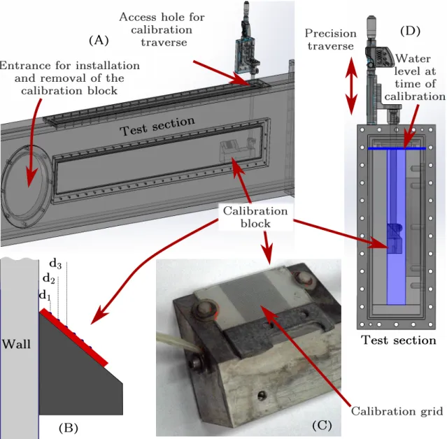
2.9 The calibration block shown in the test section . . . 48

2.10 Schematic of the 3-D stereo-matching. . . 51

2.11 Particle tracking algorithm . . . 52

2.12 Track reconnection example . . . 54

2.13 Schematic of the reconnection algorithm. . . 55

2.14 Data processing schematic . . . 57

2.15 Trajectory data structures . . . 58

2.16 Gaussian kernel frequency response . . . 59

2.17 Continuous and discrete Gaussian kernels . . . 60

2.18 An example of smoothed derivative calculations. . . 61

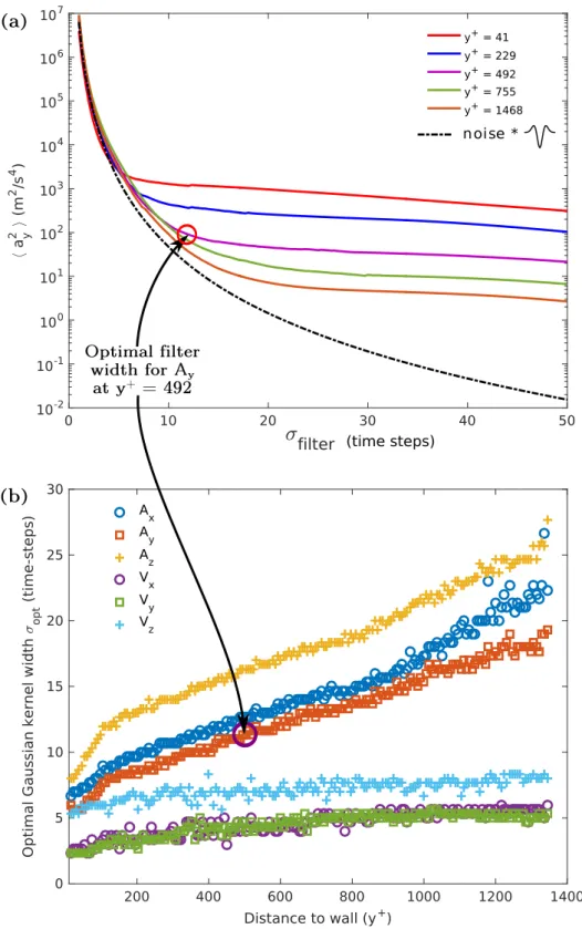
2.19 Acceleration variance as a function of filter width . . . 62

2.20 Example of error in a single trajectory . . . 64

2.21 Particle finding error analysis example . . . 66

2.22 Particle finding error in the finding of synthetic particles . . . 67

2.23 The normalized autocorrelation of the acceleration of delta-correlated noise for various filter width . . . 68

2.24 Illustration of statistical bias due to the finite measurement volume.. . . 69

2.25 DNS domain . . . 71

3.1 Uncorrected mean velocity profile, with selected histograms . . . 75

3.2 Mean streamwise velocity profile with velocity magnitude correction . . . . 76

3.3 Eulerian velocity variance across the channel . . . 77

3.4 Reynolds stress across the channel . . . 78

(9)

3.6 Skewness and flatness of the components of velocity . . . 81

3.7 Conditional means of the fluctuating velocity components . . . 82

3.8 Mean acceleration and acceleration variance profiles. . . 84

3.9 PDFs of the components of acceleration . . . 86

3.10 Joint PDFs of the components of acceleration at four distances from the wall. 87 3.11 Skewness and flatness of the acceleration components across the channel . 88 3.12 The mean correlation of acceleration components across the channel . . . . 90

3.14 The absolute values of the parallel and perpendicular components of accel-eration, projected on the ˆx, ˆy, and ˆz unit vectors. . . . 93

3.15 Definition of the longitudinal (φ) and wall-normal (θ) angles; figure adapted from Zamansky et al [3]. . . 93

3.16 PDF of the wall-normal (θ) orientation of acceleration at various distances from the wall . . . 94

3.17 PDF of the longitudinal (φ) orientation of acceleration at various distances from the wall . . . 95

3.18 Variances of the sine of the longitudinal (φ) and wall-normal (θ) angles, normalized by the variance in the isotropic case . . . 96

3.19 The mean of A · V across the channel. . . 97

3.20 Mean Lagrangian power across the channel, and the individual components of equation 3.27 . . . 99

4.1 Illustration of trajectory binning . . . 104

4.2 Lagrangian mean wall-normal position for two different binning strategies. 105 4.3 Number of tracer particle trajectories of lengthτ+. . . 106

4.4 Mean Lagrangian velocities at three locations, with estimates at smallτ . . . 109

4.5 Mean difference between Lagrangian and Eulerian streamwise velocity at three locations in the channel. . . 110

4.6 Mean Lagrangian wall-normal positions and wall-normal velocities . . . 111

4.7 Illustration of the limits of the model shown in equation 4.32.. . . 112

4.8 Mean square dispersion in the wall-normal direction from six locations in the channel. . . 113

4.9 Normalized mean square dispersion in the wall-normal direction . . . 114

4.10 Rate of dispersion in the wall-normal direction for six locations in the channel.115 4.11 Time-evolution of the PDFs of wall-normal position in buffer layer . . . 116

4.12 Time-evolution of the PDFs of wall-normal position in log layer . . . 117

4.13 Sample high-acceleration particle tracks obtained from DNS . . . 121

4.14 Sketch of the turbulent channel used in the experiment . . . 122

4.15 Mean and variance velocity profiles . . . 123

4.16 Mean and variance acceleration profiles . . . 124

4.17 Illustration of the Lagrangian averaging procedure . . . 125

4.18 Lagrangian auto-correlations of streamwise (ρxx), wall-normal (ρy y) and spanwise (ρzz) particle acceleration . . . 126

4.19 Lagrangian auto-correlation of acceleration magnitude and acceleration cross-correlations . . . 126

4.20 Lagrangian correlation between streamwise and wall-normal acceleration components . . . 127

4.21 An example of how Lagrangian velocity time scales are calculated . . . 129

(10)

4.23 Lagrangian acceleration time scales normalized by the local Kolmogorov

timescale (DNS results only) . . . 130

4.24 Lagrangian time scale ratios. . . 130

4.25 PDF of streamwise, wall-normal and spanwise particle acceleration . . . 133

4.26 Skewness of streamwise and wall-normal acceleration components . . . 133

4.27 Joint PDF of streamwise and wall-normal acceleration at y+= 15 and 59 . . 134

5.1 Normalized acceleration variance of large neutrally-buoyant particles (repro-duced from [4]) . . . 141

5.2 Schematic of the experimental setup used for the measurements of the heavy and large neutrally-buoyant particles . . . 142

5.3 Particle characteristics across the channel . . . 145

5.4 Mean velocity gradient at the particle scale . . . 147

5.5 Acceleration variance as a function of filter width for the three classes of particles . . . 148

5.6 Example of the choice of an optimal acceleration filter for the non-tracer particles . . . 150

5.7 Acceleration variance for the three classes of particle . . . 151

5.8 Acceleration rms ratios for three particle classes . . . 152

5.9 a0for tracer and large neutrally-buoyant particles. . . 153

5.10 Normalized acceleration variance of the heavy particles in the channel plot-ted against the local Stokes number . . . 154

5.11 Covariance of acceleration for the three classes of particles. . . 155

5.12 Autocorrelation of acceleration for the three types of particles in the near-wall region . . . 158

5.13 Autocorrelation of acceleration for the three types of particles in the outer layer159 5.14 Cross-correlation of acceleration for the three types of particles . . . 160

5.15 Acceleration timescales for the three types of particles . . . 161

5.16 Ratio between the particle and fluid acceleration timescales . . . 162

A.1 Lagrangian autocorrelations of acceleration for the streamwise (x), wall-normal (y), and spanwise (z) components of acceleration. . . II

A.2 Lagrangian autocorrelations of velocity for the streamwise (x), wall-normal (y), and spanwise (z) components of velocity. . . III

A.3 Lagrangian correlations of the streamwise and wall-normal components of acceleration. . . IV

A.4 Lagrangian correlations of the streamwise and wall-normal components of velocity. . . V

A.5 Lagrangian cross-correlations of acceleration and velocity (same component) VI

A.6 Lagrangian cross-correlations of acceleration and velocity (different compo-nent) . . . VII

A.7 Non-normalized autocorrelations of acceleration (〈ai(0)ai(τ)〉) for the three

classes of particle. The autocorrelations are calculated from trajectories that are in the bin y+= 0 − 37.5 at t = 0. . . . IX

classes of particle. The autocorrelations are calculated from trajectories that are in the bin y+= 37.5 − 75 at t = 0. . . . X

classes of particle. The autocorrelations are calculated from trajectories that are in the bin y+= 75 − 150 at t = 0. . . . XI

(11)

classes of particle. The autocorrelations are calculated from trajectories that are in the bin y+= 150 − 225 at t = 0. . . . XII

classes of particle. The autocorrelations are calculated from trajectories that are in the bin y+= 225 − 300 at t = 0. . . . XIII

classes of particle. The autocorrelations are calculated from trajectories that are in the bin y+= 300 − 375 at t = 0. . . . XIV

classes of particle. The autocorrelations are calculated from trajectories that are in the bin y+= 375 − 450 at t = 0. . . . XV

classes of particle. The autocorrelations are calculated from trajectories that are in the bin y+= 450 − 525 at t = 0. . . . XVI

classes of particle. The autocorrelations are calculated from trajectories that are in the bin y+= 525 − 600 at t = 0. . . . XVII

classes of particle. The autocorrelations are calculated from trajectories that

(12)

List of Tables

2.1 Design parameters in PTV system . . . 42

2.2 Key parameter affecting ease of particle tracking . . . 53

2.3 Tracer particle raw dataset description . . . 56

2.4 Scaling variables mean and uncertainty . . . 64

(13)

(14)

Motivation

Our eyes are instinctively drawn to motion. Watching snowflakes in a storm, dust caught in a ray of sunlight, or leaves on the surface of a river can be almost hypnotic. This is turbulence as understood by children—following a bubble as it dances in the air. This intu-itive view of turbulence is formalized by Lagrangian kinematics, which follows a particle trajectory in time.

The study of turbulence in a Lagrangian framework is not new: G. I. Taylor formulated a theory of the dispersion of particles in turbulence using a Lagrangian framework in 1921, and more sophisticated Lagrangian models for dispersion have been developed since. Nevertheless it is only in the last 20 years, with the development of new measur-ing technologies and increased computmeasur-ing power, that we have able to directly observe small particles in turbulence at high resolution. Measuring particle trajectories over time allows us to observe how the position, velocity, and acceleration evolve along the particle trajectory—how the particle experiences the turbulence. Statistics formed from these measurements provide a Lagrangian statistical description of turbulence. For example, statistics of the velocity along the trajectory at two times separated by a time-lag may be measured, e. g.

v(t ) − v(t +∆t ) (1)

The shape of the probability density function of this Lagrangian velocity increment is approximately Gaussian for large∆t , but is increasingly non-Gaussian as∆t is decreased. For very small values of∆t the velocity increment is closely related to the acceleration:

a ≡ lim

∆t →0

v(t +∆t ) − v(t)

∆t (2)

which is a strongly intermittent quantity: accelerations up to 50 times the root-mean-square acceleration have been measured experimental. Statistics in the time-correlations of velocity and acceleration, for example

a(t +∆t )a(t )

〈a2〉 (3)

also provide a useful Lagrangian description of turbulence. The velocity decorrelates relatively slowly, and is directly related to the dispersion of fluid particles from a point-source in turbulence. Acceleration decorrelates rapidly, although the correlation of the magnitude of acceleration decays quite slowly in comparison.

Models of varying complexity have been proposed to explain and/or predict these observations. For example, multifractal models formulated in a Lagrangian framework have been used to predict the increasingly non-Gaussian distributions of the velocity increment, and of acceleration. Stochastic dispersion models use time-correlations of velocity and acceleration to recreate fluid particle trajectories. Multifractal random walk, and acceleration-orientation random walk models predict the rapid decorrelation of accel-eration and the slow decorrelation of the magnitude of accelaccel-eration.

(15)

The vast majority of Lagrangian experiments, simulations, and models have focused on homogeneous isotropic turbulence (HIT). The symmetries of high-Reynolds number, homogeneous, isotropic turbulence create a simplified academic framework in which to study turbulence. Models developed in this framework may then be adapted, with varying degrees of success, to the more complicated, realistic cases of lower-Reynolds number, inhomogeneous, anisotropic turbulence. In order to adapt models developed in HIT to more realistic contexts, we must first understand how inhomogeneous turbulence differs from HIT. Inhomogeneous turbulence has long been studied from a practical perspective, as many engineering applications involve wall-bounded turbulence. Almost all of this work has considered inhomogeneous turbulence in an Eulerian framework. From the Lagrangian perspective we know very little about inhomogeneous turbulence. There are many open questions, e. g. in a wall-bounded turbulent flow, how do Lagrangian statistics change with distance to the wall? At what distance to the wall is statistical isotropy reestablished? Are Lagrangian statistics more or less susceptible to the large scale inhomogeneity than Eulerian statistics?

In addition to the behavior of the fluid turbulence, behavior of non-tracer particles in turbulence is also of considerable interest. A wide range of practical applications are concerned with how particles interact with turbulence. Non-tracer particles diverge from fluid particle trajectories, but where and how this divergence occurs is not fully known. Models and mechanisms have been proposed for some classes of particles, e. g. very small, heavy particles, but again, almost all of our understanding relates to particle dynamics in homogeneous isotropic turbulence.

This thesis attempts to respond to these gaps in our knowledge. We use the instruments and techniques developed in the last 20 years of high-resolution Lagrangian measurements and apply them to a turbulent channel flow. The turbulent channel flow in which these measurements were taken is a stationary, moderate-Reynolds number turbulent flow with a single direction of inhomogeneity. This relatively simple configuration allows the measurement of Lagrangian statistics from the highly sheared, strongly anisotropic near-wall region to the quasi-homogeneous center of the channel. Tracer particle measurements allow the extraction of Lagrangian statistics of the fluid turbulence. Two classes of non-tracer particles were also measured, allowing us to explore the effects of inhomogeneity on non-tracer particle statistics.

This thesis is organized as follows. Chapter1introduces fundamental concepts in turbulence, provides an overview of previous Lagrangian investigations in homogeneous turbulence, briefly outlines turbulent channel flow, and gives a survey of Lagrangian stochastic modeling. The experimental details are given in chapter2, which also provides a discussion of the design and constraints involved in such measurements. Eulerian tracer particle results in the turbulent channel are presented in chapter3, with a focus on the one-time statistics of acceleration across the turbulent channel. Chapter4presents Lagrangian results in position, velocity, and acceleration for tracer particles. Finally, non-tracer particles are considered in chapter5.

(16)

Chapter 1 Introduction and Theory

1.4 Lagrangian statistics in inhomogeneous turbulence . . . . 27 Moreover, I soon understood that there was little hope of developing a pure, closed theory, and because of the absence of such a theory the investigation must be based on hypotheses obtained in processing experimental data A. N. Kolmogorov

(17)

1.1 Fluid turbulence from a Lagrangian point of view

1.1.1 What is turbulence?

The dynamics of incompressible Newtonian fluids are given by the deceptively simple equations for the conservation of fluid mass

∂Ui ∂xi = 0 (1.1) and momentum DUi Dt = − 1 ρ ∂P ∂xi + ν ∂2Ui ∂xj∂xj (1.2) whereρ and ν are the fluid material properties of density and kinematic viscosity, respec-tively (taken here to be constant), and U and P are the dynamical quantities of fluid velocity and pressure. Despite being compact and apparently simple, these equations model an incredible array of phenomenon encountered in natural and man-made systems, from the evolution of galaxies[6] down to the flow of fluid within a living cell.

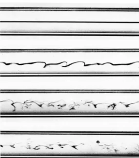
Figure 1.1: A streak of dye in a glass pipe at four Reynolds numbers, from laminar (top) to turbulent (bottom) flow. This photograph is of a recreation of Reynolds’ classic exper-iment of 1883 using the original apparatus, made by N. H. Johannesen and C. Lowe. Re-produced from the collection of Van Dyke[5]. It has long been observed that fluid flows are

either calm and viscous or energetic and chaotic. In a classic experiment [7] Reynolds found that these two states of the flow—called laminar and turbulent, respectively—could be seen in water flowing through a glass pipe by changing what became known as the Reynolds number. The Reynolds number is the non-dimensional pa-rameter that controls the transition between a laminar flow and a turbulent flow, and is written as

Re =U L

ν (1.3)

whereU and L are characteristic velocity and length scales of the flow. This parameter repre-sents the balance between inertial forces and viscous forces, which may be seen directly when equation1.2is scaled with characteristic length and velocity scales u∗= U/U , x∗= x/L , and t∗= t /(L /U ): DU∗_i Dt∗ = − 1 ρ ∂p ∂x_i∗ 1 U2+ 1 Re ∂2U_i∗ ∂x∗_j∂x∗_j (1.4) Reynolds found that for

low-Reynolds-number conditions dye injected in the flow did not mix with the flow, implying that there were steady streamlines parallel to the direction of the flow. In fact, the momentum equa-tion (also called the Navier-Stokes equaequa-tions and abbreviated as N-S) admits an analytical solution for this problem: a parabolic streamwise profile that does not vary in time or streamwise direction. However, at a certain Reynolds number this system transitions to a turbulent state, which is characterized by a time-dependent velocity profile and mixing of the injected dye, shown in figure1.1

(18)

In the years since Reynolds first quantified the differences between these two states in fluid flow many researchers have found common characteristics in a wide variety of turbulent flows. Turbulence has resisted a formal definition[8], but characteristics common to all turbulent flows include

1. Randomness: Instantaneous turbulent quantities are not predictable. The N-S equa-tion is a deterministic equaequa-tion that amplifies small perturbaequa-tions at high Reynolds numbers. This is a qualitative explanation for the two very different flow states described above—at low Reynolds numbers small perturbations are damped by viscosity, and at high Reynolds numbers these perturbations are amplified. De-terministic systems with a high sensitivity to initial conditions are not predictable. However, statistical properties of multiple realizations may be stable and predictable, i. e. the instantaneous velocity ui(xi, t ) is not predictable, but the average velocity at that point and time over many realizations—the ensemble average 〈ui(xi, t )〉 is stable and may be predicted. This quality of turbulence motivates a statistical approach. 2. Large range of interacting scales: Turbulence is characterized by a wide range of

scales, from the large scales that arise from external considerations such flow bound-aries to small scales at which dissipation occurs. Interaction between scales is non-local and non-linear, a point which will be discussed further in the following section.

3. Turbulence is dissipative and strongly diffusive: Turbulence dissipates kinetic en-ergy into heat, and is thus a thermodynamically irreversible process. Not coin-cidentally it is also very efficient at mixing. These two qualities are typically the aspects of turbulence important from a practical engineering perspective, resulting in costly turbulent friction in pipelines, but also highly effective mixing in industrial applications.

1.1.2 Turbulence theory

Lagrangian-Eulerian kinematics

The derivation of the Navier-Stokes equation for incompressible flow from first principles may be found in many textbooks[9,10], and will not be reproduced here. Explicit in this derivation is the concept of a fluid particle, i. e. an infinitesimal material element which is accelerated by forces in accordance with Newton’s second law. The fluid particle traces out a fluid-particle trajectory over time in response to external forces. If the individual fluid particles in a system of n fluid particles are arbitrarily labeled ai for i = 1...n then the material coordinate is defined as X(ai, t ). This fluid-particle path is also called a Lagrangian trajectory, and the first and second time derivatives may be taken to find the velocity and acceleration of the fluid particle

∂X(ai, t )

∂t = V(ai, t )

∂2X(ai, t )

∂t2 = A(ai, t ) (1.5)

the latter of which is simply the time history of the external forces acting on the fluid particle ai. This is the Lagrangian perspective, and arises naturally from Newtonian dynamics. Fluid particle trajectories are commonly labeled by their position x at some time t0, convieniently written as x0. For example the Lagrangian position is written as X(x0, t |t0). This labeling relates the Lagrangian and Eulerian positions as

(19)

While the fluid particle kinematics are naturally considered from a Lagrangian perspective, the forces acting on a fluid particle depend on the local spatial gradients, which are best expressed from an inertial reference frame, i. e. the Eulerian perspective. Flow variables in this perspective are defined point-wise in space and time, for example the Eulerian velocity field U(x, t ) . The Eulerian velocity is equal to the Lagrangian velocity at x = x0and t = t0

V(x0, t0|t0) = U(x, t )|x=x0, t =t0 (1.7)

a concept illustrated in the sketch shown here. This implies the general relation between Lagrangian and Eulerian expressions, written here in velocity

V(x0, t |t0) = U(X(x0, t |t0), t ) (1.8) The Lagrangian acceleration A may be expressed in terms of the Eulerian velocity field

so equation1.9may be written as A(x0, t |t0) = · ∂U(x, t ) ∂t + (U(x, t) · ∇)U(x, t) ¸ x=X(x0,t |t0) = DU(x, t ) Dt ¯ ¯ ¯ ¯ x=X(x0,t |t0) (1.12) or equivalently in completely Eulerian terms

A(x, t ) =∂U(x, t )

∂t + (U(x, t) · ∇)U(x, t) (1.13)

This development is shown here in order to stress that acceleration is a fundamentally Lagrangian quantity, and that the non-linearity of the N-S equation, the term (U · ∇)U, arises from the change in reference frame.

A statistical approach to turbulence

The random nature of turbulence motivates a statistical approach, in which the quantities of interest are not the instantaneous variables but the statistics of an ensemble of realiza-tions. A classic example of this approach is the decomposition of variables into mean and fluctuating components, e. g. the Eulerian velocity Ui(xi, t ) and pressure P(xi, t )

(20)

This decomposition is known as the Reynolds decomposition, and may be substituted into the N-S equations, here written without the explicit dependence on xi and t for convenience ∂ ∂t(〈Ui〉 + ui) + ∂ ∂xj(〈U i〉 + ui) (〈Uj〉 + uj) =−1 ρ ∂ ∂xi(〈P〉 + p) + ν ∂2 ∂xj∂xj(〈U i〉 + ui) (1.15) or ∂〈Ui〉 ∂t + ∂ui ∂t + ∂ ∂xj〈Ui〉〈Uj〉 + ∂ ∂xj ui〈Uj〉 + ∂ ∂xj〈Ui〉uj+ ∂ ∂xj uiuj = −1 ρ ∂〈P〉 ∂xi + −1 ρ ∂p ∂xi + ν ∂2〈Ui〉 ∂xj∂xj + ν ∂2ui ∂xj∂xj (1.16)

Writing the N-S equation with the Reynolds decomposition show clearly the terms that depend only on the mean flow topology, those that depend only on the fluctuating quantities, and those that depend on the interaction of the mean and fluctuating quantities. The ensemble average of equation1.16may be taken, and all terms containing a single fluctuating term go to zero by construction1, leaving

∂〈Ui〉 ∂t + ∂ ∂xj 〈Ui〉〈Uj〉 + ∂ ∂xj 〈uiuj〉 =−1 ρ ∂〈P〉 ∂xi + ν∂ 2 〈Ui〉 ∂xj∂xj (1.17)

The above equation appears to be quite similar to the unaveraged N-S equation, with the exception of the term containing the mean of the product of the fluctuating velocities, 〈uiuj〉. This quantity, called the Reynolds tensor, it is a fundamental statistical quantity in the Eulerian analysis of turbulence that has a direct effect on the mean velocity (through equation1.17), contains the turbulent kinetic energy (1₂uiui), and contains information regarding turbulent anisotropy (in the off-diagonal components).

In the frame of a fluid particle the evolution of the kinetic energy per unit mass2 E ≡1₂UiUi of the fluid particle is simply the inner product of the fluid particle velocity and acceleration

∂E(x0, t |t0)

∂t = A(x0, t |t0) · V(x0, t |t0) (1.18) In an Eulerian framework this evolution of kinetic energy is found by multiplying the N-S equation (equation1.2) by the Eulerian velocity Ui(xi, t ) as follows.

Ui DUi Dt = Ui · −1 ρ ∂p ∂xi + ν ∂2Ui ∂xj∂xj ¸ (1.19)

A Reynolds decomposition separates the energy associated with the mean flow E =1₂〈Ui〉2 and the turbulent kinetic energy k =1₂〈uiui〉. Development equations for these two quanti-ties may be formed3from equation1.19, resulting in

1_{also using the the fact that the ensemble average and differentiation operators commute.}

2_{For the flow in which density is constant it is convenient to refer to the kinetic energy as one half the}

square of the velocity, leaving the "per unit mass" implied.

(21)

1 2 ∂E ∂t + 〈Uj〉 E ∂xj | {z } Change in E + ∂ ∂xj " 〈Ui〉〈uiuj〉 + 1 ρ〈Uj〉〈P〉δi j− ν ∂E ∂xj # | {z } Transport of E = 〈uiuj〉 ∂〈Ui〉 ∂xj | {z } Production of k − ν · ∂〈Ui〉 ∂xj ∂〈Ui〉 ∂xj ¸ | {z }

Dissipation due to mean flow

(1.20) ∂k ∂t + 〈Uj〉 ∂k ∂xj | {z } Change in k + ∂ ∂xj · 〈ujuiui〉 + 1 ρ〈uip〉δi j− ν ∂k ∂xj ¸ | {z } Transport of k = −〈uiuj〉 ∂〈Ui〉 ∂xj | {z } Production of k − ν ¿ ∂ui ∂xj ∂ui ∂xj À | {z } Turbulent dissipation² (1.21) Equations1.20and1.21describe the evolution of kinetic energy in a turbulent flow, and are examined more closely in section1.2in the context of turbulent channel flow. Qualitatively, the interaction between the Reynolds stress and the mean-flow gradient transfer kinetic energy from the mean flow to the turbulence, where the kinetic energy is dissipated as heat by viscous friction. The dissipation of kinetic energy implies that a constant level of kinetic energy in a control volume requires the injection of energy into the control volume. This energy injection drives the mean flow and, by the the production term in equation1.20, injects energy into the turbulence. The structure of this energy from its injection into the turbulence to its dissipation into heat is the subject of an important theory of statistical turbulence published by Kolmogorov in 1941.

Kolmogorov’s 1941 theory of turbulence (K41)

In a series of papers4Kolmogorov proposed that in fluid turbulence with large Reynolds numbers the small scales of the turbulence becomes universal. This universality5implies a scaling based on dimensional analysis for the scales at which viscous dissipation occurs. These scales are therefore independent of the large scales in the turbulence.

η = µν3

² ¶1/4

Dissipation length scale (1.22)

τη=³ν ²

´1/2

Dissipation time scale (1.23)

u_η= (ν²)1/4 Dissipation velocity scale (1.24)

whereν is the kinematic viscosity of dimension [L]2[T]−1and ² is the mean dissipation rate of dimension [L]2

[T]−3

Further, there are range of scales small enough to be universal but too large to be affected by viscous dissipation. This inertial range is given asη ¿ l ¿ l0, where l0is the large length scale of the turbulence. Turbulence statistics in the inertial range are self-similar, i. e. they

4_{The works of Kolmogorov are introduced and put in context quite clearly by Frisch in Turbulence[}₁₁_] 5_{Which includes the assumption of local homogeneity and isotropy, more formally described as a}

(22)

depend only the scale l and of the mean rate of change of kinetic energy² . The scale l is examined precisely with the longitudinal Eulerian structure function, defined as

Sp(l ) ≡ 〈[(u(r + l, t) − u(r, t)) · l/l ]p〉 (1.25) Dimensional analysis requires

Sp(l ) = Cp²p/3lp/3 forη ¿ l ¿ l0 (1.26) Where Cp is dimensionless. For the case of p = 3 the exact result C3= −4/5 was derived directly from the Navier-Stokes equation and the assumptions of global homogeneity and isotropy. There is no similar theoretical result for the value of C2, but a large body of experimental evidence has confirmed the validity of the scaling S2∝ ²2/3l2/3. This relation may be interpreted as the amount of turbulent kinetic energy at a given length scale l .

For p 6= 3, and especially for p > 3 this scaling is complicated by the intermittency of turbulent dissipation. Refinements to K41 have been proposed, some of which are reviewed in the following section.

Kolmogorov developed this theory in the Eulerian framework, but an analogous relation was developed for the Lagrangian structure function by Obukhov and Landau[12] using the approximation6τ = r/δu(r). The Lagrangian structure function is defined as

SL_p(τ) ≡ 〈|V(x0, t0+ τ) − V(x0, t0)|p〉 (1.27) K41 predicts the scaling

SL_p(τ) ∝ (²τ)p/2 forτ_η¿ τ ¿ TL (1.28) For p = 2 the Lagrangian structure function is commonly written as

SL₂(τ) = a0²3/2ν−1/2τ2 forτ ¿ τη (1.29)

SL₂(τ) = C0²τ for τ_η¿ τ ¿ TL (1.30)

where TLis the Lagrangian time scale, and a0, C0are non-dimensional constants This scaling in the Lagrangian structure function may be seen in the Lagrangian autocorre-lation

ρL(τ) ≡ 〈V(x0, t0+ τ)V(x0, t0)〉 (1.31) using the kinematic relationship in stationary HIT:

SL₂(τ) = 2〈u2〉[1 − ρL(τ)] (1.32)

The Kolmogorov scaling in shown in equation1.30implies that ρL(τ) = 1 −a0²

3/2_ν−1/2_τ2

2〈u2_〉 forτ ¿ τη (1.33)

ρL(τ) = 1 − C0²τ

2〈u2_〉 forτη¿ τ ¿ TL (1.34)

Some results regarding the scaling of acceleration can be deduced using the kinematic relationship (valid for stationary statistics):

〈a(x0, t0+ τ)a(x0, t0)〉 = −〈u2〉 d2

dτ2ρL(τ) (1.35)

using the scaling in equations1.33-1.34the autocorrelation of acceleration is

〈a(t0+ τ)a(t0)〉 = a0²3/2ν−1/2 forτ ¿ τη (1.36)

〈a(t0+ τ)a(t0)〉 = 0 forτ À τη (1.37)

6_{Falkovich et al[}₁₃_{] offers an interesting recent discussion of the validity of this assumption and its}

(23)

Figure 1.2: Schematic view of the Kol-mogorov quadratic and linear scaling of the velocity autocorrelation.

This lack of dependence of the autocorrelation of acceleration7 on the time lagτ is reflected in the constant curvature of the velocity auto-correlation in figure1.2, and zero -correlation in the inertial range implies that acceleration is a fundamentally small-scale quantity with a time correlation approximately equal to the Kol-mogorov time scaleτ_η. The form of the auto-correlation of acceleration is not predicted from K41, although as the derivative of a stationary process the integral scale is expected to be zero in HIT[14].

The limits and extensions of K41

K41 predicts statistical similarity of velocity in-crements in the inertial range for HIT. Since the introduction of K41 many experimental results

have shown that these statistics are scale dependent. This dependence may be seen in the results of Mordant et al[1] for the Lagrangian velocity increment, shown in figure1.3. The evolution of the PDF of the normalized velocity incrementv(t0+ τ) − v(t0) fromτ ≈ TL (ap-proaching Gaussian) toτ ≈ τ_η(highly non-Gaussian) shows that these Lagrangian statistics are not self-similar in the inertial range. This lack of self-similarity is known as internal intermittency, and is known be greater in the Lagrangian framework[15]. Explanations of the behavior shown in figure1.3represent an active field of study in turbulence research.

–20 –10 0 10 20 –7 –6 –5 –4 –3 –2 –1 0

Figure 1.3: The probability density function of the normalized velocity increment for sev-eral values ofτ. The dotted line represents the distribution of acceleration. Reproduced from Mordant et al[1].

The reason why K41 fails to capture the in-termittency is that it implicitly assumes a con-stant dissipation rate in the structure function scaling shown in equation1.26; an assumption made clear by noting that 〈²p/3〉 6= 〈²〉p/3for p 6= 3 unless ² = 〈²〉. Kolmogorov and Obukhov at-tempted to address this shortcoming by con-ditioning the scaling shown in equation1.26

on the local instantaneous value of the dissipa-tion rate volume averaged on the scale l , written here as²l

〈[(u(r + l, t ) − u(r, t )) · l/l ]p|²l〉 = Cp(²ll )p/3 (1.38) and then modeling the distribution of ² as a function of scale. This approach, known as K62, is notable for two reasons. First, it directly links the instantaneous viscous dissipation—a small-scale small-scale quantity—with the small-scales in the iner-tial range. Second, it requires knowledge of the the distribution of²l, which general must be modeled and is related to the large scales of the turbulence. Kolmogorov suggested that the dissipation has a log-normal distribution, the specification of which allows the calculation of²p/3from 〈²〉. This approach has been

7_{The acceleration variance is simply equation}_1.36_at_{τ = 0, and is also referred to as the Heisenberg-Yaglom}

(24)

used to collapse Lagrangian velocity increments[16] similar to those shown in figure1.3, and used in the superstatistical approach[17,18].

Another notable approach to intermittency is the multifractal model, which models the scaling exponentζp in the Eulerian structure function

Sp(l ) ∼ lζp (1.39)

The exponentζp(p) has been shown experimentally to have the following qualities: for ζp= 1 at p = 3, confirming the exact result of Kolmogorov; approximately linear behavior at p ≤ 3, reflecting the fact that K41 provides a close approximation for lower order statistics; andζp(p) is increasingly curved for p > 3 reflecting the scale dependence of higher order statistics (e. g. the shape of the PDFs shown in figure1.3). Note that for K41ζp is linear in p: ζp= p/3 (equation1.28), and for K628predicts a curved function:ζp= p/3 + µ/18(3p − p2), whereµ ≈ 0.2 is thought to be universal.

The multifractal model attempts to predict this curvedζpin a universal manner without specifying the distribution of². The underlying idea is that turbulence has a range of fractal dimensions D that is scale dependent. The distribution of this dimension D(h), where h is the scale, is thought to be universal. As a consequence the scaling of Sp(l ) is a superposition of power laws over the range of scales:

Sp(l ) ∼ lph1l3−D(h1)+ ph2l3−D(h2)+ ...phnl3−D(hn) (1.40) D(h) is not generally known a priori, and must be modeled and/or measured directly[20]. Multifractal formalism has been extended to the Lagrangian framework and provides a unified description of turbulence in the inertial and dissipative ranges[21,22].

1.1.3 Turbulence investigations in the Lagrangian framework

As suggested by the quotation of A. N. Kolmogorov that opens this chapter, the study of turbulence has been largely driven by experimental investigation. Since the pioneer-ing experiments of Reynolds the development of experimental methods have allowed researchers to measure turbulent quantities with ever increasing spatial and temporal resolution. Historically these instruments and techniques were focused on Eulerian mea-surements; instruments and techniques enabling Lagrangian measurements in turbulence are a relatively recent9development.

Fluid particle trajectories may be measured experimentally by measuring the position of a tracer particle over time, or extracted from a direct numerical simulation (DNS) of turbulence. The experimental system used in this study, an optical particle tracking velocimetry system than uses high-speed cameras to record tracer particle positions, is fairly typical of modern experimental Lagrangian measurements. DNS solves the N-S equations directly over a large grid of positions, such that all scales of the turbulence are resolved. Fluid particle trajectories are then integrated from the calculated Eulerian velocity field that is highly resolved in x, y, z, t (See e.g. Yeung[24] for details), allowing the extraction of high resolution Lagrangian statistics. Such simulations are computationally expensive for large Reynolds numbers, but increasingly available computational resources have allowed DNS at Reynolds numbers(Re_λ= 1000) similar to many experiments[25].

8_{Following the assumption of the log-normality of}_{², see e.g. Davidson[}₁₉_{] for this derivation}

9_{With a few notable exceptions, among them a study of relative dispersion in the atmosphere by}

Richard-son in 1922[23], in which balloons were released containing messages asking the finders to note where the balloons landed and to send Richardson the location by postcard.

(25)

Turbulence statistics may be divided, somewhat arbitrarily, into the following four categories, each of which corresponds to different measurements methods, and each of which is related to different areas of turbulence research:

• One-point statistics: A measurement at a single point, e.g. by a hot-wire or pitot tube. The "frozen turbulence" hypothesis of Taylor is often used with these measurement to deduce two-point statistics.

• Many- point statistics: Simultaneous measurements at two or more loca-tions, which allow direct measurement of spatial structure. Modern optical measurement methods, such as particle image velocimetry (PIV), allow direct field measurements.

• Single-particle statistics: The trajectory of a single particle. Typically measured optically (e. g. PTV) but at low particle-seeding levels.

• Many-particle statistics: Many simultaneous trajectory, such that the measurement of particle separation distance over time, the coherence of groups of particles over time (e. g. tetrads), etc., are possible. These statistics are typically measured with techniques similar to those used to measure single-particle statistics, but they require relatively high particle-seeding levels.

Eulerian

Lagrangian

All four categories of statistics may be measured at a variety of temporal and spatial resolutions, depending on the measurement method and instrumentation used. Access to these statistics has allowed researchers to test theories and explore phenomena in turbulence. For example K41 was based on and supported by high-resolution hot wire measurements, which, using Taylor’s frozen turbulence hypothesis, furnished Eulerian structure function statistics in the inertial range. Coherent structures and their role in turbulence were elucidated using PIV measurements, which allowed spatially resolved measurements of the velocity and vorticity fields.

Similarly, the more recently available high-resolution Lagrangian measurements allow the exploration of questions regarding fluid particle velocity and acceleration. The follow-ing discussion will focus on results related to sfollow-ingle-particle statistics, which are also the focus of the present study.

Lagrangian velocity statistics in HIT K41 in the Lagrangian framework predicts

〈|V(x0, t0+ τ) − V(x0, t0)|p〉 ∝ (²τ)p/2 forτη¿ τ ¿ TL (1.41) in the limit of large Reynolds numbers, but leaves many open questions. At what range of Reynolds is this scaling observed? What are the values of the proportionality constants, especially C0?10 How is the Lagrangian timescale TLrelated to other turbulence quantities, such as more easily measured Eulerian statistics? These questions have important implica-tions for Lagrangian modeling(discussed in more depth in section1.3), as C0, TL, and Re_λ are basic ingredients of these models. A variety of experimental and DNS measurements have been reported, clearly summarized by Lien and D’Asaro[26]. A more recent DNS

10_{Where C}

(26)

from Sawford and Yeung[27] consider the second-order K41 scaling over a wide range Reynolds numbers (Re_λ= 43 − 1000). C0is found to increase with Reynolds number, even at the relatively high Reynolds that have been tested. This result is consistent with the observation that the Eulerian inertial range is greater than the Lagrangian inertial range for a given Reynolds number.

The anomalous scaling of equation1.1.3was previously evidenced in the lack of self-similarity in the PDFs of the velocity increments shown in figure1.3. This anomolous scaling is commonly written as

〈|V(x0, t0+ τ) − V(x0, t0)|p〉 ∝ (²τ)ξLp _(1.42)

Scaling exponents in the inertial range were measured directly by Mordant et al[1] and Xu et al[15], and were found to deviate more strongly from K41 (non-intermittent) values than the equivalent Eulerian exponents. While the power law scaling in equation1.42

is expected in the inertial rangeτη¿ τ ¿ TL, it does not necessarily hold whenτ ∼ τη. Biferale et al[28] and Arneodo et al[22] report measurements from several dataset of the quantity

ζp(τ) =

d log[SL_p(τ)]

d log[SL₂(τ)] (1.43)

i. e the logarithmic derivative of the structure function of order p, normalized by the logarithmic derivative of the structure function of order 2.ζp(τ) is a way of quantifying the deviation from non-intermittent behavior at each scaleτ. Both groups report strong inter-mittence atτ/τ_η≈ 2. Intermittency of Lagrangian structure functions at small time-lags is closely related to the observed intermittency of fluid particle acceleration, as Lagrangian velocity increments at small times are closely related to fluid particle acceleration by the definition a ≡ lim τ→0 v(τ) − v(0) τ (1.44) Acceleration in HIT

The acceleration of a fluid particle is proportional to the sum of the forces acting on the particle, and arises directly from the N-S equation. As such a fundamental quantity, as well as for its importance to Lagrangian stochastic modeling[29](discussed in below in section

1.3), the statistical properties of the fluid particle acceleration in turbulence have been studied extensively. Experimental[30,31] and numerical[16,32] studies have measured fluid particle accelerations, which were found to have "thick-tail", highly non-Gaussian distributions. Specifically, accelerations up to 50 times greater than the root-mean-square value have been measured[31]. The distribution of the acceleration may be inferred from the multi-fractal model, and agrees closely with experimental[31] and DNS[33] results.

The variance of acceleration has a scaling derived from K41 (equation1.37), suggesting a universal constant a0exists at high Reynolds numbers. Sawford et al[34] assembled a several datasets to examine the dependence of a0on Reynolds number, and did not find evidence that a0is independent of Re_λfor Re_λ< 1000.

The autocorrelations of acceleration components were found to have short decorre-lation times with respect to the autocorredecorre-lation of the magnitude of acceleration[35,16]. Evidence for a connection between intense acceleration events and vortex filaments[36] suggests the difference between the correlation times of an acceleration component and the acceleration magnitude may be explained vortex trapping: in which a fluid particle has a relatively long-lived helical motion that follows a small vortical structure. As the particle

(27)

moves around the axis of rotation of the vortex, the acceleration direction decorrelates rapidly, but the acceleration magnitude stays relatively correlated. Further evidence of that vortex filaments are related to the intermittency of acceleration was reported by Toschi et al[37], who found that the component of the acceleration perpendicular to the velocity has different statistical properties than the component of acceleration parallel to the velocity. Specifically, intense acceleration events in the perpendicular component are correlated over a greater time than intense events in the parallel component.

In the vision of Kolmogorov, high Reynolds number turbulence is characterized by scale-separation; large scales are decoupled from small-scales. This suggests that veloc-ity (associated with the large scales) and acceleration (associated with the small scales) are independent of each other. This assumption is implicit in second-order Lagrangian stochastic models[38,39], which model acceleration and velocity as independent processes. In fact, several studies have shown strong dependence of the acceleration variance on velocity. Crawford et al[40] report experimental results showing that intense accelerations are correlated with high velocities in high Reynolds number turbulence. The dependence is shown to increase with Reynolds number, which is counterintuitive given the increased scale-separation at higher Reynolds numbers.

1.2 Turbulent Channel Flow

Figure 1.4: Schematic of a turbulent channel with coordinate system. A high aspect ratio (h ¿ W) and sufficient de-velopment length (h ¿ L) ensure statis-tical homogeneity in the streamwise(x) and spanwise (z) direction.

The previous section focused on the theory and pre-vious work related to HIT, with a focus on investiga-tions from a Lagrangian perspective. Similar inves-tigations in inhomogeneous turbulence are much less common due to the theoretical and experimen-tal/numerical complications associated with the in-homogeneity. However, inhomogeneous turbulence is ubiquitous in nature and engineering, motivating a deeper understanding of such turbulent systems. Technological advances in high-speed cameras and computing power increasingly allow experimental and numerical Lagrangian investigations of such tur-bulent flows. In order to limit the complexity intro-duced by the inhomogeneity there is a preference for "simple" inhomogeneous turbulence flows, such as turbulent channel flow. This section introduces turbulent channel flow, and describes selected char-acteristics of this flow relevant to the work presented in this thesis.

Turbulent channel flow is an internal, pressure-driven flow in a rectangular channel at sufficiently high Reynolds number. If the channel is sufficiently long and sufficiently high-aspect-ratio, the flow is homogeneous in the streamwise (x) and spanwise (z) directions; the only direction of inhomogeneity is the wall-normal (y) direction11. As such it is a convenient academic framework to study inhomogeneous turbulence.

By symmetry all statistics, e. g. the mean streamwise velocity, are symmetric about the

11_{This assumption is often implicit in the literature of turbulent channel flows, i. e. "turbulent channel}

(28)

mid-plane of the channel y = h

〈Ux(x, y∗, z)〉 = 〈Ux(x, 2h − y∗, z)〉 0 < y∗< 2h (1.45) Statistical homogeneity in the streamwise and spanwise direction, and the conservation of mass and momentum give the following results for the mean Eulerian velocity and pressure fields: 〈Uy(x, y, z)〉 = 0 (1.46) 〈Uz(x, y, z)〉 = 0 (1.47) ¿ d P(x, y, z) d x À = constant (1.48)

This constant streamwise mean pressure gradient drives the flow, and in stationary flow is balanced by the wall shear stressτw. The wall shear stress provides a convenient quantity by which to scale flow variables. Following the notation of Pope[10] this scaling is given as

u_τ=s τw ρ Velocity wall-scale (1.49) δν=ν r ρ τw Length wall-scale (1.50) t_τ= νρ τw Time wall-scale (1.51)

These wall-scales are used to scale flow variables, which are then denoted with a "+" superscript, e. g.

y+= y

δν (1.52)

The Reynolds number typically chosen to characterize turbulent channel flows is formed with this velocity wall-scale as

Re_τ≡uτh ν Eqns. 1.49,1.50 = h δν (1.53)

This definition of the Reynolds number is convenient in that is gives a direct measure of length scale separation between the viscous wall length scale (δν) and the largest length scale (h).

High Reynolds number channel flow varies qualitatively with respect to the distance from the wall (y+). Attempts to describe and understand this variation from a purely statistical point of view has occupied researchers since Prandtl, and have led to advances such as the law of the wall and an understanding of the production-transport-dissipation of turbulent kinetic energy in the system. Another approach12focuses on the organization of vortical flow structures in the channel , and their role in the turbulence. A small selection of results from each approach are discussed here.

1.2.1 Eulerian statistics in a turbulent channel

Law of the wall

Dimensional analysis using the assumptions made above lead to the expression for the mean shear d 〈U+ x〉 d y = 1 y+f µ y δν, y h ¶ (1.54)

12_Tsinober[₈_{] points out that it is impossible to draw a clear line between a "statistical" and a "structural"}

(29)

At high Reynolds number one may assume that there is a distance from the wallδν¿ y ¿ h such that the mean shear is independent of bothδ_νand h, in which case the function f must be a constant, i. e. d 〈U+x〉 d y = 1 κy+ forδν¿ y ¿ h ⇒ 〈U+x〉 = 1 κl n(y+) + B for δν¿ y ¿ h (1.55)

whereκ is the von Kármán constant (≈ 0.41) and B ≈ 5.2 for smooth walls. The layer in which this self-similar relation holds is called the log layer. Very close to the wall the dynamics are dominated by viscous stress, and between these two layers there is a transitional layer called the buffer layer. These three layers are defined13as

Viscous layer: 0 < y+< 5 (1.56)

Buffer layer: 5 < y+< 30 (1.57)

Log layer: y+> 30, y/h < 0.3 (1.58) and are shown graphically with the mean velocity and velocity variance in figure 1.5. Note that peak of the streamwise variance occurs in the buffer layer, as does the peaks of turbulence production, dissipation, and turbulent kinetic energy (not shown in figure1.5), highlighting the dynamical importance of this layer, despite how little of the channel it fills (less than 2% of the half-width of the channel at Re_τ= 1440). The definition of the log-layer layer illustrates how the width of this layer depends on the Reynolds number

Lower limit of log layer: y+= 30 = 30 h

Re_τ Upper limit of log layer: 0.3h (1.59) i. e. for a given channel width h the upper limit of the log layer is fixed, and increasing Re_τ acts to shrink the viscous length scale, thus pushing the lower limit of the log layer towards the wall.

Dimensional analysis similar to the derivation of the log law (equation1.55) gives U0− 〈Ux〉 u_τ = − 1 κl n ³y h ´ + B1 for y ¿ h (1.60)

where U0is the mean streamwise velocity at the centerline (U0= 〈Ux(y)〉|y=h), and B1is a constant (≈ 0.2). Equations1.55and1.60can be combined yielding

U0 u_τ = 1 κl n µ Re0 u_τ U0 ¶ + B + B1 (1.61)

which relates the ratio of velocity scales to the large-scale Reynolds number Re0≡ U0h/ν. This relation allows the estimation of the velocity scale u_τ directly from the centerline velocity, which is more practical experimentally, as a direct measurement ofτw is often not possible.

Reynolds stresses: production, transport, and dissipation

The equation governing the kinetic energy in a turbulent flow, U · h DU Dt = − 1 ρd Pd x+ ν∇ 2_Ui_, was previously developed using the Reynolds decomposition (equations1.20and1.21).

13_{This definition is taken from Pope[}₁₀_{], but definitions vary in the literature, e.g. Hoyas[}₄₁_{] take the log}

(30)

Buﬀer Layer Log Layer Viscous Layer Buﬀer Layer Log Layer Viscous Layer

Figure 1.5: Profiles of mean streamwise velocity (left) and component-wise velocity variance (right), shown with the viscous layer, the buffer layer, and the log layer. Red symbols are experimental data, green symbols and black line are DNS. Velocity variance profiles are offset by 5u2_τfor clarity. Figure modified from Stelzenmuller et al[42].

Using the symmetries of turbulent channel flow, these equations are simplified to

∂ ∂y " 〈Ux〉〈uxuy〉 − ν ∂E ∂y # +1 ρ ∂〈P〉 ∂x 〈Ux〉 | {z } Transport of E = 〈uxuy〉 ∂〈Ux〉 ∂y | {z } Production of k − ν · ∂〈Ux〉 ∂y ∂〈Ux〉 ∂y ¸ | {z }

Dissipation due to mean flow

(1.62) ∂〈uyuxux〉 ∂y | {z } Turbulent transport + 1 ρ ∂〈uyp〉 ∂y | {z } Pressure transport − ν∂ 2_k ∂y2 | {z } Viscous transport = −〈uxuy〉 ∂〈Ux〉 ∂y | {z } Production of k − ν ¿ ∂ui ∂xj ∂ui ∂xj À | {z } Turbulent dissipation² (1.63) where E =1₂〈Ux〉2and k =1₂(u2x+ u2y+ u2z). Some of the terms in these energy equations are easily measured experimentally, and will be presented in Chapter3. Other terms, such as the fluctuating spatial velocity gradients and the fluctuating pressure, are generally not accessible in experiments. Results from DNS[43,44], where all of the terms can be directly measured, have been published for a range of Reynolds numbers. The profiles of these terms across the channel show the following behavior in each layer.

• Viscous layer: In the viscous layer there is very little fluctuating velocity and thus very little production. Dissipation is highest at the wall, balanced by viscous transport term which brings energy towards the wall.

• Buffer layer: In the buffer layer all of the terms in equation1.63 are important. The production term is highest in this layer, and is greater than the dissipation, which means the transport terms are working to bring energy toward the wall (by the viscous transport term) and away from the wall (by the pressure and turbulent transport term). The viscous and buffer layers have been shown to be dependent on the Reynolds number.

• Log layer: In the log layer the production and dissipation of energy are in balance, and the transport terms become negligible. The wall-scaled terms show little depen-dence on Reynolds number.

(31)

• Beyond the log layer: Between the log layer and the channel centerline the produc-tion declines to zero, and the dissipaproduc-tion is balanced by the transport terms.

Anisotropy

Turbulent channel flow is characterized by a high degree of anisotropy. The mean velocity is highly sheared, and the variance of fluctuating velocity components—〈ux2〉, 〈u2y〉, 〈uz2〉— differ significantly. These large-scale anisotropies are greatest near the wall, and relax to isotropy at the channel centerline. It remains an open question as to the extent to which the small scales of the flow are isotropic in the high Reynolds number limit, as predicted by Kolmogorov. In a turbulent channel DNS of Re_τ= 1000, Pumir et al[45] found small-scale anisotropy up to the channel center, by some measures greater than that found in equivalent homogeneous shear turbulent flow. In another channel flow DNS at a similar Reynolds number Zamansky et al[3] found that the orientations of acceleration approach isotropy at y+≈ 40, i. e. the beginning of the log layer.

1.2.2 Vortical structures in a turbulent channel

Figure 1.6: Sketch of a horseshoe vortex, showing two parallel streamwise legs close to the wall and spanwise elevated head. Reproduced from Adrian[2]. Flow visualization techniques applied to

wall-bounded turbulence have revealed organized mo-tions in the turbulence. These organized momo-tions have been studied extensively[2, 46, 47, 48], al-though there is a general lack of agreement in the literature about how to define these organized mo-tions. For the purpose of this discussion an intuitive definition of a vortex will suffice.

Herpin et al[49] analyzed data from a channel flow DNS (Re_τ ≈ 950) with respect to the num-ber and radii of vortices across the channel width. Streamwise vortices were found to be significantly more common than spanwise vortices in the buffer and log layers. This difference is minor beyond the log layer, but a small difference persists almost to the channel center. The overall number of vortices peaks at y+≈ 100 for both streamwise and spanwise vortices, and declines towards the center. Stream-wise vortex radii were found to be smaller than those of the spanwise vortices in the near-wall region, and approximately equal elsewhere.

The qualitative picture given by these results is that turbulence near the center of the channel—3-D, quasi-isotropic, quasi-homogeneous turbulence—becomes more and more organized as one approaches the wall. This organization manifests as vortices increasingly aligned in the streamwise direction, i. e. a system between fully 3-D HIT and 2-D turbulence14. From a Lagrangian point of view, one in which high accelerations events and the long time correlations of acceleration magnitude are associated with fluid particles "trapped" in vortices, the organization of vortices is expected to have a significant effect on Lagrangian statistics.

14_{Clearly near wall turbulence is quite different from classical 2-D turbulence, but there are intriguing}