HAL Id: hal-01470232
https://hal-amu.archives-ouvertes.fr/hal-01470232
Submitted on 17 Feb 2017HAL is a multi-disciplinary open access archive for the deposit and dissemination of sci-entific research documents, whether they are pub-lished or not. The documents may come from teaching and research institutions in France or abroad, or from public or private research centers.
L’archive ouverte pluridisciplinaire HAL, est destinée au dépôt et à la diffusion de documents scientifiques de niveau recherche, publiés ou non, émanant des établissements d’enseignement et de recherche français ou étrangers, des laboratoires publics ou privés.
LOCAL REACTIONS TO THE FINANCIAL CRISIS:
WHAT INFLUENCE OF NATIONAL CONTEXT VS
INDIVIDUAL STRATEGIES?
Céline Du Boys, Emanuele Padovani
To cite this version:
Céline Du Boys, Emanuele Padovani. LOCAL REACTIONS TO THE FINANCIAL CRISIS: WHAT INFLUENCE OF NATIONAL CONTEXT VS INDIVIDUAL STRATEGIES? : A COMPARATIVE STUDY ON THE EFFECT OF THE 2008 CRISIS ON FRENCH AND ITALIAN MUNICIPALITIES. EGPA (European Group for Public Administration) Annual Meeting, EGPA (European Group for Public Administration) Aug 2016, UItrecht, Netherlands. �hal-01470232�
LOCAL REACTIONS TO THE FINANCIAL CRISIS:
WHAT INFLUENCE OF NATIONAL CONTEXT VS INDIVIDUAL
STRATEGIES?
A COMPARATIVE STUDY ON THE EFFECT OF THE 2008 CRISIS
ON FRENCH AND ITALIAN MUNICIPALITIES.
Céline DU BOYS Associate Professor Aix Marseille Univ, CERGAM – IMPGT, Aix en Provence, France Institut de Management Public et Gouvernance Territoriale celine.duboys@univ-amu.fr Emanuele PADOVANI Associate Professor Department of Management, University of Bologna, Italy emanuele.padovani@unibo.it 2016 EGPA Annual Conference 24-26 August – Utrecht, Netherlands This is a working paper: Please do not cite without permission from authors1 Introduction
The 2008 crisis has damaged or weakened most European Local Governments (LGs)’ financial situation. The shock has been more or less intense depending on the national context and policies, and on individual situations and strategies. After the crisis, different and successive types of recovery plans, austerity measures, and institutional reforms have been implemented by States (Kickert 2012; Schick 2011), with several diverse effects on LGs’ situation (for example Cepiku et al. 2015). The previous situation of LGs in terms of financial autonomy, State protection or local responsibilities and actions also influenced their post crisis situation, not to mention the provision of bankruptcy in certain nations (Scorsone and Padovani 2014).
At the individual level, depending on their size and capacities, LGs followed different strategies to cope with the crisis and the decrease in public resources. Taking a short or longer term perspective, LGs have had various options: from brutal cost cuts (Raudla 2013) to more elaborated restructuring of their actions and missions, even by outsourcing to the private sector, to other governments via public-public partnerships or by adopting several other organizational schemes (Savas 1987); from basic fiscal leverage to new strategies for enhancing revenues (Carroll and Johnson 2010).
Consequently, LGs show various patterns of resilience and different long term capacities to cope with other shocks or crisis. While the effects of central measures and reforms on LGs have already been studied at a macroeconomic perspective – i.e. considering LGs as a whole or as a sub-sector of public administration – a few attention has been given to the effects on LGs considered individually. As part of a wider research, this paper is a first attempt to understand the influence of national contextual factors and individual characteristics in the LGs reaction to the 2008 crisis. The cross country comparative analysis provides the opportunity to isolate the effects of the national context. The paper aims at describing the evolution of the main municipal financial balance factors and the arbitrage made in terms of current revenues, current expenditures and capital expenditures throughout the 2008 crisis, and between France and Italy. It also analyzes the effect of the size of municipalities on these variables. This research is intended to answer the call for comparative studies on how different nations have reacted to global crisis (Pollitt 2010; Raudla 2013) covering the specific level of LGs. To do so, we propose some descriptive statistics and some simple linear relation tests on a panel of 225 municipalities overs 50.000 inhabitants in France and in Italy, throughout the 2004 to 2014 years. Our results shed light on the effect of institutional context and on the timing of the crisis between France and Italy. For example, one may wonder whether the late decrease in state grants to municipalities, coupled with the tax guarantee on tax payment and the absence of any bankruptcy regulation have postponed the effect of crisis in France and how this differentiates from Italy. Interesting comparative perspectives may also be useful to understand whether certain policies have been effective and, if so, to what extent. Finally, our results illustrate the effect of size (and thus the level of expertise of managers and elected representatives) on municipal reactions to crisis. This paper is at its first stage. It reports the first step of a larger research that aims at providing a quantitative overview to answer the research questions above. Thus, we are here only providing some descriptive statistics and simple linear analysis. This paper is structured as follow. Section 2 discusses the conceptual framework that we use in this study. Section 3 describes the main national institutional relevant profiles of the two contexts, France and Italy. The
methodological approach used is presented in Section 4, while Section 5 contains the analysis of our data and some discussions. We then draft some first conclusions with the analysis at hand.
2 Conceptual framework
This research locates at the intersection of two streams of research, namely the effects of the global financial crisis on LGs and the measurement of LGs’ financial health. Our conceptual framework is used to logically organize relevant literature and builds upon a qualitative research approach on management of austerity in LGs by Cepiku et al. (2015). This is then applied to our quantitative analysis of municipalities in France and Italy. As this is a first stage of research, the conceptual framework is only partially applied.
We are interested to investigate how financial health (our final dependent variable) – sometimes called financial condition or fiscal health – has been influenced by different arbitrages made in terms of expenditures and revenues (our intermediate dependent variable) on the basis of the forces that influence LGs’ reaction to crisis. Literature singles out three different types of forces (our three independent variables): economic and social factors, national institutional contextual factors, and internal factors. The conceptual framework is represented Table 1. Table 1 – Conceptual framework
2.1 Forces that influence LGs’ reaction to crisis
The reaction to crisis is dependent mainly from such economic and social factors as economic growth, unemployment and income levels; its level of severity and length affects with different magnitude (the higher the worst) both revenues through tax base reduction and expenditures via an increase of demand for services (Dunsire and Hood 1989; Pollitt 2012; Raudla et al. 2013).
National institutional contextual factors that affect LGs’ reaction to crisis can be seen at three different levels: the administrative culture or traditions (Loughlin 1994), the basic structure of the sate in terms of vertical dispersion of authority (Pollitt and Bouckaert 2011), and the state-level austerity policies in reaction to crisis (Miller and
Economic and social factors National institutional contextual factors Internal factors Forces that influence LGs’ reaction to crisis Approach to crisis by arbitrage of revenues and expenditures Financial health
Hokenstad 2014). France and Italy can be considered similar in terms of culture or administrative traditions (Ongaro 2010), therefore we can limit our analysis to the other two variables. The vertical dispersion of authority relates to the different state models. While usually the distinction is between unitary and federal states, some unitary states are so highly decentralized that the degree of de facto decentralization is even higher than in federal state. It is thus important to distinguish between different levels of centralization/decentralization. The concept of decentralization is multifaceted and complex in nature. Schneider (2003) defines three types of decentralization: fiscal, administrative and political. The measurement of centralization/decentralization is controversial, but amongst the most popular measures that have been used there are share of revenues or expenditures at local level compared to the public sector, percentage of local revenues controlled by LGs, and percentage share of public employment.
One element that may be considered as symptom of high level of autonomy and thus high decentralization is the presence of bankruptcy rules opposed to state takeovers. Bankruptcy refers to that situation where a LG’s state of insolvency is declared or imposed by a court order, and creditors are paid by clearance of assets and credits. Many countries do not have a provision for LG’s bankruptcy filing but rather a higher level, usually the central government, takes charge of the situation. The United States represents one of the major examples, even though recent research demonstrates that it is a complex and multidimensional process where the causes behind jurisdictions that fall into bankruptcy are varied and no simple linear relationship exists (Scorsone and Padovani 2014).
Another aspect that is important to assess the level of freedom of a LG, and thus its subjection to national policies, is its ability to decide their budget policies amongst which debt burden is pivotal. Most countries (but not all) provide restrictions to LGs borrowing. Policies affecting the debt load (by limiting borrowing so as to reduce debt load or by taking direct control of the financial load), policies affecting current primary savings (by restricting borrowing to finance capital expenditure or by increasing municipal revenues), or policies affecting the co-funding efforts (by reducing co-funding of investments or reducing capital expenditures) are possible strategies put in place by State governments (Cabases et al. 2007).
The introduction or strengthening of debt borrowing limits may be provided in answer to a crisis. State-level austerity policies that affect LGs come in different forms. Standardization of procedures, setting limits and ceilings to spending, borrowing and activities, general priority-setting by the government are the main example of state-level austerity policies that inevitably brings to a higher centralization in the relationship between central and local governments (Stanley 1980; Peters 2011; Pollitt 2010). While the rational and the deliberate goals of these procedures are set to face fiscal crisis, contradictions exist (Cepiku and Bonomi Savignon 2012) and these policies may not have the desired impact on revenues, costs and debt (and thus the financial health of LGs).
Finally internal factors constitute an important set of forces the influence LGs’ reaction to crisis. Financial autonomy, budget flexibility and degree of fiscal distress have been detected as determinant (Lee et al. 2009; Pollitt 2012). Barbera et al. (2016) argue that previous financial conditions have an impact on responses to crisis by city governments’ decision makers. For example an ex-ante situation of structural surpluses tend to postpone cutbacks. Leadership and managerial capacities are other determinant internal factors. Their presence is considered pivotal as they minimize the negative effects of cutbacks (Behn 1980; Levine 1978) and may develop long-term strategies in answer to crisis, including infrastructure development and employment retraining (Pollitt 2012).
2.2 Approach to crisis by arbitrage of revenues and expenditures
Municipalities seem to react to crisis and austerity by implementing several patterns of responses, from reorientation, when municipalities consider a crisis as an opportunity for imprinting a reorientation toward a stronger financial health, to buffering, when municipalities have accumulated surpluses from past periods of abundance; from continuous adjustment, in case LGs show a strong planning and control culture together with a conservative approach to spending, to avoiding problems and catching opportunities, when governments are familiar with a day-to-day and emerging financial strategy (Barbera et al. 2016). Our intermediate dependent variables capture these responses of LGs by their impact on revenues, costs and debt.
As far as revenues are concerned, LGs may react in several ways. Notably a portion of their inflows of financial resources is decided by the central state that, during financial crisis, is reduced. This may be not only with reference to grants, but also the national government can limit the possibility by LGs to impose new local taxes or can limit the raise of tax rates or impose modifications to tax bases. But, of course, LGs retain rooms for manoeuvre for their revenues for example by deciding the prices of their fee-paying services. Raises in local revenues in reaction to state grants decreases may occur especially in the early phases of crisis, when the “tooth fairy syndrome”, i.e. the idea that cutbacks are not needed, may influence LGs decision makers (Levine 1979), or in case the cutbacks provided are less than the reduction of state grants. There is a wide body of studies that has focused its attention on the pattern of expenditure cutback, but the most important appear to be capital spending reduction and personnel expenditure reduction via hiring freeze. Capital spending has been considered being the prevalent expenditure being cut during crises (Levine et al. 1991, Dunsire and Hood 1989). Capital spending cancellation or freeze seem to be the most common, but not necessarily the most promising in the long term, strategy for facing financial resource scarcity (Scorsone and Plerhoples 2010). Another “freezing” strategy is adopted for personnel hiring, as it contributes to decrease expenditures without unpopular layoffs (Levine 1978; Rubin 1985). As final possibility there is real reduction of operating expenditures via cuts of programs or efficiency increase.
2.3 Measuring and comparing financial health internationally
Comparing the financial performance and condition of LGs has been an aspect widely discussed when the comparison is limited within nations, while less attention has been received when extended across national boundaries (Padovani and Scorsone 2011). This topic calls for several types of issues that have been already examined in literature. First of all its should be noted that reporting of public finances – LGs included – is at the cornerstone of two competing approaches to accounting: “government financial statistics” otherwise called “national statistics”, i.e. that accounting system whose aim is to represent economy at a whole and articulated in its subsectors, and “government financial reporting”, whose foundational basis is entity accounts. The former of these two approaches is macro and generally used at the national level to compare public finances internationally, whereas the latter is micro and used at the local level. This creates differences in the accounting numbers provided and reflects the interests, stakes and, above all, “languages” of two competing communities, respectively that of national statistic offices and international governmental institutions (e.g. United Nations, International Monetary Fund, Eurostat) on one hand, and that of private actors, professional standard setters, professional accountancy bodies, and audit firms on the other. In this research, we focus on the “government
financial reporting” approach as our unit of analysis is each municipality (micro) instead of the system of municipalities (macro).
For the “government financial reporting” the International Public Sector Accounting Standard Board (IPSASB) provides a set of standards (IPSAS) that have been followed by several countries around the world, but only a limited number of EU countries have applied them and with different nuances (Ernst & Young 2012, PricewaterhouseCoopers 2014). Accrual accounting is at the core of these standards and its adoption in government financial reporting has been considered one of the pillars of the New Public Management paradigm and an unquestionable goal for public sector organizations even though facing difficulties (Lapsley et al. 2009; Pina et al. 2009). This has progressively pushed governments to move from traditional cash accounting systems towards accrual accounting. This has created several domestic complex processes that continue for several years with the aim to define standards according to specific objectives, by specific stakeholders, and using several pathways of implementation of new accounting systems (European Parliament 2015). For example, with reference to the two countries included in this study, French LGs have a level of proximity of their accounting information to IPSAS of 84 percent while Italian LGs got a lesser level, 30 percent (Ernst & Young 2012).
Accounting plays a pivotal role in providing comparable information, but to understand and compare financial condition and performance of LGs it is appropriate to single out a limited set of key performance indicators (KPIs). The literature concerning financial condition KPIs used to measure financial health in LGs is quite limited in number and, with a few exceptions, is restricted to the U.S. and Australian contexts and to municipal government types. This literature tends to highlight the negative side of financial health by studying the concepts of “fiscal distress”, “financial risk”, “fiscal crisis”, or “fiscal strain”. Broadly speaking, financial health can be seen as the condition in which a local government is regularly able to meet its payroll, pay its current liabilities, meet its debt service (Downing 1991, 323), and undertake service obligations as demanded by constituents (Falconer 1991, 812; Krueathep 2010, 224); the American Governmental Accounting Standards Board uses the word “economic condition” to summarize a composite situation of financial health and ability and willingness to meet financial obligations and commitments to provide services (Mead 2006). Groves and Valente (2003) have singled out four generally agreed upon sub-concepts of financial health, i.e. cash solvency, budget solvency, long run solvency, and service level solvency. While some researchers have argued that the comparability of financial reports and accounts may be achieved only at a rhetorical level (Heald and Hodges 2015), a recent research project has defined a common framework that make the international comparison of city governments’ financial health possible. Originating from currently used accounting information and a process of selection and legitimization of information upon which comparing LGs, the results point out that relevant information to compare city governments’ financial health is to a great extent already available but needs to be interpreted and “re-shaped” for purposes of making comparisons (Padovani and Heichlinger 2016).
3 Municipalities in Italy and France: national institutional
contextual factors
This section follows previous research by the authors (Du Boys et al. 2014) that have identified, through a qualitative study, some important differences in the French and Italian institutional contexts that describe the level of central authority on municipal finances and the state-level austerity policies enacted to face the crisis.
3.1 France: central authority on municipal finances
The French Republic is a unitary State which organization is decentralized, as regard to article one of the Constitution. The three levels of LGs (region, department and municipality) have a very similar legal system, and are placed on an equal footing regarding the State. They are freely administrated by elected councils, and do not exert control on each other. In 2015, there were 36.658 municipalities (communes), but only 958 over 10 000 inhabitants, describing a highly fragmented pattern. Municipalities have extensive autonomous powers to implement national policy and are responsible to manage such services as waste collection and disposal, water and sewerage systems, roads, social services, building permits and planning. Municipal taxes are collected directly and indirectly from citizens and companies. Municipalities’ councils vote the rate of main direct taxes, and the State ensures the tax collection and bears the risk of non-payment. The State pre-pays and guarantees the amount of taxes voted locally. This service to LGs is often seen as the counterpart of the cash deposit obligation to the Treasury account (Mouzet 2011). Full accrual accounting is applied both to general accounting and budget. The local public representative (such as the mayor for municipalities) establishes an administrative account which traces the budgetary flows of the past year. The accounting officer (who is a member of the State accounting department) establishes the balance sheet and the cash flow statement. LGs must also produce a statement of their off-balance sheet commitments, and the list of funded organizations where they took on liabilities, such as associations. However, no consolidation of accounts is required.
Budget must be balanced. Budget is split in two sections: current or operating activities and capital ones. Operating section can generate a surplus, which will permit to finance the investment activities. The implementation of the budget may still give rise to a deficit. In that case, measures to restore equilibrium must be implemented in the following budget. The Prefect and the Court of Auditors, representing the central state, monitor or impose measures to return to the balance. Borrowing is only allowed for investments, not for operating activities. Debt repayment is mandatory and must be done from own-resources. Many LGs suffer from a risky debt structure due to an important proportion of toxic loans1. There is no systemic risk (Observatoire des finances locales, 2014), but many LGs are affected and some suffer from a high increase in their financial expenses. The loan agreement with a bank is a matter of private law, but includes a commitment to increase taxes if necessary to fulfil the annual repayments (Mouzet, 2011). Since 2011, LGs are facing a reduction in loan offers: less volume and duration and an increase in bank margin. Today, LGs’ loans seldom exceed 20 years (Girardon, 2011). But the European Investment Bank and the Caisse des Dépôts et Consignations initiatives have offered to cover LGs long-term investments with loans from 20 to 40 years (Observatoire des finances locales, 2014), perhaps anticipating some possible future distress. In fact, evidence shows that local debt is low, but is increasing since 2003 and reached 115,4 billion in 2013, of which 62,9 (or 3,2% of national public debt) is generated by municipalities. From 2008 to 2011, LGs were limited by the bad market liquidity and attempted to limit their debt growth. The 2012 debt market’s dynamism pushed LGs to increase debt again.
Local authorities mainly use bank financing (over 97% in 2011), but they have the right to issue bonds
Bond market will be more open to LGs, thanks to the creation, in 2013, of a dedicated financing agency, Agence France Locale. Its mission is to borrow directly on the financial markets and to grant loans to its shareholders (Observatoire des finances locales, 2014). Bankruptcy procedure does not apply to LGs and their assets are exempted from seizure. Specific procedures are designed to protect creditors. Thanks to these mechanisms, the risk of insolvency does not seem to exist in LGs. Even in the worst examples of French LGs difficulties, there has been no debt write-off. The debt has just been extended to enable the payment. 3.1.1 France: State-level austerity policies After the 2008 crisis, successive national economic recovery plans (26 billion euros in 2009 and 35 billion euros in 2010) that limited the economic recession. In 2010, specific measures are implemented to support local investment.
At the same time in 2010 (after years of less intense local revenues reforms) the removal of an important business tax called “Taxe professionnelle”2 resulted in a great loss of flexibility in revenues and has been a
challenge for LGs. But then, austerity measures to force LGs to rationalize their expenses, passes through decrease in the “DGF”, the main general operating grant: - From 2011 to 2013: freeze of the DGF - In 2014, a 1,5 billion decrease in DGF. - From 2015 to 2017, a 11 billion decrease in DGF. It has been felt as strong and unexpected shock for most LGs. In 2017, the DGF will have decreased by 28% from 2011.
3.2 Italy: central authority on municipal finances
The Italian Constitution recognizes federalism and localism. Italy has a fragmented LGs pattern, with three main governmental levels, the State level, the regional level, and the municipal level. The previous fourth level (between regions and municipalities) has been transformed in a second tier LG, a sort of consortium amongst municipalities. In common they all have a territorial basis of action. As to municipalities, the constitution provides a certain level of autonomy in terms of ability to raise taxes and service fees, for which they are responsible in terms of collection, decide on the organization and performance of their functions and offices, and allocate resources to different functions and services provide. There are ca. 8.100 municipalities (comuni) that are responsible for such local services as local transportation, waste collection and disposal, social services, road and school infrastructure and maintenance.In 2009 a law has been issued and become the cornerstone of the fiscal federalism reform of Italian public administration, by defining the principles and steering criteria to execute fiscal federalism by delegating the government to reframe the financial relationships between the central State, regions and LGs, with the general
2 Tax paid by businesses, based on the value of their fixed assets. The rate was set by LGs. It represented 44% of LGs’ tax
revenues. It has been replaced by several taxes which are smaller in amount. Moreover, some of them are very volatile and their rate is not set by the LG.
aim to foster LGs’ autonomy and accountability. This is an all-encompassing, still on-going reform. In general, the Italian Constitution provides for financial autonomy of LGs, which is regulated by specific laws, decrees and regulations, according to self-sufficiency, financial autonomy, equalization and state intervention principles. Nevertheless, today the system appears contradictory since even though LGs have been provided by a pronounced financial autonomy, the central government is conferred a high power over local finances, particularly during economic crisis. The most important municipal taxes are property tax and a percentage of the national income tax, plus services fees (especially trash collection and disposal fees).
Unfortunately during the period covered the central government provided a schizophrenic changeable situation where the property tax was one of the most important sources of local revenues until 2007, then it has been replaced by government funding, then back to a higher property tax in 2012 and finally the abolishment of property tax for main residences in 2013, with replacement by a state fund; furthermore, the possibility to use the municipal personal income tax has been frozen between 2009 and 2012, determining a strong re-centralization of fiscal finances between 2008 and 2011. More than in reaction to crisis, this relates to the political instability of the country and the different visions of public (local) finances by political parties.
Starting from 2009, the Italian public sector accounting has been challenged by an all-encompassing reform called “harmonization of accounting systems and reports”. The goal of this harmonization is to favor a horizontal reading of public financial reports, overcoming the current fragmentation caused by the adoption of different criteria between different levels of Italian public administration, and fostering the development of an integrated accounting system suitable for the consolidation of public accounts satisfying the economic and financial demands of the EU. During the period covered by the analysis and still currently, accounting rules frameworks adopted in the different sectors of the Italian public administration varies considerably. Municipalities are provided by a cash/modified cash plus modified accrual bases of accounting sometimes called commitment-based accounting accompanied by an accrual basis-like set of documents. This policy cannot be considered as in answer to the global crisis of 2008 as it was pushed by political arguments made well before the crisis arose. Similar to France, the municipal budget is divided into operating and capital revenues and expenditures with the former one that can a surplus to finance capital expenditures, and any overall imbalance must be covered in the following budget cycle. The Court of Auditors, representing the central state, monitors or suggests measures to balance. Municipal borrowing was 2,1% of the Italian public debt and has decreased during the last years (for example, in 2010 it was 2,7% - source: Bank of Italy). It is subjected to specific restrictions by Constitution, national and regional laws with the aim to guarantee financial sustainability. Municipal debt is mainly represented by loans (84,4%), while the remaining part is composed by municipal bonds (13,8%) and other marginal forms (1,8%) (Corte dei conti 2014). LGs (especially those located in the South) may have benefited of debts repaid by the State to finance specific infrastructures. Revenue factoring or other forms of credit lines that allow to overcome temporary lack of cash to pay for expenses already covered by budgeted resources, are temporarily possible and not accounted as public debt. The law imposes quantitative limits to borrowing related to annual revenues. LGs can take out new debt in case the new annual amount of expenses for interests (of any form of past and new debt and guarantee) does not exceed a specific amount of current revenues of the second to last previous fiscal year. The length of any debt operation (even for renegotiations) is between a minimum of 5 to a maximum of 30 years. A systematic regulation of conditions and limits of access to capital markets by regions and LGs has been imposed in 2001, with which the possibility to use derivatives has been introduced for the first time. Derivatives are not accounted as liabilities, since their aims should be to limit the cost of debt and control public finance trends,
providing their insurance as opposed to speculative function. This principle has further been strengthened in 2006 according to which derivatives are used only to reduce the cost of debt as well as the financial risk exposure. Another important element of regulation of public finances that reflects on LGs’ budget decisions and that is intended to decrease local debt, is the Internal stability pact (ISP), de facto imposed by central government as fiscal consolidation within the European framework of the Stability and growth pact (SGP). Established in 1999, this measure was introduced in answer to the decentralisation process begun in the early 90s and mirrors the SGP by requiring municipalities (and other LGs) to adopt specific measures with the final aim to improve the difference between primary revenues and expenditures and, thus, decrease the stock of debt. The ISP has changed over time, in terms of ways to implement the financial efforts and their level. This latter characteristic has substantially introduced a certain level of uncertainty amongst LGs in their financial planning, especially considering that the ISP has widely been considered not an agreement between the central government and regions and LGs, but a unilateral deed. In Italy the law provides three typologies of situations of financial distress for provinces and municipalities, from the most serious default or bankruptcy (dissesto) to the intermediate pre-default (pre-dissesto), which is a sort of condition in which the LGs is subjected to a series of central government controls, and the recently introduced, least acute imbalance that occurs in the rebalancing procedure (procedura di riequilibrio). The default for Italian provinces and municipalities has been introduced in the legal system in 1989. According to law a municipality is considered in default condition when (a) it is not able to continue its functions and essential services, or (b) it cannot pay creditors with regular resources (i.e. insolvency). This default circumstance may arise either gradually, when the financial management presents some flaws that degenerate year by year, or abruptly, when an unexpected debt arises (e.g. paying a creditor after a judgment has passed, or covering losses of provincial/municipal-owned agencies, consortiums or enterprises). The default status can be declared by the LG’s council or by the local Prefect on the basis of analyses done by the Court of auditors. When a municipal government declares its default status, there is a cut-off of short term bank facilities, payables and receivables before the declaration of default. These are then separated from the ordinary accounting and management system, and managed by a settlement committee appointed by the President of the Republic after the opinion of the Ministry of the Interior has been obtained, that provides to the payment of payables through a regular or a simplified procedure. All debts and credits concerning constrained funds, long-term bank loans and bonds, and all receivables and payables starting from the default declaration date onwards are excluded from this special procedure and remain managed by ordinary institutional bodies (they always are guaranteed by current revenues). The ordinary institutional bodies are in charge of putting in place a series of measures with the aim of increasing receipts and reducing expenses, in order to restore a balanced financial situation. The procedure of default impacts also on suppliers and short-term creditors who are paid with high delays (the settlement procedure may last up to a maximum of 99 months) and might also loose up to a maximum of 60 per cent of their credits.
Every three years, the Ministry of the Interior defines a list of indicators and related thresholds, in order to identify municipalities and provinces which are in structural financial distress and their situation is likely to turn into default. Thus, the status of these LGs is defined as “pre-default” (pre-dissesto) and, as consequence, LGs are verified in terms of their personnel expenditures, that cannot overcome specific thresholds, and service fees are required to raise so as to get a minimum level of coverage of fee-paying service costs.
Starting from 2012, in case a LG is not able to provide measures to recover on its own financial imbalances, that are likely to turn into default, and before the Court of auditors ascertains its imbalance status, local administrators may demand to adhere to the rebalancing procedure (procedura di riequilibrio) presenting all
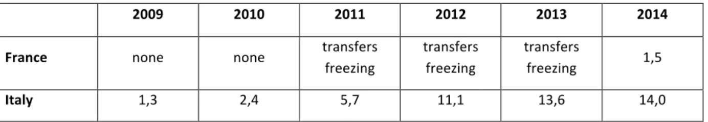
measures the LG intends to punt in place, with the aim to access a special anti-default revolving fund that should be paid back along years. 3.2.1 Italy: State-level austerity policies There are at least two characteristics that differentiate the Italian answer to crisis from the French one, namely its anticipation, since its most severe phase can be dated to 2011 instead of 2014-15 of France, and its complexity. The first symptoms of fiscal crisis arose in 2008, when markets and international institutions, amongst which the EU, started to convey warning signals to the Italian government. Italy then started a series of reforms to strengthen public budgeting, accounting and audit. But the worsening situation also required deep financial cutbacks for municipalities that were obtained via several policies and mechanisms: - Reductions in state grants - Increase of the ISP fiscal targets - Ceilings for specific current expenditures, known as “spending review” policies - Hire freezing The expected overall effects in terms of cutbacks of the policies above can be summarized in Table 2 that also includes the cutbacks operated in France via reduction in state grants, for comparison. Table 2 – Cumulative cutbacks effects on Italian and French municipalities during crisis 2009 2010 2011 2012 2013 2014
France none none transfers
freezing transfers freezing transfers freezing 1,5 Italy 1,3 2,4 5,7 11,1 13,6 14,0 Note: in billion Euros; France – source: ; Italy – source: IFEL 2013.
Coupled with these policies, as said, the central government re-introduced the municipal property tax in 2012 after 4 years of re-centralization of public finances, then in 2013 abolished the property tax on first residences and gave the possibility to raise rates of municipal personal income tax.
4 Methodology
The interaction of the national context and the individual situation in the shaping of LGs’ individual strategies makes it hard to differentiate the influence of each level on the LGs’ resulting financial situation. However, a cross country comparative analysis provides the opportunity to isolate the effects of the national context. Thus, in order to study the influence of both national and individual characteristics, this paper proposes a quantitative comparative study between French and Italian municipalities. Italy and France have a high degree of comparability as they both belong to the Napoleonic administrative tradition group of countries (Ongaro 2010) and to the Euro-zone. Moreover, we chose to study municipalities as they represent the first tier of LGs in both countries.
As a first step of our research, the study focuses on French and Italian municipalities that are over 50 000 inhabitants in 2014, with the exceptions of Paris and Roma that both have a specific institutional profile due to their capital status. In order to catch the effect of the crisis, we use a 11 years’ interval, between 2004 and 2014.
The data collection has been possible thanks to a cooperation with Bureau Van Dijck, Brussels. We have worked on the creation of a database grouping together all financial information available on LGs in France (DIANE PA) and Italy (AIDA PA), and propose scoring, key performance indicators and elements for international comparisons. Unfortunately, some delay in the implementation of the database has forced us to propose here less tests and analysis than what was planned for this paper. After putting aside municipalities for which data was missing, we ended with a sample of 106 municipalities in France and 119 in Italy.
4.1 Selection of variables
As discussed, cross country comparison of municipalities’ financial situation is tricky for several reasons and deserves to be cautious on the choice of variables to study. In order to overcome this first issue, financial data have been reclassified according to recent developments in the field (CEFG Group 2015). The use of the City Economic and Finance Governance group indicators and key performance indicators enables a suitable comparison of French and Italian municipalities’ financial situation as they have faced the comparability and selection issues described above.
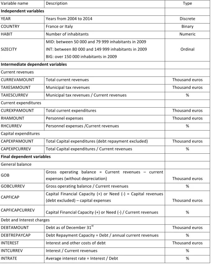
Second issue when comparing financial situation is whether or not using a global scoring. The choice of variables and their weight is always subject to discussion and may lead to controversial results. Moreover, the paper aims at describing the main actions and strategies followed by French and Italian municipalities to balance their budget, in the years following the crisis (cost cuts, downsizing, deferring investment, debt or tax leverage…). So, as a first step of our research, and as an attempt to describe the municipal decisions, we chose to analyze separately the main elements of the municipalities’ financial situation without synthetizing them in one score. As a result of these methodological choices, we studied four groups of dependent variables: current revenues, current expenditures and capital expenditures (our intermediate dependent variables) on one hand, and the financial health in accordance with the main indicators used by the CEFG project (our final dependent variable) on the other. We used several data to operationalize our independent variables. Besides variables for years and for country, to consider the national institutional contexts independent variables, we tried to see if there are differences in the individual strategies implemented to face the crisis, by considering the internal factors independent variables. The expertise of mayors and management teams seems to be greater in bigger municipalities (Kerrouche 2006). Furthermore, there is vast evidence suggesting that the greater an organization is, the more sophisticated management control tools (Anessi-Pessina et al. 2008; Child and Mansfield 1972; Van Dooren 2005). Thus, we use the size of the municipalities measured by number of inhabitants as a proxy for the level of expertise, managerial capacities and the quality of the internal organization. We create a categorical variable that differentiates between middle size cities, intermediary and larger ones. In this first stage of analysis we have not included neither any further internal factors independent variables dimensions, nor any economic and social factors independent variables.
Table 3 provides details for all variables.
Table 3 – List of variables for each municipality
Variable name Description Type
Independent variables
YEAR Years from 2004 to 2014 Discrete
COUNTRY France or Italy Binary
HABIT Number of inhabitants Numeric
SIZECITY MID: between 50 000 and 79 999 inhabitants in 2009 INT: between 80 000 and 149 999 inhabitants in 2009 BIG: over 150 000 inhabitants in 2009 Ordinal Intermediate dependent variables Current revenues
CURREVAMOUNT Total current revenues Thousand euros
TAXESAMOUNT Municipal tax revenues Thousand euros
TAXESCURREV Municipal tax revenues / Current revenues %
Current expenditures
CUREXPAMOUNT Total current expenditures Thousand euros
RHAMOUNT Personnel expenses Thousand euros
RHCURREV Personnel expenses /Current revenues %
Capital expenditures
CAPEXPAMOUNT Total Capital expenditures (debt repayment excluded) Thousand euros
CAPEXPCURREV Total Capital expenditures / Current revenues %
Final dependent variables
General balance
GOB Gross operating balance = Current revenues – current
expenses (without depreciation) Thousand euros
GOBCURREV Gross operating balance / Current revenues %
CAPFICAP Capital Financial Capacity (+) or Need (-) = Capital revenues
(debt excluded) – capital expenses Thousand euros
CAPFICAPCURREV Capital Financial Capacity (+) or Need (-) / Current revenues %
Debt and Interest charges
DEBTAMOUNT Debt as of December 31st Thousand euros
DEBTREPAYCAP Debt Repayment Capacity = Debt / annual current revenues %
INTEREST Interest and other costs of debt Thousand euros
INTCURREV Interest / Current revenues % INTRATE Average interest rate = Interest / Debt %
4.2 Data analysis method
This paper is the first step of a larger research that aims at providing a quantitative overview of the consequences of the crisis and related austerity measures on LGs. Thus, we are here only providing some descriptive statistics and simple linear analysis.To compare the evolution of the French and Italian municipal financial indicators over the years, we draw graphs of the evolution of the average or total amount of each dependent variables between France and Italy over the period. We also use mean comparison tests (t test) to check if differences between France and Italy over the years are significant.
In a second stage, to shed light on the various individual strategies implemented by municipalities to face the crisis, we compare the evolution of the average ratios proposed in table 1, between MID and BIG cities, over the years without differentiating the country they belong to. Thus, we draw graphs and use mean comparison tests (t test) to check if yearly differences are significant.
Before proceeding to tests, we checked the assumptions that underpin the independent t-test.
• Our dependent variables are not normally distributed for each category of the independent variable. But in view of the size of our sample, t-test is considered as a robust test against the normality assumption.
• Our data also failed the hypothesis of homogeneity of variances. Therefore, we used a t-test that does not assume equal variances.
• We monitor the presence of outliers in our data file. Outliers can be due to input errors, indicate the presence in the sample of municipalities with very different behaviors or be the consequence of the limitations of certain measures used. Interpretation of average data are very sensitive to the presence of outliers. It is therefore important to question the decision to keep or delete observations with extreme values. We spotted several extreme values in our samples. They primarily include observations that are not inconsistent with respect to our analysis and so we kept them. However, we had to remove some cases with extreme values that could distort our results, such as the case of Milano for Italy. For variables with outliers, we run all tests with and without extremes values to see if results vary. When the outliers had a too strong influence, we used the sample without outliers. For other variables, we present the results obtained from the full sample. All tests were performed on Stata software.
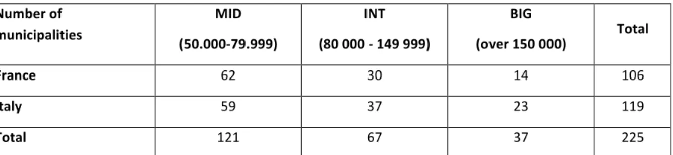
4.3 Sample description
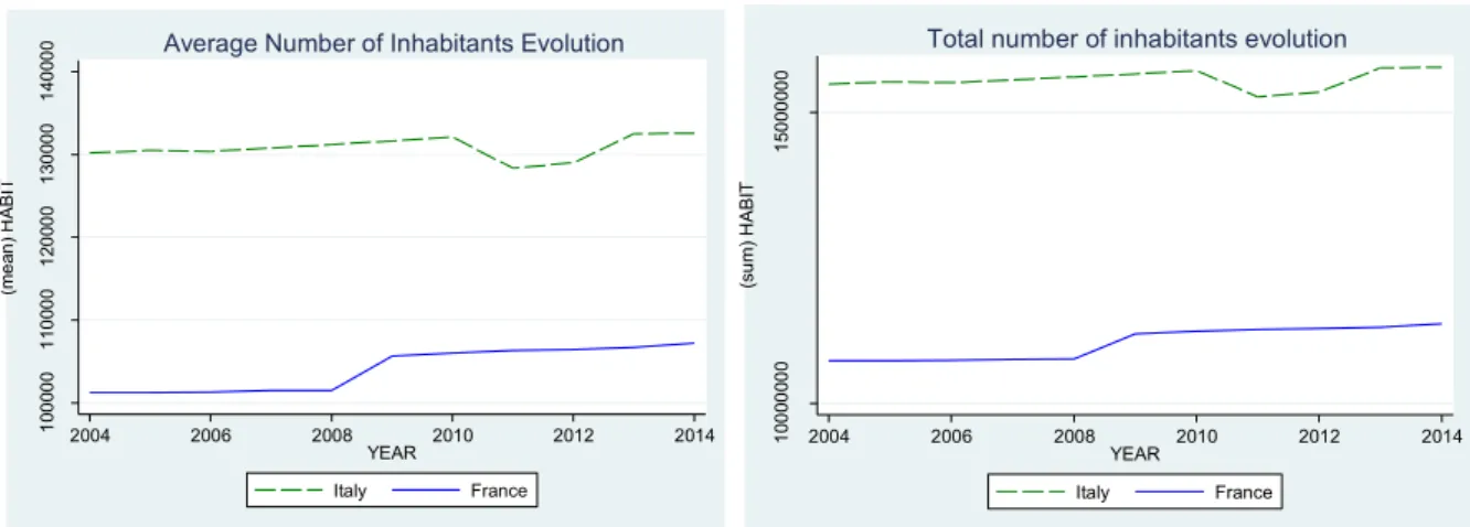
In Table 4 is contained the number of municipalities by dimension. Table 4 - Number of municipalities by size category Number of municipalities MID (50.000-79.999) INT (80 000 - 149 999) BIG (over 150 000) Total France 62 30 14 106 Italy 59 37 23 119 Total 121 67 37 225 Note: MID between 50 000 and 79 999 inhabitants in 2009, INT between 80 000 and 149 999 inhabitants in 2009 , BIG over 150 000 inhabitants in 2009The two graphs below show the evolution of population in France and in Italy, and depending on size, in the sample municipalities. The t-test below shows that even if Italian ones are on average higher, this difference is not significant.
Graph 1 – Number of inhabitants: average and total, in France vs Italy Table 5 - Number of inhabitants: average, in France vs Italy Average number of inhab. 2004 2005 2006 2007 2008 2009 2010 2011 2012 2013 2014 France 101 237 101 237 101 305 101 485 101 506 105 617 105 996 106 309 106 454 106 704 107 210 Italy 130 168 130 500 130 375 130 772 131 198 131 633 132 106 128 331 129 004 132 491 132 567 T-test t(187)=-1,52 t(187)=-1,53 t(188)=-1,53 t(188)=-1,54 t(188)=-1,57 t(194)=-1,35 t(194)=-1,35 t(198)=-1,17 t(197)=-1,19 t(193)=-1,32 t(194)=-1,30 *** (p<0,01), ** (p<0,05), * (p<0,1) Table 6 - Number of inhabitants: average per size category, in France vs Italy Average number of inhab. 2004 2005 2006 2007 2008 2009 2010 2011 2012 2013 2014 MID 58 031 58 107 58 219 58 398 58 623 59 901 60 138 59 745 59 926 60 529 60 661 INT 101 299 101 546 101 628 102 345 102 757 104 613 105 027 103 547 104 000 105 273 105 513 BIG 335 470 335 843 335 118 335 027 334 977 340 612 341 693 334 412 335 581 343 237 344 065 10 00 00 11 00 00 12 00 00 13 00 00 14 00 00 (m e an ) H AB IT 2004 2006 2008 2010 2012 2014 YEAR Italy France
Average Number of Inhabitants Evolution
10 00 00 00 15 00 00 00 (su m) H ABI T 2004 2006 2008 2010 2012 2014 YEAR Italy France
5 Results
5.1 Influence of national context on municipalities’ financial situation throughout the
crisis: a comparison between France and Italy
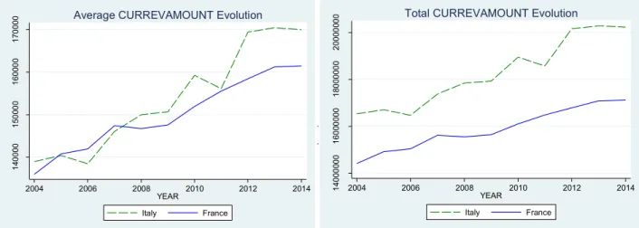
This paragraph presents the results of the comparison between French and Italian municipalities over the years. For each dependent variable, we display a graph of the evolution of average or total (except for ratios) values over years, and per country. We also display a table of the average value with a t-test to check if the differences in means are significant. We color-coded the results: yellow for differences significant at the 1% or 5% level, orange for differences significant at the 10% level, and red for non-significant differences. 5.1.1 Current revenues, current expenditures and capital expenditures: comparative evolution Graph 2 – Current revenues: average and total, France vs Italy Table 7 - Current revenues: average, France vs Italy CURREVAMOU NT 2004 2005 2006 2007 2008 2009 2010 2011 2012 2013 2014 France 135 980 140 752 141 910 147 387 146 747 147 593 151 918 155 525 158 445 161 234 161 483 Italy 138 937 140 413 138 435 146 033 149 982 150 679 159 261 156 121 169 436 170 472 169 985 T-test t(179)=-0,11 t(184)=0,01 t(183)=0,14 t(188)=0,05 t(179)=-0,12 t(178)=-0,12 t(176)=-0,25 t(175)=-0,02 t(157)=-0,31 t(166)=-0,27 t(165)=-0,25 Note: Significant levels *** (p<0,01), ** (p<0,05), * (p<0,1); in thousand euros 14 00 00 15 00 00 16 00 00 17 00 00 (m e an ) C U R R EV AM O U N T 2004 2006 2008 2010 2012 2014 YEAR Italy France Average CURREVAMOUNT Evolution14 00 00 00 16 00 00 00 18 00 00 00 20 00 00 00 (s u m) C U R R EV AM O U N T 2004 2006 2008 2010 2012 2014 YEAR Italy France Total CURREVAMOUNT Evolution
Graph 3 – Municipal taxes: average and total, France vs Italy Note: Sample without outliers Table 8 – Municipal taxes: average, France vs Italy TAXESAMOU NT 2004 2005 2006 2007 2008 2009 2010 2011 2012 2013 2014 France 59 444 61 485 64 196 65 944 67 843 69 874 72 478 74 664 76 871 78 348 79 204 Italy 62 745 63 028 62 111 54 990 46 990 48 065 51 693 71 199 73 057 77 600 82 155 T-test t(186)=-0,34 t(194)=-0,16 t(201)=0,21 t(216)=1,22 t(222)=1,56** t(222)=2,59** t(222)=2,33** t(212)=0,32 t(219)=0,37 t(213)=0,06 t(217)=-0,27 Note: Significant levels *** (p<0,01), ** (p<0,05), * (p<0,1); in thousand euros; sample without outliers Graph 4 – Municipal taxes on current revenues: average, France vs Italy Table 9 - Municipal taxes on current revenues: average, France vs Italy TAXESCURR EV 2004 2005 2006 2007 2008 2009 2010 2011 2012 2013 2014 France 44,7% 44,7% 45,4% 45,3% 46,3% 47,4% 47,4% 47,5% 48,3% 48,6% 49,0% Italy 53,6% 54,2% 54,1% 45,4% 39,0% 38,8% 39,4% 60,8% 63,9% 60,5% 67,9% T-test t(215)=-5,67*** t(213)=-5,92*** t(216)=-5,34*** t(222)=-0,1 t(222)=5,15*** t(222)=6,14*** t(221)=5,99*** t(194)=-7,44*** t(207)=-9,54*** t(218)=-8,3*** 13,53*** t(218)=-Note: Significant levels *** (p<0,01), ** (p<0,05), * (p<0,1) 50 00 0 60 00 0 70 00 0 80 00 0 (me an ) T AXESAMO U N T 2004 2006 2008 2010 2012 2014 YEAR Italy France
Average TAXESAMOUNT Evolution
50 00 00 060 00 00 070 00 00 080 00 00 090 00 00 010 00 00 00 (s u m) T AX ES AM O U N T 2004 2006 2008 2010 2012 2014 YEAR Italy France Total TAXESAMOUNT Evolution
.4 .5 .6 .7 (m e an ) T AX ES C U R R EV 2004 2006 2008 2010 2012 2014 YEAR Italy France
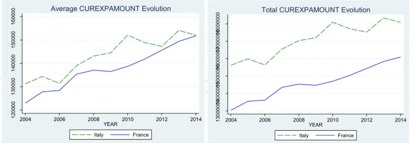
Graph 5 – Current expenditures: average and total, France vs Italy Table 10 – Current expenditures: average, France vs Italy CUREXPAMO UNT 2004 2005 2006 2007 2008 2009 2010 2011 2012 2013 2014 France 122 949 127 815 128 442 135 387 137 101 136 477 138 693 141 831 145 630 149 398 151 836 Italy 131 248 134 382 131 381 139 003 143 135 144 491 152 057 148 885 147 265 154 128 151 975 T-test t(176)=-0,35 t(180)=-0,26 t(178)=-0,12 t(183)=-0,14 t(179)=-0,23 t(173)=-0,31 t(170)=-0,48 t(168)=-0,25 t(170)=-0,06 t(173)=-0,16 t(170)=-0,0 Note: Significant levels *** (p<0,01), ** (p<0,05), * (p<0,1); in thousand euros Graph 6 – Personnel expenditures: average and total, France vs Italy Table 11 – Personnel expenditures: average, France vs Italy RHAMOUN T 2004 2005 2006 2007 2008 2009 2010 2011 2012 2013 2014 France 62 005 64 004 66 258 69 169 71 176 71 580 72 471 73 986 75 434 77 505 80 620 Italy 44 703 45 717 46 833 47 198 48 058 48 049 46 946 45 732 43 403 42 352 41 344 T-test t(213)=1,81* t(214)=1, 88* t(214)=1, 94* t(216)=2, 15** t(217)=2, 22** t(215)=2, 3** t(217)=2, 52** t(220)=2, 8*** t(223)=3, 27*** t(223)=3, 57*** t(222)=3, 95*** Note: Significant levels *** (p<0,01), ** (p<0,05), * (p<0,1); in thousand euros 12 00 00 13 00 00 14 00 00 15 00 00 16 00 00 (m e an ) C U R EX PA MO U N T 2004 2006 2008 2010 2012 2014 YEAR Italy France Average CUREXPAMOUNT Evolution
13 00 00 0014 00 00 0015 00 00 0016 00 00 0017 00 00 0018 00 00 00 (s u m) C U R EX PA MO U N T 2004 2006 2008 2010 2012 2014 YEAR Italy France Total CUREXPAMOUNT Evolution
40 00 0 50 00 0 60 00 0 70 00 0 80 00 0 (m e an ) R H AM O U N T 2004 2006 2008 2010 2012 2014 YEAR Italy France
Average RHAMOUNT Evolution
50 00 00 0 60 00 00 0 70 00 00 0 80 00 00 0 90 00 00 0 (s u m) R H AM O U N T 2004 2006 2008 2010 2012 2014 YEAR Italy France
Graph 7 – Personnel expenditures on current revenues: average, France vs Italy Table 12 - Personnel expenditures on current revenues: average, France vs Italy RHCURREV 2004 2005 2006 2007 2008 2009 2010 2011 2012 2013 2014 France 46% 46% 47% 48% 49% 49% 49% 48% 49% 49% 51% Italy 31% 31% 32% 31% 31% 30% 28% 28% 26% 25% 24% T-test t(221)=1 9,07*** t(218)=9 ,48*** t(222)=1 8,56*** t(221)=2 0,01*** t(221)=2 0,82*** t(217)=2 0,42*** t(222)=2 3,41*** t(216)=2 3,53*** t(211)=2 6,71*** t(203)=3 0,16*** t(191)=3 3,44*** Note: Significant levels *** (p<0,01), ** (p<0,05), * (p<0,1) Graph 8 – Capital expenditures: average and total, France vs Italy Table 13 – Capital expenditures: average, France vs Italy CAPEXPAMOU NT 2004 2005 2006 2007 2008 2009 2010 2011 2012 2013 2014 France 47 325 56 714 49 113 53 470 49 443 52 440 45 012 47 907 51 190 53 652 46 827 Italy 54 352 50 360 36 225 34 676 34 657 28 669 30 522 23 588 20 379 22 959 24 706 T-test t(195)=-0,75 t(217)=0,6 t(222)=1,75 * t(217)=1,96* t(210)=1,91 * t(184)=3,25 *** t(219)=2,32 ** t(220)=3,94 *** t(184)=5,7 *** t(220)=4,35 *** t(195)= 2,8*** Note: Significant levels *** (p<0,01), ** (p<0,05), * (p<0,1); in thousand euros; sample without outliers .2 5 .3 .3 5 .4 .4 5 .5 (m e an ) R H C U R R EV 2004 2006 2008 2010 2012 2014 YEAR Italy France
Average RHCURREV Evolution
20 00 0 30 00 0 40 00 0 50 00 0 60 00 0 (m e an ) C AP EX PA MO U N T 2004 2006 2008 2010 2012 2014 YEAR Italy France
Average CAPEXPAMOUNT Evolution
20 00 00 0 30 00 00 0 40 00 00 0 50 00 00 0 60 00 00 0 (s u m) C AP EX PA MO U N T 2004 2006 2008 2010 2012 2014 YEAR Italy France
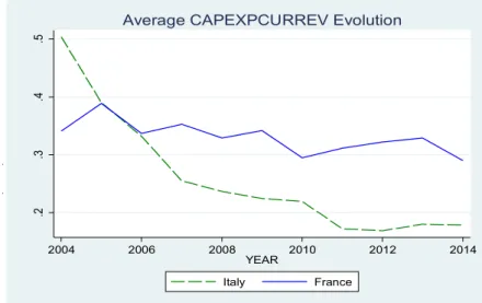
Graph 9 – Capital expenditures on current revenues: average, France vs Italy Table 14 - Capital expenditures on current revenues: average, France vs Italy CAPEXPCUR REV 2004 2005 2006 2007 2008 2009 2010 2011 2012 2013 2014 France 34,1% 38,9% 33,7% 35,3% 32,9% 34,2% 29,5% 31,1% 32,2% 32,9% 29,0% Italy 50,4% 39,0% 33,2% 25,5% 23,7% 22,5% 22,0% 17,2% 16,9% 18,0% 17,9% T-test t(147)=-3,31** t(215)=-0,03 t(218)=0,18 t(223)=4,42*** t(218)=5,54*** t(186)=4,62*** t(215)=4,49*** t(223)=7,58*** t(217)=7,61*** t(147)=3,78*** t(131)=2,15*** Note: Significant levels *** (p<0,01), ** (p<0,05), * (p<0,1) 5.1.2 Financial health: comparative evolution Graph 10 – Gross operating balance: average and total, France vs Italy Table 15 – Gross operating balance: average, France vs Italy GOB 2004 2005 2006 2007 2008 2009 2010 2011 2012 2013 2014 France 18 375 17 524 18 446 17 038 15 085 16 625 19 281 20 303 19 257 18 431 16 162 Italy 6 953 5 147 6 715 7 247 6 907 6 524 7 604 7 369 14 906 12 837 14 495 T-test t(192)=4,77 *** t(152)=6,3 *** t(182)=5,18 *** t(196)=4,27 *** t(212)=3,58 *** t(192)=5,18 *** t(188)=5,19 *** t(171)=5,4 *** t(219)=1,52 t(221)=2,18 t(221)=0,62 Note: Significant levels *** (p<0,01), ** (p<0,05), * (p<0,1); in thousand Euros; sample without outliers .2 .3 .4 .5 (m ea n) C AP EX PC U R R EV 2004 2006 2008 2010 2012 2014 YEAR Italy France
Average CAPEXPCURREV Evolution
50 00 10 00 0 15 00 0 20 00 0 (m e an ) G O B 2004 2006 2008 2010 2012 2014 YEAR Italy France
Average GOB Evolution
50 00 00 10 00 00 0 15 00 00 0 20 00 00 0 25 00 00 0 (s u m) G O B 2004 2006 2008 2010 2012 2014 YEAR Italy France
Graph 11 – Gross operating balance on current revenues: average, France vs Italy Table 16 - Gross operating balance on on current revenues: average, France vs Italy GOBCUR REV 2004 2005 2006 2007 2008 2009 2010 2011 2012 2013 2014 France 12,9% 12,1% 12,4% 10,8% 10,2% 10,7% 12,3% 12,5% 12,1% 11,4% 9,7% Italy 5,1% 4,6% 5,6% 5,3% 3,9% 5,1% 6,0% 5,8% 10,0% 8,5% 10,0% T-test t(223)=10,65 *** t(223)=9,84 *** t(218)=9,7 *** t(215)=5,17 *** t(223)=8,33 *** t(218)=7,51 *** t(221)=9,41 *** t(222)=10,4 6 *** t(223)=3,32 *** t(219)=4,73 *** t(222)=-0,36 Note: Significant levels *** (p<0,01), ** (p<0,05), * (p<0,1) Graph 12 – Capital financial capacity or need: average and total, France vs Italy Table 17 - Capital financial capacity or need: average, France vs Italy CAPFICAP 2004 2005 2006 2007 2008 2009 2010 2011 2012 2013 2014 France 557 -979 -1098 -2369 -1294 -5727 -611 -1774 -1212 -4476 -69 Italy -29231 -21926 -14494 -6885 -8392 -10712 -10353 339 1555 -5162 -7916 T-test t(123)=4,08 *** T(135)=3,3 7 *** t(171)=4,8 4 *** t(174)=2,0 3 ** t(200)=3,3 3 *** t(221)=0,9 4 t(137)=2,4 6 ** t(149)=-0,69 t(203)=-1,43 t(222)=0,25 t(155)=2,2 1 ** Note: Significant levels *** (p<0,01), ** (p<0,05), * (p<0,1); in thousand Euros .0 4 .0 6 .0 8 .1 .1 2 .1 4 (m ea n) G O BC U R R EV 2004 2006 2008 2010 2012 2014 YEAR Italy France
Average GOBCURREV Evolution
-3 00 00 -2 00 00 -1 00 00 0 (m e an ) C AP F IC AP 2004 2006 2008 2010 2012 2014 YEAR Italy France Average CAPFICPAP Evolution
-4 00 00 00 -3 00 00 00 -2 00 00 00 -1 00 00 00 0 (s u m) C AP F IC AP 2004 2006 2008 2010 2012 2014 YEAR Italy France
Graph 13 – Capital financial capacity or need on current revenues: average and total, France vs Italy Table 18 - Capital financial capacity or need on current revenues: average, France vs Italy CAPFICAPCUR REV 2004 2005 2006 2007 2008 2009 2010 2011 2012 2013 2014 France 1,1% -0,5% -1,2% -2,1% -1,5% -2,8% -0,8% -1,4% -1,2% -3,2% -0,1% Italy -19,5% -11,7% -11,9% -4,9% -4,6% -5,4% -4,5% -1,7% -0,3% -1,9% -2,3% T-test t(145)=9,69*** t(194)=8,44*** T(214)=7,77*** t(223)=2,26** t(215)=3,02*** t(146)=1,32 t(222)=4,18*** t(223)=0,39 t(193)=-1,02 t(152)=-1,2 t(200)=1,37** Note: Significant levels *** (p<0,01), ** (p<0,05), * (p<0,1) Graph 14 – Debt: average and total, France vs Italy Table 19 - Debt: average, France vs Italy DEBTAMOU NT 2004 2005 2006 2007 2008 2009 2010 2011 2012 2013 2014 France 103 193 102 970 104 715 107 324 112 793 117 664 118 047 118 225 120 611 123 730 125 996 IT 60 266 64 342 63 777 63 953 63 484 65 523 68 356 67 662 60 408 53 131 72 495 T-test *** *** *** *** *** *** *** *** *** *** *** Note: Significant levels *** (p<0,01), ** (p<0,05), * (p<0,1); in thousand Euros; sample without outliers -.2 -.1 5 -.1 -.0 5 0 (m ea n) C AP FI C AP C U R R EV 2004 2006 2008 2010 2012 2014 YEAR Italy France
Average CAPFICAPCURREV Evolution
60 00 0 80 00 0 10 00 00 12 00 00 14 00 00 (m e an ) D EB T AM O U N T 2004 2006 2008 2010 2012 2014 YEAR Italy France Average DEBTAMOUNT Evolution
60 00 00 0 80 00 00 0 10 00 00 00 12 00 00 00 14 00 00 00 (s u m) D EB T A MO U N T 2004 2006 2008 2010 2012 2014 YEAR Italy France Total DEBTAMOUNT Evolution
Graph 15 – Debt on current revenues: average and total, France vs Italy Table 20 - Debt on current revenues: average, France vs Italy DEBTREPA YCAP 2004 2005 2006 2007 2008 2009 2010 2011 2012 2013 2014 France 84% 82% 82% 82% 85% 86% 85% 84% 85% 85% 86% IT 65% 61% 61% 60% 61% 59% 57% 56% 48% 50% 51% T-test t(216)=3,13*** t(220)=3,69*** t(222)=3,54*** t(223)=3,71*** t(218)=4,10*** t(215)=4,38*** t(212)=4,8*** t(209)=4,77*** t(194)=6,6*** t(219)=6,53*** t(223)=6,39*** Note: Significant levels *** (p<0,01), ** (p<0,05), * (p<0,1); in thousand Euros Graph 16 – Interest expenses: average, France vs Italy Table 21 - Interest expenses: average, France vs Italy INTEREST 2004 2005 2006 2007 2008 2009 2010 2011 2012 2013 2014 France 4715 4496 4792 5108 5430 4953 4307 4685 4725 4811 4972 Italy 6366 6451 6988 7776 8497 7212 6517 6808 6704 6016 6038 T-test t(176)=-1,08 t(175)=-1,31 t(163)=-1,24 t(158)=-1,32 t(156)=-1,38 t(168)=-1,17 t(152)=-1,32 t(152)=-1,2 t(150)=-1,12 t(157)=-0,75 t(153)=-0,62 Note: Significant levels *** (p<0,01), ** (p<0,05), * (p<0,1) 0. 50 00 0. 60 00 0. 70 00 0. 80 00 0. 90 00 (m e an ) D EB T R EP AY C AP 2004 2006 2008 2010 2012 2014 YEAR Italy France
Average DEBTREPAYCAP Evolution
40 00 50 00 60 00 70 00 80 00 90 00 (me an ) IN T ER EST 2004 2006 2008 2010 2012 2014 YEAR Italy France
Graph 17 – Interest expenses on current revenues: average, France vs Italy Table 22 - Interest expenses on current revenues: average, France vs Italy INTCURREV 2004 2005 2006 2007 2008 2009 2010 2011 2012 2013 2014 France 3,4% 3,1% 3,3% 3,4% 3,6% 3,1% 2,8% 3,0% 3,0% 3,1% 3,1% Italy 4,2% 4,2% 4,3% 4,5% 4,7% 4,0% 3,6% 3,7% 3,5% 3,0% 2,9% T-test t(222)=-2,90*** t(217)=-3,92*** t(216)=-3,95*** t(217)=-3,97*** t(216)=-3,66*** t(211)=-2,66*** t(220)=-2,89*** t(223)=-2,51** t(222)=-1,71* t(219)=0,32 t(213)=0,88 Note: Significant levels *** (p<0,01), ** (p<0,05), * (p<0,1) Graph 18 – Interest expenses on debt (rate): average, France vs Italy Table 23 - Interest expenses on debt (rate): average, France vs Italy INTRATE 2004 2005 2006 2007 2008 2009 2010 2011 2012 2013 2014 France 4,0% 3,9% 3,9% 4,3% 4,2% 3,4% 3,2% 3,5% 3,4% 3,6% 3,8% Italy 11,2% 13,7% 15,2% 15,6% 14,3% 11,6% 9,4% 10,6% 13,3% 10,5% 11,2% T-test t(121)=-4,82*** t(121)=-5,27*** t(118)=-4,57*** t(119)=-4,81*** t(119)=-4,84*** t(119)=-4,83*** t(121)=-6,13*** t(120)=-5,88*** t(119)=-5,48*** t(121)=-4,33*** t(125)=-3,07*** Note: Significant levels *** (p<0,01), ** (p<0,05), * (p<0,1) 0. 03 00 0. 03 50 0. 04 00 0. 04 50 0. 05 00 (m e an ) IN T C U R R EV 2004 2006 2008 2010 2012 2014 YEAR Italy France
Average INTCURREV Evolution
0. 00 00 0. 05 00 0. 10 00 0. 15 00 (m e an ) IN T R AT E 2004 2006 2008 2010 2012 2014 YEAR Italy France