A 3D physical model to study the behavior of vegetation fires at laboratory scale

HAL Id: hal-02114685

https://hal-amu.archives-ouvertes.fr/hal-02114685

HAL is a multi-disciplinary open access archive for the deposit and dissemination of sci-entific research documents, whether they are pub-lished or not. The documents may come from teaching and research institutions in France or abroad, or from public or private research centers.

L’archive ouverte pluridisciplinaire HAL, est destinée au dépôt et à la diffusion de documents scientifiques de niveau recherche, publiés ou non, émanant des établissements d’enseignement et de recherche français ou étrangers, des laboratoires publics ou privés.

Dominique Morvan, Gilbert Accary, Sofiane Meradji, Nicolas Frangieh, Oleg

Bessonov

To cite this version:

Dominique Morvan, Gilbert Accary, Sofiane Meradji, Nicolas Frangieh, Oleg Bessonov. A 3D physical model to study the behavior of vegetation fires at laboratory scale. Fire Safety Journal, Elsevier, 2018, 101, pp.39-52. �10.1016/j.firesaf.2018.08.011�. �hal-02114685�

A 3D physical model to study the behavior of vegetation fires at laboratory scale Dominique Morvan, Gilbert Accary, Sofiane Meradji, Nicolas Frangieh, Oleg Bessonov

PII: S0379-7112(18)30022-5

DOI: 10.1016/j.firesaf.2018.08.011

Reference: FISJ 2739

To appear in: Fire Safety Journal

Received Date: 16 January 2018 Revised Date: 13 August 2018 Accepted Date: 16 August 2018

Please cite this article as: D. Morvan, G. Accary, S. Meradji, N. Frangieh, O. Bessonov, A 3D physical model to study the behavior of vegetation fires at laboratory scale, Fire Safety Journal (2018), doi: 10.1016/j.firesaf.2018.08.011.

This is a PDF file of an unedited manuscript that has been accepted for publication. As a service to our customers we are providing this early version of the manuscript. The manuscript will undergo copyediting, typesetting, and review of the resulting proof before it is published in its final form. Please note that during the production process errors may be discovered which could affect the content, and all legal disclaimers that apply to the journal pertain.

M

AN

US

CR

IP

T

AC

CE

PT

ED

A 3D physical model to study the behavior of vegetation fires at

laboratory scale

Dominique Morvan 1*_{, Gilbert Accary} 2_{, Sofiane Meradji} 3_{, Nicolas Frangieh} 1_{, Oleg Bessonov} 4 3

4

1 _{Aix-Marseille University, CNRS, Centrale Marseille, M2P2, Marseille, France}

5

2 _{Scientific Research Center in Engineering, Lebanese University, Lebanon}

6

3 _{IMATH, EA 2134, Toulon University, France}

7

4 _{Institute for Problems in Mechanics RAS, Russia}

8 9

(*) Corresponding author: [email protected]

10 11

Abstract

12

A 3D multi-physical model referred to as “FireStar3D” has been developed in order to

13

predict the behavior of wildfires at a local scale (< 500m). In the continuity of a previous

14

work limited to 2D configurations, this model consists of solving the conservation

15

equations of the coupled system composed of the vegetation and the surrounding gaseous

16

medium. In particular, the model is able to account explicitly for all the mechanisms of

17

degradation of the vegetation (by drying, pyrolysis, and heterogeneous combustion) and

18

the various interactions between the gas mixture (ambient air + pyrolysis and combustion

19

products) and the vegetation cover such as drag force, heat transfer by convection and

20

radiation, and mass transfer. Compared to previous work, some new features were

21

introduced in the modelling of the surface combustion of charcoal, the calculation of the

22

heat transfer coefficient between the solid fuel particles and the surrounding atmosphere,

23

and many improvements were brought to the numerical method to enable affordable 3D

24

simulations. The partial validation of the model was based on some comparisons with

25

experimental data collected at small scale fires carried out in the Missoula Fire Sciences

26

Lab’s wind tunnel, through various solid-fuel layers and in well controlled conditions. A

27

relative good agreement was obtained for most of the simulations that were conducted. A

28

parametric study of the dependence of the rate of spread on the wind speed and on the

29

fuelbed characteristics is presented.

30

Keywords: Forest fuel fire, Detailed physical fire model, Fire physics

31 32

Nomenclature

33

, , ′ Reynolds average, Favre average, and fluctuation of a generic field

34

variable φ

35

CD Drag coefficient of solid particles

36

CS Heat capacity of solid particles

M

AN

US

CR

IP

T

AC

CE

PT

ED

D Diameter of cylindrical solid particles

38

FDi Drag force in direction i resulting from solid particles

39

fv Volume fraction of soot in the gas mixture

40

gi Gravity acceleration in direction i

41

h, hα Enthalpy of the gas mixture and enthalpy of chemical species α

42

hS Heat transfer coefficient between the gas mixture and the solid

43

particles

44

∆hChar,∆hPyr,∆hVap, Charcoal combustion heat, pyrolysis heat, and water vaporization heat

45

I Radiation intensity

46

J Total irradiance

47

k Turbulent kinetic energy

48

Nu Nusselt number of solid particles

49

m Superscript referring to a vegetation family

50

M Vegetation moisture content

51

Mass rate of production of chemical species α resulting from

52

vegetation decomposition

53

P, Pα Pressure of the gas mixture and partial pressure of chemical species α

54

in the mixture

55

Pth, Phs Thermodynamic and hydrostatic pressures of the gas mixture

56

Pr, PrT Laminar and turbulent Prandtl numbers of the gas mixture

57

, _, , _, Rate of heat transferred to the solid particles (total, from solid-fuel

58

combustion, and by convection)

59

R0, Rα Universal ideal gas constant and specific gas constant of chemical

60

species α

61

RaD Rayleigh number of cylindrical solid particles

62

ReD Reynolds number of cylindrical solid particles

63

ReT Turbulent Reynolds number

64

ROS Rate of spread of fire

65

Sc Schmidt number of chemical species

66

t Time

67

T, T_S Temperature of the gas mixture and of the solid particles

68

U Wind speed at wind tunnel entrance

69

ui Velocity vector component in direction i

70

xi Cartesian coordinate in direction i

71

Yα Mass fraction of chemical specie α in the gas mixture

72

YAsh, YChar, YDry, YH2O Mass fraction of ash, charcoal, dry material, and water in solid

73

particles

74

Greek symbol

M

AN

US

CR

IP

T

AC

CE

PT

ED

αG, αS Volume fraction of the gaseous phase and of the solid phase

76

αSG Fraction of combustion heat absorbed by solid particles

77

δ Fuel bed depth

78

δij Kronecker coefficient

79

ε Dissipation of turbulent kinetic energy

80

ϕ Multiplying factor of S O2

ν depending on the molar ratio of CO to CO2 81

gases produced from charcoal combustion

82

λ Thermal conductivity of the gas mixture

83

µ, µT, µe Dynamic viscosity, turbulent viscosity, and effective viscosity of the

84

gas mixture

85

νChar, νSoot, νCO2, νAsh Mass fraction of charcoal, soot, CO2 gas, and ash resulting from the 86

pyrolysis of dry material

87

, , Mass stoichiometric coefficient of charcoal, CO, and soot combustion

88

, , Rate of charcoal combustion, of dry material pyrolysis, and of water

89

vaporization in solid particles

90

Rate of production of chemical species α resulting from reaction in the

91

gaseous phase

92

ρ, ρDry, ρS, ρSoot, Density of the gaseous phase, of dry material, of the solid phase, of

93

soot, and of solid-fuel elements

94

σ Stephan-Boltzmann constant

95

σS Surface area-to-volume ratio of the solid particles

96

σG Absorption coefficient of the gas/soot mixture

97

τopt Fuel-bed optical thickness

98 99

1. Introduction

100

In a near future, numerous factors such as global warming, extensive urbanization, and

101

reduction of agriculture activities could potentially contribute to increase fire hazard in

102

many regions worldwide [1]. However, in adopting the fire ecology point of view [2],

103

wildfires cannot always be considered as a natural disaster, in many cases they contribute

104

to maintain the ecological equilibrium of an ecosystem and help the renewal of forests (in

105

eliminating old trees and promoting, after the fire, the growth of new young trees). The

106

relationship between fires and ecosystems can be summarized by the fire regime, which

107

integrates various characteristics of fire and is generally summarized as the observed

108

average frequency between two fires. A modification of the fire regime, especially if it

109

appears in a short time, is an indication of a perturbation in the life of an ecosystem due to

110

human activities and an evolution of the climate. In this context, if a fire is ignited in a wild

111

ecosystem, the better response could be to do nothing, considering that the perturbation

112

induced by this fire is necessary to maintain a certain equilibrium. However, this approach

M

AN

US

CR

IP

T

AC

CE

PT

ED

reaches its own limits if the fire affects urban structures such as housing developments in

114

what is commonly referred as the Wildland−Urban Interface (WUI) [3]. The reduction of

115

this natural hazard needs a better understanding of the physical mechanisms governing the

116

behavior of a fire during different phases (ignition, propagation, and extinction), the role

117

played by various parameters characterizing the structure and the state of the vegetation,

118

but also the effects of external conditions such as the wind, air temperature and humidity,

119

the topography, and many other factors. The development of new fire safety engineering

120

tools, based on numerical simulations will allow, in the near future, for the ability to predict

121

the trajectory of a fire front through a landscape (at large scale) or to describe in more

122

details the interaction at a smaller scale between the flames and potential targets located

123

inside the WUI ( e.g., vegetation, houses, etc.) [4,5].

124

As highlighted in the literature, most of the operational tools developed in order to predict

125

the propagation of a fire front at a landscape scale are based on statistical or

semi-126

empirical approaches [6]. Unfortunately, the use of this class of models under conditions

127

that deviate from those used to construct the database, can lead to unacceptable failures;

128

for example, in some cases, the rate of spread of the fire can exceed the wind speed (wind

129

speed measured at a sufficient height 10m open wind speed), which is totally unphysical

130

except if the wind speed tends to zero. This has motivated the development of a new class

131

of models, based on a “fully” physical approach, for which the rate of fire spread, and more

132

generally, all variables (flame geometry, fire intensity, etc.) characterizing fire behavior are

133

addressed through the resolution of balance equations governing the various interactions

134

occurring between the vegetation, the surrounding atmosphere, and the flame [5]. The

135

multiphase approach, initially introduced by A.M. Grishin in a monograph at the end of 90’s

136

[7], is based on a very detailed modeling of the physicochemical phenomena involved in a

137

fire, from the thermal degradation of the vegetation to the development of the turbulent

138

flame inside and above the vegetation layer. The model developed in this work, referred to

139

as “FireStar3D”, can be considered to belong to this multiphase class of models. Globally,

140

this approach solves two sets of problems, one for the vegetation and one for the

141

surrounding gas. These two sets of problems are coupled through additional terms in the

142

balance equations (mass, momentum, and energy) governing the physical system. No

143

modeling of the interface between the solid phase and the gaseous one was introduced in

144

the model, the geometrical complexity (fractal in nature) does not permit an easy

145

description of this interface. In an approach similar to that used to describe fluid flow in a

146

porous medium, the equations were averaged in a representative elementary volume

147

including the two phases. This preliminary operation is responsible for the introduction of

148

additional source terms in the average balance equations (gas production due to pyrolysis,

149

drag force, convection and radiation heat exchange with the solid phase). Except for some

150

particular cases clearly indicated in the text, all the constants of the different sub-models

151

have been fixed from experimental data referenced in Grishin's monograph [7]. Of course,

M

AN

US

CR

IP

T

AC

CE

PT

ED

the value of these constants are the same for all the reported simulations. Because this kind

153

of model includes a high level of details in representing a propagating fire front and its use

154

is limited to describe the behavior of a fire at a relatively local scale (few hundred meters),

155

which is compatible with the study of the interaction between a wildfire and a house or a

156

building. A very close version of this model is already operational in a 2D approximation

157

[8–10] , in this case, the problem is solved in a vertical plane defined by the direction of

158

propagation of fire. The 3D extension of the existing model enables to render the 3D effects

159

observed in real fires [11] and to represent the real heterogeneous structure of the

160

vegetation both near the surface (for the shrubs) and the canopy (trees). The main

161

difference between 2D and 3D simulations is that in 2D the fire front is assumed to form a

162

homogeneous obstacle forcing the inlet wind flow to be deviated vertically with the

163

convective plume. In 3D, the heterogeneity of the fire front, forming a succession of peaks

164

and valleys, oscillating under the action of a thermo-convective instability, allows the inlet

165

wind flow to cross the fire front. This difference of behavior of the fire front, contributes to

166

modification of the trajectory of the flame, and also of the plume, and consequently, it

167

greatly affects the interaction between the fire front and the vegetation layer. The

168

difference in behavior between 2D and 3D simulated fires have been investigated by Linn

169

et al. [11] using the coupled atmosphere-fire model HIGRAD/FIRETEC. Even in simulating a

170

quasi-infinite fire front in 3D, using cyclic conditions in the horizontal direction

171

perpendicular to the direction of propagation, the numerical results have highlighted how

172

3D effects can affect the propagation of the fire, and particularly the relationship rate of

173

spread versus wind speed.

174

The present paper has two main objectives: (i) to present some details of the 3D model and

175

(ii) to evaluate the potential of the model in predicting the rate of fire spread in

well-176

controlled experimental conditions such as the surface fire performed in the wind-tunnel of

177

the Missoula Fire Sciences Lab [12]. One of the main interests in considering the

178

experiments carried out at Missoula Laboratory was that they had been conducted with a

179

significant number of varieties of fuel particles (pines needles, excelsior, sticks) covering a

180

large range of the solid fuel parameters, such as the surface area to volume ratio, the

181

packing ratio, and the moisture content. Before tackling the problem at large scale, for

182

example, simulating grassland fire experiments carried out in Australia or in US [13,14],

183

this paper represents a first step in evaluating the numerical results obtained with our 3D

184

model to experimental laboratory-scale data collected under well-controlled conditions.

185 186

2. Mathematical Model

187

The mathematical model of FireStar3D consists of two main parts, coupled through

188

interaction terms. The first part is devoted to the evolution of the state of the vegetation

189

subjected to the intense heat flux coming from the flaming zone. The second part is devoted

M

AN

US

CR

IP

T

AC

CE

PT

ED

to the calculation of the turbulent-reactive gas flow resulting from the mixture of the

191

pyrolysis and combustion products with the ambient air.

192

Firestar3D includes most of the characteristics already integrated in the previous 2D

193

version, i.e. a volume decomposition model to represent the different steps of degradation

194

of the vegetation (drying, pyrolysis, char oxidation), a non-equilibrium multiphase model

195

to represent all the fine fuel elements constituting a vegetation layer (foliage, twigs of

196

various diameters), a low Mach number implicit Navier-Stokes solver including a turbulent

197

combustion model in the gaseous phase, and a multiphase model to represent the radiation

198

heat transfer coming both from the gas species (H2O, CO, CO2 …) and the soot [8–10]. 199

Particular attention was focused on the quality of the numerical convection scheme used

200

for the resolution of the transport equations in the gaseous phase, in order to avoid

201

numerical diffusion (this is capital for turbulence modeling), as well as to the

202

parallelization of the code in order to enable affordable 3D simulations. These

203

characteristics, which can contribute to the future potential of this tool, cannot all be found

204

in the other 3D wildfire models available in the community, such as FIRETEC and WFDS

205

[15–17]. Many of these well-known tools [16,17] use an explicit solver for the resolution of

206

the Navier-Stokes equations; such solvers are usually used to simulate fully compressible

207

flows, which is not the best approach for the simulation of low Mach number flows, mainly

208

because of a wide disparity between the time scales associated with convection and the

209

propagation of acoustic waves [18]. To guarantee the stability of the numerical schemes in

210

the case of fully compressible solvers, the time step and the mesh size must verify

Courant-211

Friedrich stability criterion based on the maximum value between the speed of sound and

212

the gas flow velocity. Under the low Mach number approximation, the same criterion is

213

only based on the gas flow velocity. For low Mach number flows, this constitutes a great

214

difference (if one is not interested in the propagation of acoustic waves) since the time step

215

can be easily multiplied by a factor ranged between 10 and 100 (depending the robustness

216

of the convection scheme) without any loss of accuracy in the description of the

217

phenomena of interest. In summary, choosing a fully compressible formulation and an

218

associated explicit solver, as in FIRETEC for example, constitutes a major limitation

219

especially to simulate wildfire at large scale. This is the main reason behind the mesh size

220

used in FIRETEC that can reach, for example, one meter high at ground level, exceeding

221

sometimes the height of the fuel layer, with the consequence that the pyrolysis process and

222

the heat release due to the combustion within the entire fuel layer thickness take place

223

inside one and the same computational cell. In addition, other physical aspects (turbulent

224

combustion, radiation heat transfer, soot production and transport …) are not well

225

described in WFDS and FIRETEC, especially within the fuel layer. An overview of the

226

discrepancies between these different “fully” physical fire-models can be found in reference

227

[15], summarized also in Tab. 1.

M

AN

US

CR

IP

T

AC

CE

PT

ED

As indicated in the introduction, some new features have been added in FireStar3D, such as

229

the process of charcoal combustion and the evaluation of the heat transfer coefficient

230

between the solid phase and the gaseous one. These new features are presented in the

231 following parts. 232 233 234 235

FireStar2D FireStar3D WFDS FIRETECH FIREFOAM Solver 2D-Implicit 3D-Implicit 3D-Explicit 3D-Explicit 3D-Implicit

Low Mach model Yes Yes Yes No Yes(1)

Turbulence TRANS TRANS/LES LES LES LES

TRI model Yes No Yes(2) _Yes(2) _No

Combustion model Yes Yes Yes No(3) _Yes

Multi-fuel model Yes Yes Yes Yes No

Small scale Yes Yes Yes No Yes

Large scale Yes(4) _{Yes Yes Yes Yes}

236

Tab. 1. Summary of main characteristics of four fully physical fire models. (1) _{Work in}

progress. (2) _{The radiation heat transfer was increased empirically.} (3)

Pyrolysis and combustion take place at the same location without transport into the gaseous phase. (4) _{With the limitation introduced by the 2D}

assumption.

237

2.1. Solid-Fuel Model

238

The heterogeneous character of the vegetation accounted for using two possible

shape-239

families of solid fuel particles: cylindrical particles (used to represent branches, twigs, and

240

needles), and disks (used to represent flat leaves). At all steps of the decomposition

241

process, each solid fuel family m is characterized using a set of physical variables: the

242

volume fraction (αS), the dry material density (ρDry), the moisture content (M),the surface

243

area-to-volume ratio (σS), the temperature (TS), and the evolution of the composition of

244

fuel particles in terms of mass fraction of char, water and dry fuel. Measurements of the fire

245

residence time measured for homogeneous solid-fuel beds in laboratory [19], have shown

246

that only small fuel particles (σS > 600 m-1 corresponding to a diameter D < 6 mm for

247

cylindrical shape particles) can contribute actively to the dynamics of a fire. This result was

248

confirmed by wildfire observations, showing that about 90% of thin fuel particles (D < 6

249

mm) were consumed in the flaming zone [20]. This threshold represents also the limit

250

separating the thermally thick and thermally thin particles, which means that the

251

temperature gradient inside each solid fuel particles can be neglected in a first

252

approximation. Thermal analysis of forest fuel samples has highlighted that this kind of

253

material were composed of a mixing of lignin, cellulose, hemicellulose, and extractives [21].

M

AN

US

CR

IP

T

AC

CE

PT

ED

The composition between these various chemical compounds varies from one species to

255

another and between different parts of a plant (bark, branch, twigs, and foliage). At

256

relatively small heating rate (such as the conditions used in thermogravimetric analysis),

257

the chemical composition of fuel particles can affect the dynamics of thermal

258

decomposition, but at higher heating rate (such as the intense heat flux coming from the

259

flaming zone) the result are less sensitive to chemical composition [21] and seems to be

260

more affected by other parameters such as the surface area-to-volume ratio and the fuel

261

moisture content [22, 24]. For these reasons, we consider: (i) that the decomposition of

262

each vegetation family (regardless its composition) can be summarized in three main steps:

263

dehydration, pyrolysis (in only one step), and surface oxidation, (ii) that each family

264

consists locally of a mixture of water, dry material (cellulose, hemicellulose, and lignin),

265

char, and ash (mineral residue). These components are represented by their mass

266

fractions: YH2O, YDry, YChar, and YAsh respectively, resulting in a local density ρS of the

solid-267

fuel.

268

The fuel model consists of decomposing the fuelbed zone into homogeneous

solid-269

fuel element of effective density = . It is assumed that the pyrolysis process would

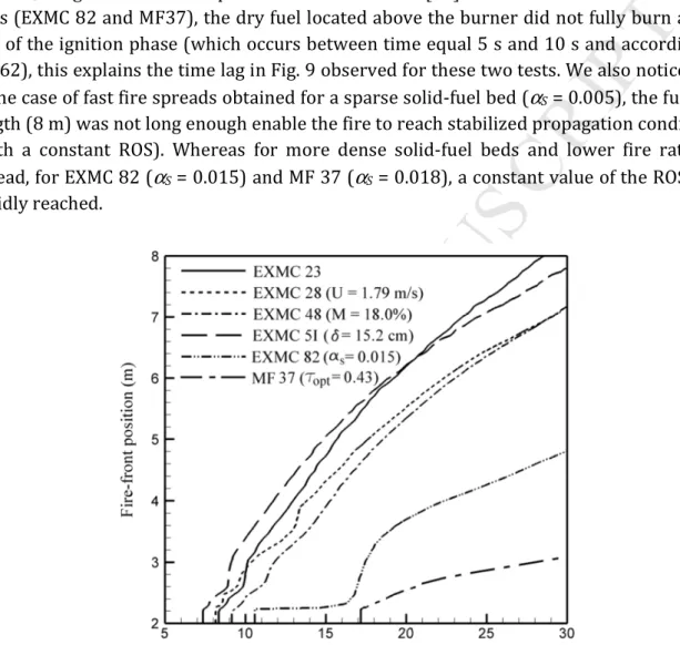
270

be activated only if the dehydration was entirely completed, and that surface oxidation

271

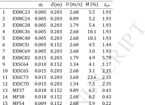
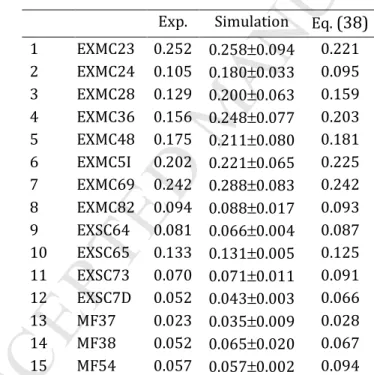
would begin only if the pyrolysis process came to an end.

272

In the dehydration phase, the evapotranspiration process is reduced to a simple

273

vaporization, during which the temperature of the solid fuel element TS is assumed to

274

remain constant at 373K. The rate of heat transfer received by that fuel element from

275

the flaming zone only serves to produce water vapor at the mass rate:

276 277

= ! = $∆ℎ (1) 278

279

where ∆hVap = 2.25×103 kJ/kg is the heat of vaporization.

280

The decomposition of dry combustible by pyrolysis produces gaseous products (CO and

281

CO2) and charcoal. The decomposition of 1 kg of dry combustible is assumed to produce 282

νChar = 0.338 kg of carbon (0.288 kg of charcoal and 0.05 kg of soot), νCO2 = 0.2 kg of CO2 and 283

1 - νChar - νCO2 = 0.462 kg of CO. By contact with the oxygen contained in the ambient air, the

284

hot combustible pyrolysis-products (CO and soot) ignite homogeneously in the gaseous

285

phase. Taking into account these assumptions, the pyrolysis process obeys to the following

286

transformation equation written for 1kg of dry combustible:

287

(

)

(

)

combustibe

Dry → ν_Char −ν_Soot +ν_Soot +ν_{CO2 2}+ 1−ν_Char −ν_{CO2 (1)}

The pyrolysis process is assumed to take place when the solid fuel element TS is between

288

400K and 500K [8, 19, 21] at the mass rate:

289 290

M

AN

US

CR

IP

T

AC

CE

PT

ED

where ∆hPyr is the pyrolysis heat that depend on the vegetation species. We can notice that

292

this range of temperature values is slightly lower than the range 473-573 K found in [21].

293

This discrepancy can be explained by a scale effect: in the present study, the solid-fuel

294

temperature represents an average value evaluated within a 1 cm3 _{volume (with a} 295

temperature gradient reported in [21]), whereas the temperature reported in [21] was

296

measured with a 0.5 mm thermocouple. In addition, this temperature range [400-500 K]

297

has allowed us to obtain the best results in comparison with experimental data obtained at

298

the same scale and comparable solid fuel [25] (see also Fig. 1 in reference [8]). Thus

299

according to Eq. 3, a portion of the rate of heat transfer received by the fuel element

300

contributes to the pyrolysis process, while the remaining portion of continues to

301

increase the solid fuel temperature TS. Note that TS cannot exceed 500K as long as the

302

pyrolysis process has not ended.

303

Unlike previous works [8–10] that arbitrary assumed a complete combustion of charcoal

304

(thus producing only CO2) at the solid-fuel particles, in the present work the model 305

representing the surface oxidation of charcoal has been modified to account for a possible

306

incomplete combustion, thus producing both CO and CO2. According to [23], the balance 307

equation written for 1kg of charcoal is given by:

308

(

)

(

)

(

)

(

)

2

2 O 2 1 CO 1 2 1 CO

C +ν_OS ϕ → +ν_OS −ϕ + +ν_OS ϕ − (2) where = 8/3 and ϕ is the mass stoichiometric coefficient, it depends on the molar

309

ratio of CO to CO2 gases produced from charcoal combustion and is given by: 310 2 2 2 2 2 + × + = CO CO CO CO

ϕ

The molar ratio of CO to CO2 gases depends on the surface temperature TS according to the

311 following relation [23]: 312

(

)

At low temperatures, ϕ→ 1 and only CO2 is produced, while at high temperatures, ϕ→ 0.5 313

and only CO is practically produced.

314

The reaction rate of charcoal combustion is approximated by the following Arrhenius law:

315 316

= + , -./0−1 /34& 5 6 (7) 317

318

where PO2 is the partial pressure of O2 at the solid fuel particle surface. The frequency 319

factors kChar = 254.2 kg/(m2.s.atm) and activation energy EChar/R0 = 9000K are evaluated

320

experimentally from a thermal analysis [23].

M

AN

US

CR

IP

T

AC

CE

PT

ED

Heat released during charcoal combustion, taking place at the surface of a solid-fuel

322

particle, is assumed to be absorbed both by the solid-fuel element and by the gaseous

323

phase. The rate of heat absorbed by the solid-fuel element is calculated as follows:

324 325

, = ∆ℎ (8)

326 327

where ∆hChar is the combustion heat given by:

328

(

)

(

)

(

)

(

)

with ∆hCO = 9 MJ/kg and ∆hCO2 = 30 MJ/kg are the reaction heats of incomplete and

329

complete combustion of carbon that can be obtained from Eq. (2) by setting ϕ at 0.5 and 1

330

respectively. We assume in this study that heat released during charcoal combustion is

331

equally shared by the gaseous phase and by the solid-fuel element, i.e. αSG = 0.5.

332

Taking into account all the previous equations and assumptions, time evolution of the

333

composition and the temperature of a family m of solid-fuel particles in the fuelbed are

334

controlled by the following set of six equations [8–10]:

335 336 7 78 0 9 9 :!9 5 = − (10) 337 7 78 ; 9 9 :<9 = = − (11) 338 7 78 0 9 9 :9 5 = 0 − 5 − >1 + AB C (12) 339 340 7 78 0 9 95 = − − 01 − + 5 − (13) 341 7 78 0 9 5 = − 19 (14) 342 9 9 _D97&9 78 = 9 − ∆ℎ − ∆ℎ + ∆ℎ (15) 343

M

AN

US

CR

IP

T

AC

CE

PT

ED

The heat capacity m S

C characterizing locally each solid-fuel element is obtained from a mass

344

fraction-weighted linear combination of the heat capacities of water, dry material, charcoal,

345

and ash. νAsh = 0.033 is the mass fraction of ash in the solid fuel.

346

The rate of heat transfer received by a solid-fuel element results from convection and

347

radiation heat exchanges with the hot gases and is given by [8–10]:

348 349

= ℎ 6 0& − & 5 + 6 0E − 4 6 &F_5/4

(16)

350

where T is the temperature of the gas mixture at the surface of the solid fuel element, σ =

351

5.67×10-8 _W/m2_.K4 _{is the Stephan-Boltzmann constant, and J is the total irradiance (fuel} 352

particles are assumed to behave as a black body). The convection heat transfer coefficient

353

hS depends on the shape of the fuel particles and their characteristic length. For example,

354

for a vegetation family with cylindrical shape particles, hS is obtained from:

355 λ D h Nu= S (6) where Nu is Nusselt number based of the diameter D of a cylindrical solid-particle, and λ is

356

the thermal conductivity of the gas mixture. Unlike previous works [8–10] that only

357

accounted for forced convection, the Nusselt number in the present study accounts for both

358

forced and natural convection and is given by:

359

(

)

where NuFC and NuNC are respectively the forced convection and natural convection Nusselt

360

numbers. NuFC and NuNC are correlated to Prandtl number Pr of the gas mixture and to the

361

Reynolds number ReD and to the Rayleigh number RaD based on the diameter D of a

362

cylindrical solid-particle as follows [26]:

363

(

)

Similar expressions are used to evaluate the convection heat transfer coefficient hS for flat

364

solid-fuel particles.

365

2.2. Gas-Phase Model

366

The evolution of the state of the gaseous phase (composition, velocity, temperature …)

367

resulting from the thermal degradation of the vegetation and the combustion reactions is

368

governed by the balance equations of mass, momentum, and energy. Since the flow regime

M

AN

US

CR

IP

T

AC

CE

PT

ED

is unsteady and fully turbulent in various regions of the computation domain, the equations

370

are filtered using a mass-weighted average TRANS (Favre) formulation [27]. Hence, the

371

filtered variables are governed by the following set of transport equations solved in the low

372

Mach number approximation [18, 28]:

373 374 375 G ̅ G8 = I I₉ 9 (21) 376 377 G0 ̅JKL5 G8 = −M.M,L+ M M.NOP̅ Q MJKL M.N+ MJKN M.L − 2 3MJKM.TTULNVW − M M.N; JXYJZY= + 0 − 45[L− I \<L 9 9 (22) 378 379 G; ̅ℎ= G8 = −M,M8 +M.MNO P̅ ,]M.M&NW − M M.N; JXYℎ Y _{= + 01 − 5∆ℎ I} 9 380 + I I 9_{ℎ + I} , 9 _{+ 6 ;E − 46&}F₌ 9 9 (23) 381 382 G; ̅: = G8 =M.MN^ P̅ _`M:aM.Nb − M M.N; JXY: ′= + + I 9 9 (24) 383

In these equations, all transported variables φ (density ρ, velocity components ui, enthalpy

384

h, and mass fractions Yα of chemical species α : CO, O2, CO2, H2O, and N2) are decomposed as 385

a sum of two contributions (Reynolds average + fluctuation: = + ′). On the other

386

hand, Favre average is defined by: = / ̅. The differential operator D/Dt is defined as:

387

( )

The effective gas-phase density is defined as ρ = αGρG, where ρG is the density of the

gas-388

mixture and αG is the volume fraction of the gaseous given by:

389

∑

−

=

α

α

1

where 9is the volume fraction of family m of solid-fuel particles. ρ0 is the initial gas-phase

390

density that is stratified due to gravity, gi being gravity component in xi direction.

M

AN

US

CR

IP

T

AC

CE

PT

ED

In the low Mach number approximation [18, 28], the acoustic filtering results in splitting

392

the pressure of the gas-mixture, into three contributions: the dynamic pressure P acting to

393

balance inertial and external forces, the thermodynamic pressure Pth that is spatially

394

homogeneous, and the hydrostatic pressure Phs that is time-independent and balances the

395

initial density stratification.

396

In addition to the previous equations, the gas mixture is assumed to behave like an ideal

397

gas. Hence, in low Mach number approximation, the gas-phase density is obtained from the

398

following equation of state:

399 T~ Y~ R P P_{th hs }      = +

∑

where Rα (J/kg.K) is the ideal gas constant of chemical species α (universal gas constant

400

divided by the molar mass).

401

The gaseous phase is assumed also to behave as a Newtonian fluid with a viscosity µ = αGµG,

402

where µG is the dynamic viscosity of the gas mixture obtained from those of the chemical

403

species (µα) using a mass fraction-weighted linear combination. The dependence of µα on

404

temperature is governed by Sutherland law:

405       + +         = S T S T T T~ ref 5 . 1 ref ref α α µ µ ₍₁₃₎

where Tref = 273K, S = 110.4K, and P c is the dynamic viscosities of the chemical species α

406

at temperature Tref. As for dry air in standard conditions, Prandtl and Schmidt numbers are

407

both set to 0.71.

408

The term \_<L9 denotes the ith _{component of the drag force resulting from the dynamic} 409

interaction between the gas flow and the vegetation family m, it is given by:

410 L D i Di

u

~

u

~

C

a

F

=

ρ

where d_e = 6 /2 is the leaves area density and CD is the drag coefficient obtained from

411

correlations that depend on the particles shape of the vegetation family m and on the

412

Reynolds number based on the characteristic length of solid particles [26]. For example, for

413

a vegetation family with cylindrical particles (twigs, needles), the evolution of the drag

414

coefficient with Reynolds number based on the diameter D of the particle is given by:

415 5 0 93 5 17 1 _. D D Re . . C = + ₍₁₅₎

Similar expressions are used to evaluate the drag coefficient CD for flat solid-fuel particles

416

such as leaves.

417

The enthalpy h of the gas mixture is obtained from a mass fraction-weighted linear

418

combination of the enthalpies hα of the chemical species (CO, O2, CO2, H2O, and N2). For 419

each chemical species, the enthalpy-temperature dependence is obtained from CHEMKIN

420

thermodynamic data base [29]:

421

∑

M

AN

US

CR

IP

T

AC

CE

PT

ED

The term 9_, is the average rate of heat exchange by convection between the gas

422

mixture and the solid-fuel family m, obtained from Eq. Error! Reference source not

423

found.. σG is the radiation absorption coefficient of the gas-soot mixture (including the

424

absorption due to the presence of CO, CO2, H2O, and soot particles in the flame and the 425

plumes [30]).

426

During the thermal decomposition of each solid-fuel family m, O2 gas is consumed, CO, CO2, 427

and H2O gases, and charcoal soot particles are produced at the following mass flow rates: 428 429 = − 430 (32) 431 = 01 − − 5 + 02 + 5 01 − f5 (33) 432 = + 01 + 5 02f − 15 (34) 433 ! = (35) 434 = (36) 435

These rates contribute to the source terms of the balance equations of mass, energy and

436

chemical species. Finally, g is the rate of production or destruction of the chemical species

437

α resulting from combustion in the gaseous phase, this part is detailed in the combustion

438 modeling section. 439 440 2.3. Turbulence Modeling 441

The double correlations representing the action of the fluctuations on the average

442

transport equations are evaluated using the eddy viscosity concept [31] and generalized

443

gradient diffusion of the scalar quantities φ as follows:

444 ij l l T i j j i T j i k x u~ 3 2 x u ~ x u~ u u µ µ ρ δ ρ _      + ∂ ∂ −         ∂ ∂ + ∂ ∂ = ′ ′ − ₍₁₇₎ i T i x ~ Pr u ∂ ∂ = ′ ′ −ρ φ µ φ φ ₍₁₈₎

The turbulent viscosity µT is evaluated from the turbulent kinetic energy k and its

445

dissipation rate ε, and an adapted version of RNG-k-ε turbulence model in a high Reynolds

446

number formulation is used [32].

447 ε ρ μ μ μ 2 k C f T = (19)

where Cµ = 0.085 and fµ is a damping function given by Eq. (40) that accounts for

low-448

Reynolds-number effects and allows for a better handling of laminar flow regions.

449

( )

(

)

50

1

4

3

+

−

=

.

Re

f

ln

M

AN

US

CR

IP

T

AC

CE

PT

ED

3-h = ̅+ /Pi is the turbulent Reynolds number. In the limit of a high Reynolds number 450

(µ/µT << 1), Equations (19) and (20) result in: P_h= ̅D_j+ /i.

451

The fields of the turbulent kinetic energy k and its dissipation rate ε are calculated from the

452

two following transport equations:

453

( )

₍

₎

_∑

( )

₍

₎

∑

α

σ

ε

ε

ρ

τ

ε

ρ

τ

τ

ε

µ

ε

ρ

The effective viscosity P = P_h+ P̅, Pk and Wk are respectively the terms contributing to the

454

production of turbulence, due to shear and buoyancy effects [31], given by:

455 j i j i k x u~ u u P ∂ ∂ ′ ′ − = ρ and _j j T T k g x Pr W ∂ ∂ − = ρ ρ μ (23) The effective Prandtl number is computed by iteration using Eq. (24) derived analytically in

456

the RNG theory, where Pr0 = 1 for Pr = PrT, and Pr0 =Pr = Sc for Pr = Prφ.

457 e . . . Pr . Pr . Pr . Pr µ µ = + + − − − − − − 03679 1 0 1 6321 0 1 0 1 3929 2 3929 2 3929 1 3929 1 (24)

In Eq. (41) and (42), the terms proportional to the drag coefficient m D

C represent the

458

production and destruction of turbulence resulting from the interaction between the

459

boundary layer flow and the vegetation layer [33].

460

In the transport equation of ε, τ is the maximum between the integral turbulence time scale

461

(k/ε) and 6τη, where k_l = 0P̅/ ̅i5m/ is the Kolmogorov time scale. This treatment ensures

462

that the time scale associated to the more powerful turbulent structures cannot be smaller

463

than 6 times the turbulence dissipation scales.

464

The additional source term R in the transport equation of ε results from the RNG theory

465

[32] and has extended the validity of this model to weak turbulent flow regions, i.e. near a

466

wall or in the wake region, where turbulence is far from isotropic or homogeneous.

467

(

)

( )

1

1

η

η

βη

η

−

+

=

C

R

where η= ;,_n/D_j ̅i=m/ , η0 = 4.38 and β = 0.012.

468

The following set of constants is introduced in the turbulence model [31]: C1ε = 1.42 and

469

C2ε = 1.68. On the other hand, the degree to which ε is affected by buoyancy is determined

470

by the constant C3ε calculated according to the following relation:

M

AN

US

CR

IP

T

AC

CE

PT

ED

( )

(

)

The terms including the drag coefficient in k-ε equations represent the action of the drag

472

force resulting from the vegetation on the turbulent kinetic energy balance. The following

473

set of constants is used in these terms [33]: CPε = 0.8, Cεw = 4, CPεw = 1.5, and CPεw = 3.24.

474

2.4. Combustion Modeling

475

Near the fire front and due to the presence of hot spot (hot gases, burning particles, etc.),

476

CO gas and soot particles resulting from the decomposition of the vegetation react with the

477

ambient air to produce CO2 gas according to the following equations written for 1kg of fuel. 478

(

)

(

)

where = 4/7 and = 8/3 are the mass stoichiometric ratios.

479

Typical in gaseous combustion, the rate of consumption of CO gas is limited by two physical

480

processes: at a small scale, by the time necessary for the chemical reaction to occur and, at

481

a larger scale, by the time required for an effective mixing between the gaseous fuel and the

482

ambient air. The rate of reaction governed by chemical kinetics is evaluated from an

483 Arrhenius law as [34–36]: 484 485 486 A _{= ̅ : : o} A -./;− 1A ⁄34 &= (49) 487 488

where the pre-exponential factor KAr = 7×104 m3/kg.s and the ratio of the activation energy

489

with the ideal gas constant EAr/R0 = 8000K. On the other hand, the mixing between the

490

gaseous fuel (CO) and the ambient air is mainly piloted by the turbulent eddies located in

491

the flaming zone. If the conditions are fully turbulent, the reaction rate can be written as a

492

function of the local mass of reactants available for burning divided by the turbulent time

493

scale (eddy dissipation combustion concept) [34]:

494 495 q< _{= D} A ̅ k⁄ 9Lr × st;: , : ⁄ = (50) 496

The parameter CA depends on the turbulent Reynolds number and is given by [34]:

M

AN

US

CR

IP

T

AC

CE

PT

ED

(

χ

χγ

)

where γ is the volume fraction of the small-scale turbulent structures and χ is the fraction

498

occupied by the reaction zone inside these small structures, defined as follows:

499 75 0 7 9. Re_T− . = γ

(

)

(

)

The turbulent time scale τmix is the maximum between the integral turbulence time scale

500

(k/ε) and 6τη, where k_l = 0P̅/ ̅i5m/ is the Kolmogorov time scale.

501

The rate of combustion of the gaseous fuel is finally obtained from:

502 503

= − st; q< _, A ₌

(53)

504

Consequently, the rates of destruction of O2 and of formation of CO2 resulting from the 505

combustion of CO are according to Eq. (27): g = g and g = −01 + 5g .

506

Because of the lack of information on soot production in natural fire, the production rate of

507

soot is limited to that resulting from the pyrolysis process [7] given by Eq. Error!

508

Reference source not found.. Assuming that the soot particles can be assimilated as

509

carbon spheres of diameter dSoot = 1 µm and density ρSoot = 1800 kg/m3, the soot volume

510

fraction field uv is evaluated from the following transport equation [36, 37]:

511 512 G; ̅uv = G8 = −M.MN; ̅ JKN uv = − M M.N; JXYu ′= + + ̅ I w 9 _{− x} 9 (54) 513 514

We can notice that the transport of the soot particles by convection is enhanced by the

515

temperature gradient (thermophoretic velocity JK_N ) defined by:

516

( )

517

pyrolytic graphite by O2 as follows [36]: 518 519 = 12 uv 6 O_{1 + +}+A ,g y ,g z + +{ ,g 01 − z5W |s8ℎ z = 01 + +h⁄+{ ,g 5 }m (56) 520 521

M

AN

US

CR

IP

T

AC

CE

PT

ED

where σSoot = 6/dSoot is the surface area-to-volume ratio of soot particles, PO2 is the partial

522

pressure of oxygen, and the various reaction rates kA, kB, kT, and kz depend on temperature

523

according to Arrhenius laws [36]. The rates of destruction of O2 and of formation of CO2 524

resulting from the soot oxidation are estimated according to Eq. (28): g = − g

525

and g = 01 + 5g .

526 527

2.5. Radiation Heat Transfer

528

Radiation is one of the most important heat transfer mechanisms contributing to the

529

propagation of a fire. It usually represents about 30% of the energy received by the

530

vegetation located ahead of the fire front [20]. The total irradiance J is calculated by

531

integrating the radiation intensity I in every direction:

532

∫

Radiation mainly results from soot particles produced in the flame and from the embers

533

located behind the fire front. Accounting for these two contributions, the variation of the

534

radiative intensity I along an optical path s verifies the following radiation transfer

535

equation where σG is the absorption coefficient of the gas-soot mixture.

536

(

)

_∑

( )

The absorption coefficient σG depends on the amounts of evaporation and combustion

537

products (CO2 and H2O), on the gas mixture temperature, and of the soot volume fraction 538

[39] according to the following relation:

539

(

)

. _{CO H O v}

G =01 2+ 2 +1862

σ (34)

where ~ and ~_! are the mole fractions of CO2 and H2O respectively. A method adapted 540

to optically thick media (very sooty flames), as well as to quasi-transparent media must be

541

used to solve the radiation transfer equation (see next section).

542

3. Numerical Method

543

Describing the details of the numerical method used in FireStar3D is beyond the scope of

544

this paper; only the outlines of the method are presented in this section, as well as the

545

numerical improvements brought to the 2D version of the computational code (namely

546

FireStar2D). Two independent meshes are used to solve the mathematical model: a first

547

one for the gaseous phase and a second one for the solid phase (vegetation).

548

The transport equations in the gaseous phase Error! Reference source not found. to (11),

549

(23), (24), and Error! Reference source not found. are solved numerically in a

550

rectangular domain by a fully-implicit finite volume method using a segregated formulation

551

[38] on a structured and non-uniform staggered-mesh. To avoid fire extinction within the

M

AN

US

CR

IP

T

AC

CE

PT

ED

solid-fuel bed for radiation-dominated fire propagation, the upper limit of the grid size (∆x,

553

∆y, ∆z) is given by [15] (both in the gas and the solid phase):

554

(

)

_∑

∆

∆

∆

α

σ

where 4/ 969 is the extinction length scale within the solid-fuel bed corresponding to

555

vegetation family m. Previous simulations performed in worst conditions of propagation

556

[41, 42], where the air flow was opposite to the direction of propagation, had shown that

557

the verification of this criterion (60) near the fire front was sufficient to ensure a correct

558

estimation of the heat transfer by radiation between the fire front and the solid fuel, and

559

consequently to obtain grid-size-independent numerical results. On the other hand, the size

560

of any cell adjacent to the wall should carefully be chosen such that its center fall within the

561

log-law region of a turbulent boundary layer [40] where the rate of turbulence production

562

equals the rate of dissipation (equilibrium turbulence). This condition is fulfilled if

563

dimensionless distance to the wall of the cell center defined by Eq. (61) satisfies the

564

constraint 11.5 < y+ < 500, and this during the entire simulation time.

565 μ ρC_μ k y y 2 1 4 1 = + ₍₃₆₎

Wall-function formulae [40] covering both the viscous sub-layer and the log-law region

566

were then used to estimate wall shear-stresses and fluxes. An important improvement

567

brought to the 2D version is space and time discretization. The first-order fixed-time step

568

time discretization of the 2D version was replaced by a third order Euler scheme with

569

variable time steps. The time steps are obtained from an adaptive time stepping algorithm

570

based on the estimation of the truncation error [43]. The second-order space discretization

571

was replaced by the third order QUICK scheme [44] with flux limiters for convection terms,

572

while diffusion terms were approached by central difference [40]. This improvement

573

results in a higher accuracy or in larger time steps and a coarser mesh for a desired

574

accuracy (specified by a prescribed truncation error). It also allows the time step to varie

575

automatically between two prescribed limits according to the characteristic time scale of

576

the predominant physics. Since the momentum and the continuity equations are solved

577

separately, the coupling between the velocity field and the pressure field is ensured using a

578

PISO algorithm [45]. The linear systems resulting from the discretization of the transport

579

equations are solved using a bi-conjugate gradient stabilized method with Jacobi

580

preconditioner [46], while pressure equation is solved using a conjugate gradient method

581

with implicit modified ILU (MILU) preconditioner [47]. This is another important

582

improvement brought to the 2D version of the computational code, which decreases by a

583

factor 5 to 6 the CPU time required to solve the pressure equation that consumed in the

584

previous works [8-10] more than 70% of the total CPU time. In addition, the pressure

585

equation is preconditioned using the artificial compressibility method [48]. The radiative

586

transport equation (58) is solved using a Discrete Ordinate Method, consisting in the

M

AN

US

CR

IP

T

AC

CE

PT

ED

decomposition of the radiation intensity in a finite number of directions and a

Gauss-588

Legendre quadrature [49].

589

Embedded in the fluid domain, the solid-phase domain is also subdivided into solid-fuel

590

elements using a rectangular uniform mesh. Each element could contain several vegetation

591

families, and the state of each family m is characterized by its own set of variables: 9, 9,

592

Mm_, 69_{, composition, etc. As indicated previously, the size of the solid-phase mesh (}∆

r, ∆ , 593

∆y) is also chosen according to Eq. (35), and Eqs. Error! Reference source not found. to 594

Error! Reference source not found. are solved for each vegetation family m and for each

595

solid-fuel element separately using a fourth-order Runge-Kutta method (RK4).

596

From the implementation point of view, the solver was parallelized [47] and optimized [50]

597

using the APIs OpenMP and HMPP directives (suitable for shared memory platforms). This

598

is another feature specific to FireStar3D by comparison with its 2D counterpart. FireStar3D

599

is operational on high-performance computing machines consisting of a SMP node using

600

modern processors with INTEL Xeon Phi co-processors and NVIDIA graphic cards. The

601

Navier-Stokes low-Mach-number solver of FireStar3D has been extensively validated on

602

several benchmarks of laminar and turbulent natural convection and forced convection

603

including non-Boussinesq effects [50], and the multiphase part was tested for neutrally

604

stratified atmospheric flow within and above a sparse forest canopy [51].

605 606

4. Fire Propagation in Wind Tunnel

607

After testing the hydrodynamic and the multiphase modules of FireStar3D on academic

608

configurations [50, 51], the first validation of the entire model was performed by

609

simulating some experimental fires conducted in the wind-tunnel of Missoula Fire Sciences

610

Laboratory [12]. This choice can be justified by the fact that these experiments were

611

conducted under well-controlled experimental conditions that guaranteed a good

612

reproducibility of the results [12], this concerns both the structure and the state of the

613

fuelbed (homogeneity, depth, moisture content, density, load …) and the turbulent flow in

614

the wind tunnel. As indicated by Catchpole et al. [12], the length of the test section (8 m)

615

was long enough to reach a quasi-steady state of fire propagation, and over 4.5 m of

616

propagation, the variation of the rate of spread was about 10%, which can be considered as

617

satisfactory. 15 duly chosen experiments of fuelbed fire carried out by Catchpole et al. [12]

618

were reproduced numerically. The comparison between the numerical results and the

619

experimental data was limited to the rate of spread since this was the only available output

620

from these experiments. Nevertheless, this integral variable can be considered a good

621

indicator of the overall fire behavior. Also, at low fuel moisture content (less than 20%), all

622

the solid fuel was consumed, thus the knowledge of the rate of spread allows also to

623

evaluate the fire intensity.

624

4.1. Fuelbed Configuration