On Sampling Methods for Linear Scale-Invariant Systems

HAL Id: ensl-00129551

https://hal-ens-lyon.archives-ouvertes.fr/ensl-00129551

Submitted on 8 Feb 2007

HAL is a multi-disciplinary open access

archive for the deposit and dissemination of

sci-entific research documents, whether they are

pub-lished or not. The documents may come from

teaching and research institutions in France or

abroad, or from public or private research centers.

L’archive ouverte pluridisciplinaire HAL, est

destinée au dépôt et à la diffusion de documents

scientifiques de niveau recherche, publiés ou non,

émanant des établissements d’enseignement et de

recherche français ou étrangers, des laboratoires

publics ou privés.

On Sampling Methods for Linear Scale-Invariant

Systems

Pierre Borgnat

To cite this version:

Pierre Borgnat. On Sampling Methods for Linear Scale-Invariant Systems. IEEE International

Con-ference in Acoustic, Speech, and Signal Processing (ICASSP) 2006, IEEE Signal Processing Society,

May 2006, Toulouse, France. pp.III-345 III-348. �ensl-00129551�

ON SAMPLING METHODS FOR LINEAR SCALE-INVARIANT SYSTEMS

Pierre Borgnat

Laboratoire de Physique (UMR CNRS 5672) ENS Lyon

46 allee d’Italie 69364 Lyon cedex 06, France

We study a class of self-similar processes that are not station-ary, nor have stationary increments. They are called Euler-Cauchy (EC) processes and are built as output of linear scale-invariant parametric systems. This article study several dis-cretization methods of EC processes which are not bandlim-ited processes: direct sampling, bilinear transformation and approximation on fractional B-splines. For the three different methods, we obtain theoretical formulae and compute numer-ical realizations and properties.

1. SCALE-INVARIANT PROCESSES

Scale invariance, or self-similarity for random processes, is now a classical property of signals acknowledged as useful to describe classes of real signals with1/fβ_{spectrum. A}

promi-nent class rely on stationarity of the signals or their ments. Such is the case for fractional Gaussian noise, incre-ments of the celebrated fractional Brownian motions [1], so that sampling and synthesis is straigthforward. Euler-Cauchy (EC) processes [2, 3] are output of linear scale-invariant para-metric systems, in the same way as stationary processes can be seen as as outputs of linear time-shift invariant filters. EC processes are self-similar but not stationary, nor do they have stationary increments.

This road to scale invariance was followed for continuous-time processes in several works [2, 3, 4, 5, 6], but less atten-tion has been devoted to their discrete-time formulaatten-tions. For such non-stationary self-similar processes, it was proposed to work with geometric sampling, for synthesis [2, 5], or analy-sis [7, 8] but this is not convenient for practical and numerical applications. Another way is to study these systems by means of the Mellin spectral representation [6]. For all those tech-niques, a step of interpolation is required and it was never checked that the methods were stable through interpolation. Moreover, because those processes are generically not ban-dlimited, usual Shannon’s sampling is not the best way to for-mulate the corresponding discrete-time system [9, 10].

This article is devoted to the synthesis of EC processes and study several discretizations of EC systems. The paper is organized as follows. Section 2 recalls basic facts about EC models. Section 3 and 4 derives discrete EC model by clas-sical analog-to-digital correspondences: impulse invariance

and bilinear transformation. Section 5 proposes a new scheme based on fractional B-splines that were defined in [11]. The results are discussed in each section.

2. CONTINOUS-TIME EULER-CAUCHY MODELS

Let us recall that self-similarity, for a Hurst exponent H, is defined as the statistical identity under dilations. The dilation operatorSH,λacts on a process as(SH,λX)(t) = λ−HX(λt).

The covariance RX(t, s) of a self-similar process has to

sat-isfy: RX(λt, λs) = λ2HRX(t, s) for any λ ∈ R.

Continuous-time EC(p, q) processes are solutions of

p ! n=0 αntnDnX(t) = q ! m=0 βmtmDmVH(t), (1)

for t > 0 and with VH(t) a non-stationnary Gaussian white

noise of varianceE{VH(t)VH(s)} = σ2t2H+1δ(t− s). Here

we writeD the continuous-time derivative. Note that if one considers the time deformation reducing self-similarity to sta-tionary, called the Lamperti transformation [6], it follows im-mediately that EC models are, for self-similarity and scale co-variance, the counterpart of what are usual ARMA models for stationarity and time-shift covariance. The correspondence is obtained by mapping t1−H_{D (operator for self-similarity) to}

HI + D under the Lamperti transformation. Our objective is to study the discrete-time equivalent to tD + αI.

Explicitely, the first order EC model is parametrized as {tD + (a − H)I}X(t) = VH(t). (2)

Let us introduce the Green function G(t, u) of the model, defined with initial condition G(u, u) = 1 and satisfying: tDG(t, u) + (a− H)G(t, u) = δ(t − u). Its expression is, for t > u,

G(t, u) = (t/u)H−a, (3) and an expression of the process follows:

X(t) = G(t, t0)X(t0) + " t t0 G(t, u)VH(u) du u . (4) Let us check explicitely that the process is self-similar. The calculus of the covariance gives

RX(t, s) = G(min(t, s), t0)E # X(t0)2 $ +%min(t,s) t0 &

If the initial condition X(t0) shares the equilibrium

distri-bution of the process (a normal law with variance σ2_t2H₎

or asymptotically if the system is stable (G(t, t0) −→ 0 if

(t − t0) −→ +∞), then the covariance is not affected by the

initial condition and the process is self-similar. Let λ > 1 and s = λt, its covariance reads then RX(t, s) = σ2(st)Hλ−a.

The process is self-similar with index H. Its variance growths as t2H_{as it is characteristic for self-similarity, and the}

covari-ance decreases in a algebraic decorrelation in λ−a_.

Generally, EC processes are parametric models of the gen-eral linear scale-invariant models. They act by means of a multiplicative convolution [2, 3]. Higher orders models may be obtained by (multiplicatively) convolving first order EC fil-ters. We thus mainly study this order in the rest of the article.

3. DIRECT SAMPLING OF EC SYSTEMS

In classical textbook on signal processing one learns about the impulse-invariant method as a traditionnal Analog-to-Digital conversion techniques that relies on Shannon’s sampling [9]. A direct time-sampling of the continuous-time solution X(tk)

at time tk= kτ is used. Let us find the statistics of the

quanti-ties obtained for this discrete-time equation that has the form of a non-stationnary AR(1), xk = akxk−1+ ek. Using eq.

(4), one has ak= G(kτ, (k − 1)τ); ek= " kτ (k−1)τ G(kτ, u)VH(u) du u . (6) The first term is given by eq. (3), so that ak= [k/(k−1)]H−a.

As VH(t) is Gaussian with zero mean, so is also the input ek;

as VH(t) is a white noise with variance in t2H+1, ekis also a

white noise and its variance is:

E {ekek} =

σ2_(kτ)2H

2(H + a)(1 − [(k − 1)/k]2a+2H). (7) For this uniformely sampled process, akare equivalent, when

k is high enough, to 1− (a − H)/k which varies slowly. Note that this would be the coefficient for a backward-difference approximation of eq. (2), by changing D in 1 − B (B is the backward operator defined so thatBxk = xk−1). On

the whole, it is the non-stationary input ek which drives the

self-similarity of the process, with a variance equivalent to E {ekek} ∼ σ2τ2Hk2H−1. By combination of the recurrence

equation, the covariance is given (if the system is stable so that the initial condition is forgotten), if m > k, as rx[m, k] =

(m/k)−a_E|e

k|2. Consequently, for l ∈ Z, the covariance

satisfies rx(lm, ln) = l2Hrx(m, n) and the process is

wide-sense self-similar. The behaviour of the random sequence and its covariance is illustrated on fig. 1.

Let us stress that the input, and not the system, drives the self-similarity of this signal. The discrete-time system is ac-counts for the algebraic decorrelation of the process. This is

not entirely satisfactory, because we would like to have a sys-tem modeling non-stationarity. This will be achieved with a different A-to-D correspondence.

Note that for higher order, the same calculation is for-mally possible. For instance, a general expression of a sam-pled EC(p, 0) is (Pp−2is a polynomial of order up to p − 2

with time-varying coefficients): (1 − B)p_x

k+c1

k(1 − B)

p−1_x

k−1+_kc22Pp−2(B) = ek. (8)

These discrete models share essentially the same behaviour as the EC(1): the coefficients are slowly varying with time and the self-similarity is mainly driven by the input noise. Another developement is to break the self-similarity by sup-posing discrete scale invariance (DSI), as in [13]. This is achieved by taking coefficients a(t) and σ(t) (variance of the input noise) as periodic functions inlog t. The same proce-dure leads to DSI with a log-periodic function multiplying the continous Green function that was used before. Hence the dis-crete coefficient akwill be multiplied by a periodic function

inlog k, whereas ek is mostly unaffected. But such kind of

generalization beyond simple scale invariance are minimal in fact for this discretization scheme: it comes as a small order pertubation of the mean self-similatity imposed by the noise.

0 500 1000 1500 2000 2500 3000 3500 4000 Ŧ10 Ŧ5 0 5 10 n xn

EC(1) by impulse invariance

0 1 2 3 4 5 6 7 8 Ŧ4 Ŧ3 Ŧ2 Ŧ1 0 1 2 log(n) log(R(n 0 ,n))

Covariance for different times n0

Fig. 1. Left: snapshot of a discrete EC(1). Right: covariance

rx[n, n0] of the EC(1) for several times n0(marked by vertical bars)

and variance rx[n, n] (log-log). Averages of 1024 realizations.

4. BILINEAR TRANSFORMATION OF EC SYSTEMS

A second classical technique of A-to-D conversion is the bi-linear transform that is defined via an invertible rule of cor-respondence between the Laplace transform (p is the Laplace variable) and the z transform.

p←→ 2_τ 1 − z_{1 + z}−1₋₁ and z−1_←→ 1 − pτ/2

1 + pτ/2. (9) In the frequency domain, withΩ ∈ R the frequency associ-ated to continuous time and z = ei2πτ ω_{, ω∈ [−0.5 0.5], the}

correspondence readsΩ = f(ω) = 2

τ tan(ωτ/2). It was

pro-posed in [12] to use this transform to define discrete-time di-lation, then discrete-time scale invariant stationary processes which are stationary processes. Here we use the transform

only for A-to-D conversion of the operator; this leads to self-similar but non-stationary sequences. A kernel representation of the transform is X(t) = (Rxn)(t) = (∞n=−∞P (t, n)xn P (t, n) = 1 2π " +∞ −∞ exp#i(Ωt− f−1_(Ω)nτ)$_dΩ, xn= (R−1X(t))[n] = %∞ −∞s(n, t)X(t)dt s(n, t) = 1 2π " +1/2 −1/2 exp {i(ωnτ − f(ω)t)} dω. (10)

Using a stationary phase approximation, it is straightforward to establish an approximation of the kernels P and s, that are given as chirps with instantaneous frequency)_{(n/t − 1)/π:}

P (t, n)t<n' _√1 2π n1/2 t3/4_(n−t)1/4cos (ϕ(n, t)) . s(n, t)t<n' _√2 2π t1/4 n1/2_(n−t)1/4cos (ϕ(n, t)) , ϕ(n, t) = 2nacos*)t/n+− 2)t(n− t) − π/4. (11)

When n is near t, a cut-off by an erf function (that we do not report here for the sake of simplicity) puts the chirp to zero. The kernels are drawn on fig 2-a. Any (non necessarily shift-invariant) linear operator is mapped from continuous time to discrete time using those kernels. For a linear operator A with integral representation_{(A · Y )(t) =} % A(t, u)Y (t)dt, the discrete-time representation is_{(a · y)[k] =}(_ka[k, m]ym

such thatA = RaR−1_{. Then it comes}

a[k, m] = " k

0

dt s(k, t)" min(t,m)

0

A(t, u)P (u, m)du. (12) The linear kernel for an EC(1), eq. (3), is equal to A(t, u) = (t/u)H−a_{/u. The discretized EC(1) is obtained here as a}

non-stationary mean-averaged representation. yk is a Gaussian,

nonstationary iid noise that is given by yk=

%

s(k, t)VH(t)dt.

Its variance scales as_E#y2 k

$

∝ k1+2H_{. The kernel a[k, m]}

is correctly approximated, if k > m, by kH−a_ma−H−0.5_,

and 0 else; this is represented on fig. 2-b (top). The co-variance follows immeadiately and it scales as rx[m, n] '

(mn)H_(m/n)−a_{. This scheme gives a process that shares}

the properties of the previous one and the realizations of the process look the same; see fig. 2-c for an illustration.

A main interest of this method of discretization is that one can use, instead of G(t, u), any multiplicative kernel that is a function of f(t/u). The method is not restricted to usual EC systems this allows us to study in the same framework discrete-time EC sequences of any order, or EC with non-stationary coefficients. For instance, the sequence shown in fig. 2-d has f(t) = t−a_{(1 + b cos(π log(t)) and its kernel}

is shown on 2-b (bottom). This function to Discrete Scale Invariance. Thus this model offers a versatile discrete-time framework. The price to pay is that an numerical intregration of eq. (12) is then usually necessary to obtain the kernel. This is not very efficient for computations of large sequences.

a 0 10 20 30 40 50 60 70 80 90 100 Ŧ0.2 Ŧ0.1 0 0.1 0.2 0.3 t s(n,t) for n=50 0 10 20 30 40 50 60 Ŧ2 Ŧ1 0 1 2 t P(t,n) for n=30 b 0 20 40 60 80 100 120 140 160 180 200 0 100 200 300 0 20 40 60 80 100 120 140 160 180 200 Ŧ100 0 100 200 300 c 0 20 40 60 80 100 120 140 160 180 200 Ŧ3 Ŧ2 Ŧ1 0 1 2 3 4 d 0 20 40 60 80 100 120 140 160 180 200 Ŧ2 Ŧ1 0 1 2 3 4 5 6 7

Fig. 2.Bilinear transformation. Left: a – approximation of eq. (11) (solid lines) and exact value (dots) for s(50, t) (top) and P (t, 30) (bottom). b – a[k, m] as function of m for k = 30, 40, . . . , 200 for an EC(1) (top) and a time-varying EC (see text) (bottom).

Right: snapshots (blue dots), variance (red crosses) and covariance

rx[100, n] (solid line in magenta) of random sequences, c – EC(1),

d – EC with DSI kernel. Averages on 1024 realizations. 5. DISCRETE EC MODEL BY FRACTIONAL

B-SPLINE REPRESENTATION

Due to the non-bandlimited property of the continuous scale invariant signals, generalized sampling, as reviewed in [10], is an alternative solution for the problem of representation of a continuous model by a discrete sequence. For discretiza-tion, cardinal basis defined on a uniform grid are adapted. As the Green function of EC systems are usually power-laws, a class of B-splines recently introduced in [11] is relevant to the problem: the fractional B-splines. After a brief recall of their properties, a discrete EC model is developped on this basis.

Define the one-sided power functions as (t)α

+ = tα if

t > 0, else 0. A fractional causal B-spline βα

+(t) is defined

by taking the fractional difference operator of the one-sided power functions. Recalling thatΓ(u) =%∞

0 x u−1_e−x_{dx and} &α k ' = Γ(α + 1)/Γ(k + 1)Γ(α − k + 1), we have β+α(t) = ∆α+1+ (t)α+= 1 Γ(α + 1) ! k≥0 (−1)k , α + 1 k -(t−k)α +. (13) Fractional B-splines have a Fourier transform in ω−α−1 _and

are so good candidates for approximation of self-similar sig-nals. Any signal X(t) can be approximated in the fractional spline space of order α as:

Xs.α(t) =

!

k∈Z

ckβ+α(t − k). (14)

It is known that the reproduction is exact for polynomials up to order )α*. More generally, the approximation order was established in [11]. Here the sequence {ck}k∈Zis used as a

discrete-time representation of the signal. Because of the in-terpolation property, at knots k, the signal satisfies Xs.α(k) =

X(t)|t=k = xk. Eq.(14) is a convolution; it can be solved

in the Fourier domain, using the inverse filter: 1/βα +(iω) =

{iω/(1 − e−iω_)}α+1_.

Let the process be approximated as in eq. (14) with order α− 1. Fractional B-splines satisfy the induction equation (Prop. 2.2 in [11]):

αβ+α(t) = tβ+α−1(t) + (α + 1 − t)β+α−1(t − 1). (15)

Using the backward operator, this reads as:

t(1− B)β+α−1(t) + (α + 1)βα+−1(t) = αβα+(t + 1). (16)

Combined with eq. (14) for order α − 1, this leads to {t(1 − B) + (α + 1)}Xs.(α−1)(t)

= (_k∈Zck(αβ+α(t − k + 1) − kβ+α−1(t + k)).

(17) The l.h.s. is taken as the discretized first order EC operator in the space of representation. Note that for EC systems, one is interested in tD operator and not in Dα_{; hence there would}

no reason to use the fractional difference∆α

+and our choice

appears natural. Comparing with eq. (2), the sequence ckis

obtained by the decomposition of the input white noise VH(t)

on fractional B-spline. Specifically:

VH(t)|t=k= cm⊗ {αβ+α(m + 1) − mβ+α−1(m)}[k], (18)

where ⊗ stands for the convolution. Numerically, this equa-tion is solved in the discrete Fourier domain with a staequa-tionary white random sequence εkbecause VH(t)|t=k = kH+1/2εk.

The process is then constructed by interpolation, Xs.(α−1)(t) =

(

k∈Zckβ+α−1(t − k). Fig. 3 shows a sample realization, its

variance. The process has a variance that grows in t2H_{, and}

decorrelates algebraically with exponents α + H + 1. An advantage of this discretization is that the sequence is synthetised from digital signal processing, with its natu-ral interpolating function if needed. The procedure is more quicker than the one from the bilinear transformation. More-over general tools of signal processing are easily applied to the sequence by working on ck, according to the rules of

gen-eral sampling. The sequence is obtained by the scheme with a given time resolution. A perspective would be to use the two-scale relation satisfied by fractional B-splines [11] could offer the possibility to refine the details at smaller time-scales, but this was not studied here. Another development would be to find a way to include in those models time-varying coeffi-cients (in order to have DSI for instance) in the framework.

The three means to build discrete-time models for scale invariant Euler-Cauchy systems studied here are by now com-plementary depending on the refinements needed. As a final word, let us remark that an intricate property of these models is that they have no kind of stationarity. As such the wavelet methods, that transform a H-ss process with stationary in-crements in a stationary decomposition at each scale, is not

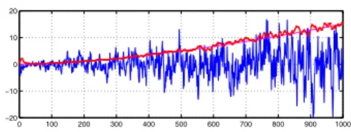
0 100 200 300 400 500 600 700 800 900 1000 Ŧ20 Ŧ10 0 10 20

Fig. 3. Ec model on fractional B-spline. A snapshot of the pro-cess with H = 0.8 and α = 0.3, superimposed with its standard deviation (dots on dashed line, estimated on 1024 realizations; ).

useful to test their scale invariance, because the wavelet coef-ficients at one scale are nonstationary. That is why we have preferred here to show scale invariance directly from the co-variances.

6. REFERENCES

[1] B. Mandelbrot and J. W. Van Ness, “Fractional Brownian mo-tions, fractional Brownian noises and applicamo-tions,” SIAM

re-view, vol. 10, pp. 422–437, 1968.

[2] H. L. Gray and N. F. Zhang, “On a class of nonstationary processes,” Journal of Time Series Analysis, vol. 9, no. 2, pp. 133–154, 1988.

[3] G. Wornell, Signal processing with fractals: a wavelet-based

approach, Prentice Hall, 1996.

[4] B. Yazici and R. L. Kashyap, “A class of second-order station-ary self-similar processes for 1/f phenomena,” IEEE Trans.

on Signal Proc., vol. 45, no. 2, pp. 396–410, 1997.

[5] E. Noret and M. Guglielmi, “Mod´elisation et synth`ese d’une classe de signaux auto-similaires et `a m´emoire longue,” in

Proc. Conf. Delft (NL) : Fractals in Engineering. 1999, pp. 301–315, INRIA.

[6] P. Flandrin, P. Borgnat, and P.-O. Amblard, “From station-arity to self-similstation-arity, and back : Variations on the Lamperti transformation,” in Processes with Long-Range Correlations:

Theory and Applications, G. Raganjaran and M. Ding, Eds. June 2003, vol. 621 of Lectures Notes in Physics, pp. 88–117, Springer-Verlag.

[7] A. Vid´acs and J. Virtamo, “ML estimation of the parameters of fBm traffic with geometrical sampling,” in IFIP TC6, Int. Conf.

on Broadband communications ’99. Nov. 1999, Hong-Kong. [8] V. Girardin and M. Rachdi, “Spectral density estimation from

random sampling for m-stationary processes,” Comput. &

Math. Appli., vol. 46, no. 7, pp. 1009–1021, 2003.

[9] L. Jackson, Digital filters and signal processing, Kluwer, 1989. [10] M. Unser, “Sampling – 50 years after Shannon,” Proce. of the

IEEE, vol. 88, no. 4, pp. 569–587, Apr. 2000.

[11] M. Unser and T Blu, “Fractional splines and wavelets,” SIAM

Review, vol. 42, no. 1, pp. 43–67, 2000.

[12] S. Lee, W. Zhao, R. Narasimha, and R. Rao, “Discrete-time models for statistically self-similar signals,” IEEE Trans. on

Signal Proce., vol. 51, no. 5, pp. 1221–1230, May 2003. [13] P. Borgnat, P. Flandrin, and P.-O. Amblard, “Stochastic

dis-crete scale invariance,” Signal Processing Lett., vol. 9, no. 6, pp. 181–184, June 2002.