HAL Id: tel-02986378
https://hal.archives-ouvertes.fr/tel-02986378
Submitted on 2 Nov 2020HAL is a multi-disciplinary open access archive for the deposit and dissemination of sci-entific research documents, whether they are pub-lished or not. The documents may come from teaching and research institutions in France or abroad, or from public or private research centers.
L’archive ouverte pluridisciplinaire HAL, est destinée au dépôt et à la diffusion de documents scientifiques de niveau recherche, publiés ou non, émanant des établissements d’enseignement et de recherche français ou étrangers, des laboratoires publics ou privés.
to reduce GHG emissions from fires. A case study in
tropical peatlands in Ogan Komering Ilir, Indonesia
María José Rodriguez Vasquez
To cite this version:
María José Rodriguez Vasquez. Evaluation of different peatland management scenarios to reduce GHG emissions from fires. A case study in tropical peatlands in Ogan Komering Ilir, Indonesia. Environmental and Society. AgroParisTech, 2020. English. �tel-02986378�
N : 2020AGPT0002
présentée et soutenue publiquement par
María José RODRIGUEZ VASQUEZ
le 21 juillet 2020Evaluation of different peatland management scenarios to
reduce GHG emissions from fires.
A case study in tropical peatlands in Ogan Komering Ilir,
Indonesia
Doctorat AgroParisTech
T H È S E
pour obtenir le grade de docteur délivré par
L’Institut des Sciences et Industries
du Vivant et de l’Environnement
(AgroParisTech)
Spécialité : Biologie et écologie des forêts et des agrosystèmes
Jury
Mme Marie-Noëlle PONS, Directrice de recherche, CNRS Président & Examinatrice M. Guillaume BOISSONNET, Ingénieur - chercheur (HDR), CEA Rapporteur & Examinateur M. Sébastien GADAL, Professeur, Aix-Marseille Université Rapporteur & Examinateur Mme Cécile BESSOU, Chercheuse, CIRAD Examinatrice
M. Mathieu FORTIN, Ingénieur - chercheur (HDR), Canadian Forest Service Directeur de thèse M. Jean-Marc RODA, Chercheur, CIRAD - Directeur de recherche, UPM Co-directeur de thèse M. Anthony BENOIST, Chercheur, CIRAD Invité/Co-encadrant de thèse
Directeur de thèse : Mathieu FORTIN et Jean-Marc RODA Co-encadrement de la thèse : Anthony BENOIST
This thesis is financed by the University of Costa Rica (UCR), with financial and technical support from the French Agricultural Research Centre for International Development (CIRAD) and the University Putra Malaysia (UPM).
Acknowledgements
Acknowledgements
In September 2015, I left my country to undertake a new experience on the other side of the world. The goal was to do a master's and doctoral program, to learn a new language and to get to know a new culture. Today, in 2020, I return to my country with the objective fulfilled, and with many more experiences that surprised me along the way. I want to thank all the people who made me feel at home and who made this experience much more enriching and welcoming for me.
I would first like to thank my three main thesis advisors: Dr. Mathieu Fortin for his advice, for his support and for his patience throughout the thesis, for his sense of responsibility and consideration throughout the thesis despite the distance, and for his hospitality during my stay in Nancy; Dr. Jean-Marc Roda for recruiting me and showing his trust in me by making me part of his team, for giving me a broad perspective of the different topics we discussed, and for his hospitality in Malaysia; and Dr. Anthony Benoist for all his support and patience from the beginning to the end of my thesis, for helping me not to lose the main thread when I started to go astray, for his sympathy and for his hospitality in Montpellier. I thank the three of them for everything they taught me, technically and professionally, and for providing me with an excellent example of professional quality that I took back to Costa Rica to put into practice.
I would also like to thank the University of Costa Rica for funding this thesis and the staff in charge of students abroad for their consideration, and Dr. Ricardo Radulovich for his support and for showing me a broad perspective of my topic of interest to start my thesis.
I would like to express my gratitude to all the BioWooEB doctoral students and to my friends in general, to mention only the closest - Adrien, Allya, Gwendal, Luke, Florine, Migue, Huyn, Seb, Val, Luis - and many more that I cannot acknowledge here but who are no less important, for making my stay in Montpellier more enjoyable, for all the discussions, beers, pastis and walks we shared, and the whole BioWooEB unit in general. I would particularly like to thank LoÏc for his support and optimism in the final stages of the thesis.
I am also grateful to the "Dream team" of the Universiti Putra Malasya for their sympathy, hospitality and technical support in the field, especially Candice for her enthusiasm, good company and for showing me the best restaurants in Malaysia. Terima kasih.
Finally, I would like to thank my mom, dad and sister wholeheartedly, who were unconditionally there from the beginning to the end of this experience, accompanying me from a distance and giving me all their support. I am also deeply indebted to my family, in general, and to my best friend Rebe, who were always present when I needed them.
Thank you very much! María
Extended abstract
Three percent of total land mass is covered by peatlands, predominately in boreal zones (83 %), followed by tropical (12.7 %) and temperate (4 %) zones. Of this, the 12.7% of tropical peatlands in South America constitute the largest area (46 %), followed by Asia (36 %) and Africa (18 %). This type of ecosystem in the tropics plays an important role as a carbon pool, storing approximately 350,000 Tg of carbon. In Southeast Asia, the carbon stored in peatlands is estimated at around 68,500 Tg.
Over the last decades, changes in land use and land management practices in forestry and agricultural plantations have led to a significant amount of carbon loss. On peatlands, land preparation for agricultural or pulpwood plantations requires drainage and fires in order to create proper conditions for more intensive agricultural uses. Cleaning fields with fire is a traditional practice used by migrant farmers, private companies and government agencies. During a peatland fire, the aboveground biomass is combusted, as is a layer of peat soil. Peat soil fires are usually characterized by smoldering combustion. Smoldering combustion implies a slow and persistent process, largely responsible for expanding fires. This type of combustion can continue to expand underground, vertically until it reaches the water table, or horizontally as residual smoldering combustion (RSC) after surface fires. Recent fires in Indonesian peatlands released a large amount of greenhouse gases (GHGs) into the atmosphere. These fires also affected the economy and the human health of the inhabitants of Indonesia and its neighboring countries. Among the most relevant episodes are the ones that occurred in 1997-98, 2006 and 2015, during the El Niño-Southern Oscillation event.
To address this problem of peat fires that affect Indonesia and its neighboring countries, the government adopted policies, regulations, technical innovations, developments in fire monitoring and incentives to improve land management. After the fire episode of 2015, the fire alerts decreased. However, despite these measures, the fires continue in the region. The main reasons why fires continue include the failure to apply policies and regulations, the lack of incentives, the lack of technical knowledge and information about not burning clear land, and cultural aspects (e.g., the traditional use of fire).
In this thesis, we evaluated different mitigation scenarios as an option to reduce fires, converting aboveground biomass into bioenergy or other bio-products instead of burning it and, at the same time, creating incentives for the local population.
The main three objectives of the thesis are: (i) to determine the greenhouse gas emissions associated with the current fires in agricultural and forest areas on tropical peatlands; (ii) to quantify avoided emissions of peat soil combustion and to evaluate the sustainability of alternative scenarios based on the use of aboveground biomass for bioenergy production and other by-products; and (iii) to identify socio-economic and political determinants to promote the use of biomass on peatlands for bioenergy production. These objectives are developed in four chapters. In Chapter 1, we propose a general equation to estimate GHG emissions from fires on peatlands. We used Monte Carlo simulation, meta-analyses, and an analytical expression of variance. The contribution of each parameter to the variance of the estimated GHG emissions was also evaluated. GHG emissions of a single fire episode were estimated at 842 Mg ha-1 CO
2-eq, with a
standard deviation of 466 Mg ha-1 CO
2-eq. Our estimated GHG emissions were close to the amount
estimated from the default values provided by the IPCC. The main parameters contributing to variance were: the depth of burn: 94.2 %; followed by bulk density: 5.5 %; and emission factors:
0.3 %. When the depth of burn was assessed by remote sensing, the main contributor to variance became the fire-damaged area, followed by the depth of burn. The contribution of each parameter to variance, as estimated in this study, made it possible to prioritize the effort in uncertainty reduction. Combining Monte Carlo simulation and an analytical expression of variance could be a promising way of obtaining more reliable confidence intervals.
Chapter 2 contains three parts. Part I presents the study area, Ogan Komering Ilir (OKI) and the
context in which the assessments were carried out. I focused on the three major land uses on peat soils in OKI, which are also considered for their potential biomass for valorization: (i) degraded peatlands; (ii) oil palm plantations; and (iii) pulpwood plantations. Pulpwood plantations cover most of the plantation area.
In Part II, an analysis of the fire occurrence in OKI was carried out to estimate the GHG emissions from peat combustion for the three aforementioned land use types at the regional level for the period 2002-2018. The results showed that 70%, 45% and 76% of the pixels in degraded peatlands, oil palm plantations and pulpwood plantations, respectively, were affected by fires during the period 2002-2018. The total GHG emissions from peat soil combustion estimated for this period was 76x106 Mg CO
2-eq for degraded peatlands, 36x106 Mg CO2-eq for oil palm plantations and
321x106 Mg CO
2-eq for pulpwood plantations. Pulpwood plantations were the greatest contributor
of GHG emissions in OKI due to the large area of the plantations in the study area, the highest percentage of pixels with fire occurrence and the largest fire-damaged area affected by pixels among the three land uses.
In Part III, a distance assessment for biomass transportation to five potential industry locations was performed. The objective was to estimate the influence of the distance of biomass transportation on the total GHG emissions calculated in Chapter 3, and the influence of the distance on transportation costs in Chapter 4. The distance assessment performed is based on the geodata of roads and waterways provided by recent studies in the same area. We found that waterways provided the widest access to the study zone. The average distance from any point to the nearest waterway was 49 km (min=0, max=233), whereas the average distance to the nearest road was 122 km (min=0, max=347). The average distance to the nearest road or waterway in the study area was 23 km (min=0, max=133). We noted that Palembang, Pedemaran and Secukai have access to both types of networks, which allows a greater access to biomass resources throughout the year. APP and Sungai Lumpur locations were limited to waterways. This assessment made it possible to identify the most distant areas, which were then evaluated in detail in the next chapters using different indicators.
In Chapter 3, several mitigation scenarios of land management are analyzed to compare their global contribution to climate change in terms of CO2-eqwith business as usual (BAU) scenarios.
For this purpose, three types of biomass corresponding to the three land uses analyzed in this study were considered for bioethanol production, combined heat and power generation and panel manufacturing. The five scenarios evaluated are: (1) BAU with fire occurrence; (2) BAU without fire occurrence; (3) prospective biomass valorization in drained conditions, (4) prospective biomass valorization in non-drained conditions; and (5) peatland restoration. The impact of each scenario for the three land uses considered in this study was estimated on the basis of life cycle assessment methodology. GHG emissions estimated for BAU with a fire occurrence scenario in degraded peatland, oil palm plantations and pulpwood plantations were 70.60±30, 139.40±31 and 159± Mg CO2-eq ha-1 yr-1, respectively. For BAU without a fire occurrence scenario in degraded peatland, oil
108.3±15 Mg CO2-eq ha-1 yr-1, respectively. Regarding the restoration scenario, the estimated GHG
emissions were the same for the three land uses: -0.9 Mg CO2-eq ha-1 yr-1.
Regarding scenarios of biomass valorization with a functional unit of 1 hectare during a year (1hayr), in the case of degraded peatland, valorizing the biomass reduces the GHG emissions by about 74 % in drained conditions and 99 % in non-drained conditions, compared with BAU with a fire occurrence scenario. For oil palm plantations, valorizing the biomass reduces the GHG emissions by about 60 % in drained conditions compared with BAU with a fire occurrence scenario. In pulpwood plantations, the reduction for valorizing the biomass is about 40 % of GHG emissions in drained conditions compared with BAU with a fire occurrence scenario.
The scenarios in non-drained conditions significantly reduce the GHG emissions in comparison to BAU because they reduce the flux gases from peat oxidation and allow carbon sequestration in peat soil. However, scenarios in non-drained conditions are only considered for degraded peatland because waterlogging conditions are not adequate for oil palm and pulpwood cropping systems. The scenarios of biomass valorization in non-drained conditions are an example of paludiculture systems, where the plantations could be managed in waterlogging.
Regarding the carbon balance at the regional level, we predicted a reduction of the impact by 2-10 % of the GHG emissions for implementing biomass valorization. Biomass valorization is an option to decrease the haze from fires that have an impact on climate change as well as causing other kinds of problems such as health issues caused by fine particular matter (PM2.5) or economic
losses associated with the haze for land management with fires.
In Chapter 4, we assessed the socio-economic factors for implementing mitigation scenarios in the three main land uses studied in this work for the OKI district. We focused on the factors that are critical for fire mitigation through biomass valorization. We compared different strategies toward potential reduction of GHG emissions and costs for the three main land uses. We computed the areas where the biomass market is feasible according to each potential factory location. We found that valorizing the biomass in the areas where the biomass market is feasible reduced GHG emissions by 4-6 %, compared with BAU in OKI. The rest of the biomass contained in the areas where the biomass market is not feasible cannot be valorized by the industry. Boosting the biomass market in the feasible areas identified in this study can reduce the GHG emissions without governmental investments in these areas. This makes it possible to prioritize government investments aimed at reducing GHG emissions from peatlands in areas where the biomass market is not feasible. In addition, the land management scenarios evaluated here can provide a new income for local populations that could take advantage of the biomass residues that are currently combusted on peatland.
Table of contents
Acknowledgements ... iii
Abstract ... vi
Table of contents ... x
Introduction ... 13
Estimating greenhouse gas emissions from peat combustion in wildfires on Indonesian peatlands, and their uncertainty ... 23
General assessments ... 47
Life cycle greenhouse gas emissions of biomass valorization in OKI ... 67
Socio-economic assessment of emission mitigation scenarios in OKI ... 95
Synthesis ... 113
References ... 119
1. Peatlands in the world
Three percent of total land mass is covered by peatlands, predominately in boreal (83 %) followed by tropical (12.7 %) and temperate (4 %) zones. The main areas in boreal and temperate zones are in Canada, the British Isles, Fennoscandia, the Baltic States and Russia (Leifeld & Menichetti, 2018). In tropical zones, South America constitutes the largest area of tropical peatlands (46 %), followed by Asia (36 %) and Africa (18 %) (Gumbricht et al., 2017).
Peatlands are included in the wetlands classification defined by the Ramsar Convention on Wetlands. Ramsar (2016) defines wetlands as “areas of marsh, fen, peatland or water, whether natural or artificial, permanent or temporary, with water that is static or flowing, fresh, brackish or salt, including areas of marine water the depth of which at low tide does not exceed six meters”. Peatland refers to the area where peat accumulates at the surface with or without vegetation (Biancalani & Avagyan, 2014; Joosten & Clarke, 2002).
According to the international soil classification (IUSS Working Group WRB, 2015), peat soils belong to the “histosols” or “organic soil” classes. Soils are qualified as such when dead organic matter accounts for at least 30 % of their dry mass (FAO, 1998), in addition to high water saturation levels and low levels of oxygen (Biancalani & Avagyan, 2014; FAO, 1998). Peat soils have high carbon contents, 55 % on average in the tropical zones (Hu et al., 2018; Konecny et al., 2016; Limin et al., 2004; Page et al., 2011) and 47% in the boreal zones (Cancellieri et al., 2012; Hatch et al., 2015; Hu et al., 2018).
The main ecosystem services provided by peatlands are carbon storage, climate regulation and water regulation (Kimmel & Mander, 2010). Peat areas are also used for installing agriculture, horticulture and forestry plantations.
2. Peat formation and carbon dynamics
Peat formation is a very slow process resulting from the fact that net primary production is higher than the decomposition rate (Chimner & Ewel, 2005; Joosten et al., 2012). The biomass can come from grasses, shrubs, crops or any type of vegetation that grows in these areas. Peat formation also requires waterlogging, which leads to the anaerobic conditions responsible for the slow decomposition (Page et al., 2004; Ritzema & Wösten, 2006).
The peat system is composed of two layers. The upper layer, known as the acrotelm, corresponds to the 10-75 cm aerobic layer with high hydraulic conductivity (Clymo, 1984; Ingram, 1978; Lindsay et al., 2010). The second layer, underneath, is older and usually several meters deep. It is known as the catotelm and usually presents anaerobic conditions and low hydraulic conductivity (Clymo, 1984; Ingram, 1978). The acrotelm is composed of living plant material, bacteria, microorganisms and dead organic matter. The catotelm is an inert carbon accumulation layer, fed by the acrotelm layer, where the biomass decomposition rate is lower than in the upper layer (Lindsay et al., 2010).
Plant parts with high lignin content accumulate in the acrotelm and contribute to peat formation (Parish et al., 2008). Leaves are almost always decomposed, even in anaerobic conditions (Gomez & Yule, 2009), and the roots and thick stems are the greatest contributors to peat formation in the tropics (Brady, 2004; Chimner & Ewel, 2005; Hoyos-Santillan et al., 2015). Organic matter accumulation in the acrotelm layer is a key condition for peat formation and accumulation in the catotelm layer. However, in waterlogging conditions, even without any input of organic matter, the peat layer is preserved from decomposition. In aerobic conditions, for example, when the water table lowers due to drainage or climatic phenomena such as the El Niño-Southern Oscillation (ENSO) event,
3. Management issue in Southeast Asian peatlands
the carbon stored in peat soil is released into the atmosphere by peat oxidation. Under conditions of water saturation and low oxygen, carbon is mostly emitted as methane (CH4) (Bridgham et al., 2013;
Eggleston et al., 2006). This process is known as heterotrophic respiration and only involves the microbial decomposition of soil organic matter (Matysek et al., 2018).
This type of ecosystem in the tropics is a major carbon pool (Leng et al., 2019), storing approximately 350,000 Tg of C (Gumbricht et al., 2017). In Southeast Asia, the carbon stored in peatlands is estimated at around 68,500 Tg of C (Page et al., 2011).
3. Management issue in Southeast Asian peatlands
Over the last decades, the forest cover in Southeast Asian peatlands has decreased by around 42% due to land use change (Miettinen & Liew, 2010). These land use changes release a significant amount of carbon into the atmosphere due to peat oxidation. The peat subsidence in oil palm (Elaeis sp.) and acacia (Acacia mangium) plantations is estimated to be approximately -4 and -5 cm yr-1, which is
explained by the water table level (Evans et al., 2019; Khasanah & van Noordwijk, 2019). One of the reasons for these land use changes is the increasing demand for palm oil and pulpwood that has led to an increase in planting areas (Fig. 1). Today, in South Sumatra, approximately 60 % of the land cover on peatlands consists of oil palm and pulpwood plantations, with a majority of industrial plantations (Miettinen et al., 2016).
Figure 1. Expansion of industrial plantations in the peatlands of Sumatra. Adapted from Miettinen et al. (2016).
On peatlands, land preparation for agriculture or forestry plantations requires drainage and fire in order to create proper conditions for more intensive agricultural uses (Farmer et al., 2011).
Cleaning fields with fire is a traditional practice used by migrant farmers, private companies and government agencies (Page et al., 2002). Land clearing is the major cause of fire but fires can also result from land tenure, resource extraction, hunting or by accident (Applegate et al., 2001). Peat soil fires are usually characterized by smoldering combustion. Smoldering combustion implies a slow and persistent process, largely responsible for expanding fires (Huang & Rein, 2018). This type of combustion can keep expanding underground, vertically until it reaches the water table, or horizontally as residual smoldering combustion (RSC) after surface fires (Akagi et al., 2011; Bertschi
et al., 2003; Usup et al., 2004). Smoldering combustion can spread for days or months, and if not stopped it can even reignite the fire in the next dry season (Huang & Rein, 2018). Although the moisture content slows down its propagation, the fire can continue drying peat soil layers and spreading through them below the ground surface, even at a 200% moisture content (Prat et al., 2013). Due to the fire behavior and high carbon content of peat soil, around 70% of total carbon emissions come from the burning of peat soil. The remaining 30% come from aboveground biomass burning (Page et al., 2002; Van der Werf et al., 2010).
Recent fire episodes in Indonesian peatlands released large amounts of GreenHouse Gases (GHGs) into the atmosphere. These fires also affect the economy and human health of the inhabitants of Indonesia and its neighboring countries. Among the most relevant are the fire episodes that occurred in 1997-98, 2006 and 2015, during ENSO events (Fig. 2) (Huijnen et al., 2016). To illustrate the magnitude of these fire episodes influenced by ENSO events, in 1997-98, fires affected an area of between 1 and 7 million hectares, including large areas of peat bogs in Sumatra, Indonesia, representing between 13% and 40% of global anthropogenic carbon emissions from fossil fuel (Page et al., 2002).
The haze produced during fires and RSC causes air pollution at levels harmful to humans (Hansson & Dargusch, 2017). In addition to carbon, the smoke contains sulfur, benzene, methylene chloride, nitrogen oxides, particulates, volatile organic compounds and other components, prevailing particulate matter PM2.5, as well as PM10 and PM1 (Blake et al., 2009). These compounds are highly irritating and some are carcinogenic. It is estimated that they caused 100,000 premature deaths in Indonesia, Malaysia, and Singapore during 2015 and cost the Indonesian economy some US$16.1 billion (World Resources Institute, 2016; Hansson & Dargusch, 2017).
4. Peatland policies in Indonesia
After the 2015 fire episode, Indonesian President Joko Widodo declared a national state of emergency for fires. The same year, Indonesia made a commitment to the United Nations Framework Convention on Climate Change (UNFCCC) to reduce its GHG emissions by 29% by 2030 and ratified the target in the Paris Agreement in November 2016 (Wijaya et al., 2017). The five priority sectors considered by the government for the reduction of GHG emissions are: forestry and peatlands, agriculture, energy and transportation, industry and waste. This PhD mainly focuses on peatland fires in Indonesia, involving priority sectors such as agriculture and energy and their relationships with peatlands.
In an attempt to address this issue of Indonesian peatland fires, which affects the entire region, the government adopted the Fire Management Interventions (FMI) program that includes policies, regulations, technical innovations and developments in fire monitoring, as well as incentives for improved land management (Carmenta et al., 2017). FMI are supported by the intergovernmental Association of Southeast Asian Nations (ASEAN), through the Agreement on Transboundary Haze Pollution, Peatland Management Strategy, Sustainable Use of Peatland and Haze Mitigation programs, among others (ASEAN, 2019; Sunchindah, 2015). In addition to these programs, in 1999, the ASEAN Ministers of Environment adopted the “Zero-burning” policy to be applied to agricultural and forestry plantations with the aim of avoiding transboundary haze pollution (Secretariat, 2003). Several techniques of “Zero burning” were implemented, mostly in oil palm plantations.
Regarding the Indonesian peatland policies and regulations, the four main peatland government regulations are: (1) control of natural damage and/or pollution related to land and forest fires; (2) guidance for the utilization of peatland for oil palm cultivation; (3) improvement of governance of
4. Peatland policies in Indonesia
natural primary forest and peatland; and (4) protection and management of peatland ecosystems (Uda et al., 2018).
In 2016, the Indonesian president created the Peat Restoration Agency (Badan Restorasi Gambut; BRG) with the objective of restoring 2.1 million hectares of peatlands by 2020, with a priority on those burned in the fire episode of 2015 (CIFOR, 2016). In the same year, the president issued Presidential Decree No. 9/2016 on the acceleration of the implementation of One Map. One Map is a tool for identifying overlapping licenses of forest concessions, industrial forest plantations and mining areas with protected natural forests in order to avoid land tenure conflicts, especially due to the use of fire as a means of land clearing (Shahab, 2016).
Municipal governments have been working with non-governmental organizations (NGOs) and academic researchers to comply with these regulations. Mainly, they attempt to implement zero-burning techniques, peatland restoration, water table monitoring and responsible oil palm plantation such as the Roundtable on Sustainable Palm Oil (RSPO), and to plan possible paludiculture programs (e.g., Indonesia Wetlands International, WWF Central Kalimantan, Walhi, WARSI-Jambi, FFA, etc.) (Uda et al., 2018). For example, the NGO “Free Fires Alliance” (FFA) has been working since 2016 with incentive programs that have proven themselves to be successful, e.g., “No burn village rewards” that are awarded at the end of the dry season: IDR 100 mill for a burnt area of less than 1 ha, and IDR1 50
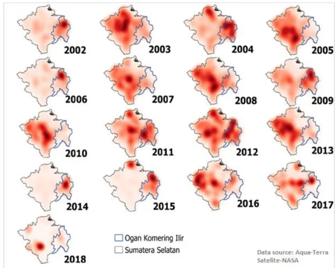
mill for a burnt area of less than 10 ha (FFA, 2016). After the fire episode of 2015, the alerts decreased, in part thanks to the policies, regulations and efforts of the NGOs and the communities involved. However, the fire alerts continue in the region and underwent a major increase in 2019, aggravated by a very dry season (Fig. 2).
Figure 2. Number of fire alerts for the period from June 2002 to December 2019. Data source from Aqua-Terra satellites, NASA. (A) Fire alerts per year for the period from June 2002 to February 2020, and the mean of fire alerts for the same period. (B) Mean of fire alerts per year.
The main reasons why fires continue were a failure to apply policies and regulations, the lack of technical knowledge and information about not burning clear land, cultural aspects, e.g., traditional use of fire, and lack of incentives (Carmenta et al., 2017; Tacconi, 2016; Uda et al., 2018).
5. Current state of renewable energy in Indonesia
Providing electricity in an archipelago of 17,000 islands is technically challenging. Nevertheless, in 2014, Indonesia had access to electricity over 84 % of its territory (Asian Development Bank, 2016). This proportion increased to 95.35 % in 2017 (PwC Indonesia, 2018). The area with the least access to electricity corresponds to the southeast part of Indonesia. In 2017, the power capacity was 60.7 GW, 57.2 % of which comes from coal, 24.8 % from gas, 5.8 % from oil and 12.5 % from renewable energy. Among renewable energy sources, hydropower and geothermal are the main renewable energy sources, contributing 7.3 % and 5 %, respectively, to the total renewable energy. The rest (0.2 %) comes from bioenergy and solar. However, the 2018 Price Waterhouse and Coopers (PwC) Indonesia report estimated a bioenergy potential of 32.6 GW that can be harnessed.
Regarding energy policies, the “State-owned electricity company” (PLN) plans to increase the renewable energy share to 23 % by 2025 and 31 % by 2050. This increase would involve raising the current energy shares by 10 % for bioenergy, 7 % for geothermal, 3 % for hydropower and 3 % for other new and renewable energies. In order to encourage the public and private sectors to implement new projects on renewable energy, the government has established fiscal incentives such as a reduction in taxable income, an extended tax loss, accelerated depreciation and amortization rates, and exemption for imports via import parity prices involved in renewable energy (PwC Indonesia, 2018).
6. Research positioning and objectives
Economic development in poor or developing countries denotes, in the majority of cases, the exploitation of natural resources to the point of threatening environmental sustainability (Purvis et al., 2019). This disproportionate economic development has led to social and environmental issues. This has engendered concepts such as ‘eco-development’ (CIDA, 1979) or ‘sustainability development’ (WCED, 1987), with the objective to find a fair “balance between the economic and social systems and ecological conditions”. This is also known as the “three pillars” or the “triangle of sustainability” (Keiner, 2005). In this thesis, I evaluated the business as usual peatland management in Ogan Komering Ilir (OKI) and then compared it with other scenarios that propose to continue economic activities on peatlands but that implement practices that would make it possible to find an environmental balance.
The French Agricultural Research Centre for International Development (CIRAD) contributed to the creation of the “Center of Excellence” (COE) project, together with Airbus Malaysia, the Aerospace Malaysia Innovation Centre (AMIC), the UPM (Universiti Putra Malaysia) and the Malaysian Industry-Government Group for High Technology (MIGHT). The objective of the COE is to carry out a bio-jetfuel project based on the use of agricultural residues to reduce fossil fuel consumption. CIRAD has been working on biomass recovery in Malaysia and Indonesia for bio-jetfuel production, as well as transportation and cost scenarios concerning biomass.
Within the framework of the COE and taking the issue of fire haze in Indonesia into account, biomass valorization has been suggested as an option to reduce fire occurrences and to convert aboveground biomass into bioenergy or other bio-products instead of burning it.
7. Thesis overview
In accordance with this and focusing on the reduction of fires, we defined the following objectives of the thesis:
1. Determine the greenhouse gas emissions associated with the current fires in agricultural and forest areas on tropical peatlands.
2. Quantify avoided emissions of peat soil combustion and evaluate the feasibility and sustainability of alternative scenarios based on the use of aboveground biomass for bioenergy production and other bio-products.
3. Identify socio-economic and political determinants to promote the implementation of different mitigation scenarios in OKI.
7. Thesis overview
My thesis project is developed in four main chapters (Fig. 3):
Chapter 1: Greenhouse gas emissions from peat soil combustion in wildfires on Indonesian peatlands Chapter 2: General assessments
Chapter 3: Life cycle greenhouse gas emissions of different land use management scenarios in OKI Chapter 4: Socio-economic assessment of emission mitigation scenarios in OKI
In Chapter 1, I focused on the main problem that motivated this thesis: the fires in tropical peatlands. This chapter provides a perspective of the current situation in Southeast Asian peatlands and an estimate of the GHG emissions from peat soil combusted in wildfires in terms of CO2-eq ha-1.
Given that fires are a local problem but have an impact at a larger scale, i.e., transboundary haze in Southeast Asia and a direct impact on climate change, we analyzed, from Chapter 2 onwards, different land management scenarios through a case study at Ogan Komering Ilir (OKI). Chapter 2 provides the basic information and the parameters used throughout the thesis to develop the different scenarios of land management on peatlands in OKI. Specifically, Part I presents the study area, and Part II provides an estimate of the GHG emissions resulting from peat combustion related to fire activity for the whole study area. This estimate was a prerequisite for Chapter 3 in which it stands for a “Business as usual” scenario in comparisons with different mitigation scenarios. Finally, in Part III, an assessment of the distance related to biomass transportation was performed, assuming different factory locations. This assessment was also used to evaluate the impact of biomass transportation in terms of GHG emissions in Chapter 3 and the transportation cost of biomass to the factories in Chapter 4.
In keeping with this, in Chapter 3, I estimated the GHG emissions of the business as usual and mitigation scenarios in OKI. The mitigation scenarios are based on different land use management scenarios where potential biomass valorization is evaluated as an alternative to cleaning peatlands with fires. The impact of each scenario was estimated in terms of CO2 equivalent.
Finally, in Chapter 4, I assessed the socio-economic factors for implementing mitigation scenarios in the three main land uses investigated in this study for the OKI district. Different strategies for the potential reduction of GHG emissions and costs were compared for the three main land uses. The main parameters were fire occurrence, potential biomass and transportation costs.
Estimating greenhouse gas emissions from peat combustion in wildfires on
Indonesian peatlands, and their uncertainty
Scope of Chapter 1.
In Chapter 1, we focused in the central issue that motivated this thesis: wildfires in peatlands. This chapter offers a perspective of the current situation in Southeast Asian peatlands and provides an estimate of the impact on climate change of the peat soil combusted in wildfires in terms of CO2-eq.
The uncertainty and the contribution of each parameter involved in the estimation are provided. This estimate is used in the following chapters to establish the business as usual scenarios and to then compare them with the other land management scenarios proposed.
This chapter is based on:
M. J. Rodríguez Vásquez, A. Benoist, J.-M. Roda, M. Fortin (submitted). Estimating greenhouse gas emissions from peat combustion in wildfires on Indonesian peatlands, and their uncertainty. Biogeochemical Cycles.
1. Introduction
Since 1982, the peatlands of Southeast Asia have suffered from depletion due to economic pressure and the demand for natural resources, often caused by fires on forest and agricultural land. The rate of land use change in Indonesia has been increasing due to pulpwood plantations and agriculture, mainly for oil palm plantations (Evers et al., 2016; Miettinen et al., 2016; Padfield et al., 2019). On peatlands, land preparation for agriculture or pulpwood plantations requires drainage in order to create proper conditions for more intensive agricultural uses (Farmer et al., 2011). When the peatland is drained, the carbon stored in peat soil is released into the atmosphere by peat oxidation under aerobic conditions. Besides the emissions from drainage, another way for the carbon of peatlands to enter the atmosphere is through fires. Around 70 % of total carbon emissions following peatland fires come from the burning of peat soil, while the remaining 30 % come from aboveground biomass burning (Page et al., 2002; Van der Werf et al., 2010).
Fires in Indonesian peatlands can have an important impact on climate change because of the large amount of GreenHouse Gases (GHGs) they released in the atmosphere. These fires also affect the economy and human health of the inhabitants of Indonesia and neighboring countries. Important fire episodes in Indonesian peatlands occurred in 1997-98 and 2015, both during the ENSO event (Huijnen et al., 2016). During the episode of 1997-98, fires affected an area between 1 and 7 million hectares, including large areas of peat bogs in Sumatra, Indonesia, representing between 13 % and 40 % of global anthropogenic carbon emissions estimated for 1998 (Page et al., 2002).
The impact of peatland fires in terms of carbon emissions has been addressed in many studies (Ballhorn et al., 2009; Konecny et al., 2016; Page et al., 2002; Van der Werf et al., 2010). While estimated carbon emissions vary greatly across the different fire episodes, there is a constant in these studies: the estimates are all subject to large uncertainties. There are actually many parameters involved in estimating carbon emissions and the uncertainty surrounding each one of them is not well known. In many studies, the authors had to rely on the best guess when it came to estimating the uncertainty related to certain parameters. Moreover, when those studies provided uncertainty in the estimated carbon emissions, it remained unclear as to which parameter induced the greatest share of uncertainty.
The IPCC guidelines (Hiraishi et al., 2014) provide a general equation to estimate the impact of peatland fires in terms of GHG emissions, as well as default values for the mass of fuel available for combustion. However, the appraisal of each parameter is rarely provided. The mean and the variance of the parameters change, even within the same geographical area, with the values sometimes being very different. This variability is conditioned by factors such as the fire episode, land use and water table level (Heil et al., 2007).
In this study, we conducted a literature review on GHG emissions from peatland wildfires in Southeast Asia, and a meta-analysis on the parameters used to estimate their impact on climate change in terms of CO2 equivalent. Using CO2 equivalent made it possible to consider the combined
global warming potential of different GHG in the atmosphere and to compare the relative contributions of GHG (Myhre et al., 2013). The objectives were to 1) define a general equation to estimate GHG emissions, 2) define default values for its parameters based on what is currently known of the different fire episodes and 3) evaluate the individual contributions of those parameters to the uncertainty of estimated GHG emissions.
Two approaches were taken to estimate GHG emissions and evaluate the uncertainty related to that estimate. The first was a “retrospective” approach and the second was a “prospective” approach.
2. Materials and Methods
The retrospective approach assumed that the fire episode has already occurred and that some parameters were already available. The prospective approach consisted of obtaining more accurate default values and providing recommendations for the use of certain parameters when estimating GHG emissions during future fire episodes.
2. Materials and Methods
2.1 Estimating the impact of peatland wildfires on climate change
In the literature, the impact of peatland wildfires on climate change is estimated through two indicators: GHG emissions and carbon loss. The first seeks to quantify GHG emissions and is described in the IPCC guidelines (Hiraishi et al., 2014). It can be expressed as follows:
𝐿𝑓𝑖𝑟𝑒 = 𝐴 × 𝑀𝐵× 𝐶𝑓× 𝐺𝑒𝑓× 10−3 (1-1)
where Lfire is the emission of a particular GHG (Mg), A is the total fire-damaged area (ha), MB is the
mass of fuel available for combustion (Mg ha-1), C
f is a dimensionless combustion factor, and Gef is
the emission factor of that particular GHG (kg Mg-1 of dry matter burnt). Note that the 10-3 factor
ensures proper unit conversion. The total GHG emissions are then estimated by summing the Lfire of
the individual GHGs after their conversion into CO2 equivalent through their respective Global
Warming Potential (GWP).
The second method focuses on carbon losses only (Ballhorn et al., 2009; Boehm et al., 2001; Page et al., 2002). It can be expressed through the following equation:
Closs= A × P × BD × CC × 104 (1-2)
where Closs is emitted carbon (Mg), A is the total fire-damaged area (ha), P is the average depth of
burn (m), BD is the average bulk density of peat soil (Mg m-3) and CC is the average carbon content
of peat soil (Mg of C per Mg of peat soil). Again, the 104 factor ensures proper unit conversion.
Eq. 1-1 and 1-2 have different purposes and therefore different expressions. However, the quantification of GHG emissions in Eq. 1-1 is more appropriate than the quantification of carbon losses in Eq. 1-2 to estimate an impact on climate change, since it takes into account different forms of carbon emissions (CO2, CO, CH4) and other GHG emissions (N2O, NOx).
Apart from these considerations of carbon forms and other GHGs, Eq. 1-1 and 1-2 also differ in the way they estimate the amount of burned peat. According to Eq. 1-1, the amount of GHG is considered as proportional to the product of the mass of fuel (MB) by a combustion factor (Cf). The
mass of fuel is “determined by measuring the depth of burn, along with soil bulk density and carbon content” (Hiraishi et al., 2014). These guidelines also specify that under the Tier 1 approach, “the default combustion factor [Cf] is 1.0, which implies that all fuel is combusted (Yokelson et al., 1997)” (Hiraishi et al., 2014). In Eq. 1-2, the amount of burned peat is proportional to the product of the depth of burn by the bulk density. As a matter of fact, Eq. 1-2 can be considered as an elementary expression of Eq. 1-1 under the Tier 1 approach.
In this study, we standardized Eq. 1-1 and 1-2 in order to obtain a more comprehensive estimate of the impact of peat wildfires on climate change. We then chose to quantify GHG emissions as in Eq. 1-1, and to use the elementary structure of Eq. 1-2 to estimate the amount of burned peat, in order
to be explicit in the parameters used. As for Eq.1-1, we adopted the emission factor Gef, where the carbon content is included. Lastly, we explicitly added the GWP of each gas and the sum of the contributions of all GHGs to express the impact on climate change in terms of CO2 equivalent. The
resulting equation is given below:
Efire = A × P × BD × ∑ (G𝑖 ef,i× GWPi)× 10 (1-3)
where Efire is the amount of GHG emissions (Mg of CO2-eq), A is the total fire-damaged area (ha), P
is the average depth of burn (m), BD is the average bulk density of peat soil (Mg m- 3), G
ef is the
average emission factor for each gas (kg Mg- 1dry matter burnt) and GWP is the global warming
potential for each gas (Mg CO2-eq/Mg of gas). All the estimates of GHG emissions in this study were
obtained using Eq. 1-3.
2.2 Data collection
In order to make Eq. 1-3 useable, its parameters needed to be estimated. We gathered studies related to the depth of burn of recent fire episodes, the bulk density of peat soil and CO2, CO, CH4
and NOx emission factors from the existing literature. Their results were assembled into datasets,
which were then analyzed using a meta-analysis approach. This approach has been widely used in many fields of study (Cooper et al., 2019; Gurevitch et al., 2018) and allows for more accurate parameter estimates. The models behind the different meta-analyses that we carried out are detailed in the Meta-analyses section.
Different studies provided the average depth of burn for some fire episodes, through either remote sensing or post-fire field measurements. We managed to retrieve seven of these (Table 1-1). The majority of the studies were conducted in Central Kalimantan during fire episodes that occurred between 1997 and 2011, with the exception of Simpson et al. (2016), who carried out their study in Sumatra.
Table 1-1. Collected data for the estimation of depth of burn.
Author Sample size episode Fire Number of fires
Fire-damaged
area (ha) Depth of burn (m)
Page et al. (2002) 43 1997 1 729 500 0.51 Ballhorn et al. (2009) 41 2006 1 256 783 0.33 CIMTROP in Ballhorn et al. (2009) 40 2006 1 n/a (ii) 0.30 Simpson et al. (2016) 5305 2015 1 5.2 0.23 Boehm et al. (2001) 100 1997 1 796906 0.40 Konecny et al. (2016) 16016 1997-2011(i) 1-8 100 000 0.17 Limin et al. (2004) 108 2002 1 79 609 0.21
(i)Corresponds to fire episodes in 1997, 2001, 2002, 2004, 2005, 2006, 2009 and 2011 (ii)n/a: not available
2. Materials and Methods
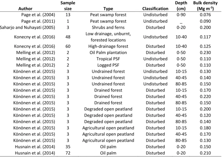
For average bulk density (BD), we found 22 estimates in seven studies from Central Kalimantan, Riau and Jambi in Indonesia, as well as one study from Sarawak, Malaysia (Table 1-2). The area description provided in each publication was used to classify each measurement according to a land cover class. However, the limited information found in the publications and the discrepancies in land cover terminology only allowed to distinguish two classes: disturbed and undisturbed. We classified as disturbed all the study areas that were described as shrubs and ferns, drained, burned, degraded land or agricultural plantations. Likewise, the study areas that were characterized by low drainage, unburnt, forested locations or tropical peat swamp forest were classified as undisturbed, as shown in Table 1-2. For studies that provided information about the density of the soil profile, we used only the data for the first 85 cm, because our emphasis was on the potential depth of burn (see Depth of burn in the Meta-analyses section).
Table 1-2. Collected data for estimation of the bulk density of a tropical peat soil
Author
Sample
size Type Classification
Depth (cm)
Bulk density (Mg m-3) Page et al. (2004) 13 Peat swamp forest Undisturbed 0-90 0.076 Page et al. (2011) 1 Peat swamp forest Undisturbed _ 0.090 Saharjo and Nuhayati (2005) 3 Shrubs and ferns Disturbed 0-20 0.200
Konecny et al. (2016) 48 Low drainage, unburnt,
forested locations Undisturbed 10-40 0.117 Konecny et al. (2016) 60 High-drainage forest Disturbed 10-40 0.125 Melling et al. (2012) 2 Oil Palm plantation Disturbed 0-50 0.230 Melling et al. (2012) 2 Tropical PSF Undisturbed 0-50 0.110
Melling et al. (2012) 2 Logged PSF Disturbed 0-50 0.110
Könönen et al. (2015) 3 Undrained forest Undisturbed 10-15 0.130 Könönen et al. (2015) 3 Undrained forest Undisturbed 40-45 0.140 Könönen et al. (2015) 3 Undrained forest Undisturbed 80-85 0.150 Könönen et al. (2015) 3 Drained forest Disturbed 10-15 0.170 Könönen et al. (2015) 3 Drained forest Disturbed 40-45 0.220 Könönen et al. (2015) 3 Drained forest Disturbed 80-85 0.150 Könönen et al. (2015) 3 Degraded open peatland Disturbed 10-15 0.200 Könönen et al. (2015) 3 Degraded open peatland Disturbed 40-45 0.120 Könönen et al. (2015) 3 Degraded open peatland Disturbed 80-85 0.140 Könönen et al. (2015) 3 Agricultural open peatland Disturbed 10-15 0.180 Könönen et al. (2015) 3 Agricultural open peatland Disturbed 40-45 0.170 Könönen et al. (2015) 3 Agricultural open peatland Disturbed 80-85 0.130
Husnain et al. (2014) 35 Oil palm Disturbed 0-20 0.150
Husnain et al. (2014) 72 Oil palm Disturbed 0-20 0.210
Four gases were considered for emission factors (Gef): carbon dioxide (CO2), carbon monoxide (CO),
methane (CH4) and nitrogen oxides (NOx). We gathered the estimates from four studies (Table 1-3).
Stockwell et al. (2016) estimated an average emission factor for each gas. However, the authors provided their data, so we were able to use their observations instead of their estimates.
Emission factors can actually change depending on dominating combustion conditions, either flaming or smoldering (Akagi et al., 2011). The emissions factors used in this study were measured
under conditions of smoldering combustion, as determined by the modified combustion efficiency (MCE) (Table 1-3). MCE is an index of the degree of combustion, flaming or smoldering combustion, based on the amount of CO2 and CO emitted (Briggs et al., 2016):
𝑀𝐶𝐸 =∆𝐶𝑂∆𝐶𝑂2
2+∆𝐶𝑂 (1-4)
where ΔCO2 and ΔCO are the carbon concentrations expressed by the emission factors of CO2 and
CO, respectively. MCE calculation yields a value between 0 and 1. O2 is rapidly consumed in flaming
combustion, producing oxidized gases such as CO2, H2O, NOx and SO2. On the other hand, in
smoldering combustion, pyrolysis and gasification mechanisms occur, producing CO, CH4,
non-methane organic compounds and primary organic aerosols (Akagi et al., 2011; Stockwell et al., 2016). Nevertheless, flaming and smoldering combustion can occur simultaneously, and their contribution can be estimated from the MCE value. A very high MCE (>0.90) designates flaming (0.99 pure flaming), a lower MCE (<0.9) designates smoldering (0.65–0.85 pure smoldering) and an MCE of 0.90 represents similar amounts of biomass combusted as flaming and smoldering (Akagi et al., 2011; Christian et al., 2003; Levine, 1999; Stockwell et al., 2014, 2016). Lastly, the IPCC global warming potentials based on a 100-year time horizon (Myhre et al., 2013) were used to express the impact of each GHG on climate change.
Table 1-3. Hundred-year Global Warming Potentials (GWP) of the GHGs and the studies that were used to estimate their average emission factors (kg Mg-1 of dry matter burnt).
Study area Measurement MCE
Sample size CO2 CO CH4 NOx GWP (Mg CO2-eq/Mg of gas)(i) 1 2.65 (ii) 28 -19(iii) Emission factors (kg Mg-1)
Stockwell et al. (2016) Kalimantan In situ 0.772 35 1564 291.0 9.51 0.31(iv)
Huijnen et al. (2016) Kalimantan In situ 0.862 1(v) 1594 255 7.4 -
Christian et al. (2003) Sumatra Laboratory 0.838 1 1703 210.3 20.8 1 Stockwell et al. (2014) Kalimantan Laboratory 0.816 3 1637 233 12.8 1.9
Smith et al. (2018) Malaysia In situ 0.800 10 1579 251 11 -
(i) Global Warming Potential according to Myhre et al. (2013)
(ii) GWP of CO was taken as the average of the range of GWP values given by Myhre et al. (2013) for global CO. (iii) GWP of NO
x was taken as the average of the range of GWP values given by Myhre et al. (2013) for tropical
NOx.
(iv) The number of observations for NO
x was 24.
(v)The sample size was not mentioned and consequently, we assumed that they only had one sample each.
2.3 Meta-analyses
A meta-analysis consists of taking advantage of existing studies to obtain a more accurate estimate of a particular population parameter (Hedges, 1992). The accuracy of the estimates provided in a
2. Materials and Methods
particular study can be affected by the context and the methodology. Consequently, when comparing estimates from different studies, two variance components can be identified: a between-study variance component and a within-between-study variance component. The common linear regression only considers fixed effects and it assumes that the effect size parameters are fixed between studies (Hedges & Vevea, 1998). As a consequence, it cannot distinguish the aforementioned variance components.
Meta analyses are usually based on mixed-effect (both random and fixed) models (Hedges, 1992). By specifying a study random effect, mixed-effect models make it possible to estimate the two variance components and to obtain unbiased estimates of the parameter of interest (Bolker et al., 2009). Apart from methodological differences, the sample size affects the precision of estimates. In statistics the larger the sample size, the smaller the variance of the estimate is. In fact, the variance of the mean estimate asymptotically decreases with the sample size, i.e.
𝑉(𝜇^) =𝜎2
𝑛 (1-5)
where 𝑉(𝜇^)is the variance of the mean estimate, 𝜎2is the variance of the population and n is the sample size. Estimates based on small sample sizes are therefore less precise than those based on large sample sizes. However, the idea of a meta-analysis is not to rule out a study based on a small sample size, even if it is imprecise, since it still provides information (Borenstein et al., 2010). The aim is to estimate the parameter in a range of studies without being excessively influenced by a single study (Higgins et al., 2009). Under the assumption of a common population variance, the variance of the different estimates can be weighted by their inverse of the sample size. In our meta-analyses, we included a study random effect and a weight for the sample size whenever this was possible. The individual meta-analyses are described in the next sections.
2.3.1 Depth of burn
The depth of burn can change depending on the water table level, soil moisture, peat fuel and oxygen content (Usup et al., 2004). Other physical factors may also affect the depth of burn, but to a lesser extent. For example, a build-up of char and post-fire ash impedes the flow of oxygen, limiting the burned depth (Ballhorn et al., 2009). In contrast, Boehm et al. (2001) and Ballhorn et al. (2009) found rare burned depths of more than 1.1 m, caused by the presence of flammable trunks and roots. Apart from these two studies, the deepest burned area in the studies that were collected was 0.85 m found by Page et al. (2002). This drove us to consider 0.85 m as a potential depth of burn. All the aforementioned factors that affect depth of burn were usually unobserved in the different publications. They can therefore be seen as a sort of random effect associated with the fire episodes. The study by Konecny et al. (2016) differs from the other studies in the sense that the authors estimated an average depth of burn from up to eight fire episodes. Statistically speaking, the mean of these eight random effects should have a variance eight times lower than that of a single fire under the assumption that the fire random effects are independent of each other. For this reason, in the meta-analysis, the fire random effect was specified in interaction with the inverse square of the number of fires. Note that in this meta-analysis, there was only one estimate of burned depth per study and, consequently, it was impossible to specify a study random effect as it was confounded with the residual error.
We also assumed that major fires, such as the one during the ENSO event of 1997, were less frequent than low intensity fires (Harrison et al., 2009; Tacconi, 2003). To reflect this asymmetry, we modelled the logarithm of the depth of burn. The log transformation of the response variable implies a bias when it comes to back transforming to the original scale (Duan, 1983). Unbiased predictions were obtained by adding half the variance to the prediction on the log transformed scale before back transformation (Duan, 1983).
2.3.2. Bulk density
In agricultural fields, bulk density is usually higher near the surface than deeper in the soil due to the compaction and drainage caused by land preparation (Bizuhoraho et al., 2018; Könönen et al., 2015; Melling et al., 2011). According to Melling et al (2011), compaction is a pre-requisite for oil palm cultivation on tropical peatland, causing an increase in bulk density near the surface and reducing the amount of oxygen. The compaction alter the hydrology of the peat soil (Evers et al., 2016). The bulk density also plays an important role as predictor of the CH4 emission factor of peat
soil combustion. Smith et al. (2018) found a strong positive correlation between both parameters, showing an influence of the physical properties of peat soil on the emissions factors of peat soil combustion. Conversely, the bulk density near the surface in peat swamp forests is usually low and can increase their vulnerability to fire during the dry season due to greater oxygen availability. This was suggested by Ballhorn et al. (2009) in Central Kalimantan, where fires in peat swamp forests usually burn deeper than fires on deforested or disturbed peatlands.
Bulk density can also change in relation to the soil profile. For example, in agricultural tropical peatlands, Könönen et al. (2015) estimated the bulk density at 0.18 Mg m-3 between 0.10 and 0.15 m
from the surface and at 0.13 Mg m-3 between 1.10 and 1.15 m in depth.
Since different estimates of bulk density were provided by the same authors, we specified a study random effect in the meta-analysis. Moreover, we tested the effect of the land cover class ("disturbed" versus “undisturbed”, see Table 1-2), in order to determine the potential influence of the land cover on bulk density.
2.3.3 Emission factors of peat combustion
Carbon dioxide (CO2), carbon monoxide (CO), methane (CH4), and nitrogen oxides (NOx) are gases
commonly produced by peat soil fires. Volatile organic compounds (VOCs) are also emitted in smaller proportions. They were not considered in this study, but they are of interest for human health (Blake et al., 2009). The meta-analysis was conducted with a study random effect in order to account for methodological differences in measurements and it was weighted to account for different sample sizes.
2.4 Retrospective and prospective approaches
Before obtaining an estimate of GHG emissions and the uncertainty related to that estimate, two approaches were considered. The first was a “retrospective” approach. It assumed that the fire had occurred and that some parameters in Eq. 1-3 were already measured or estimated for that particular fire. Typically, the depth of burn and fire-damaged area are estimated after each fire episode using remote sensing, aerial photographs or field measurements. This context corresponds to the vast majority of the studies that focused on the estimation of carbon losses after peatland
2. Materials and Methods
fires (Ballhorn et al., 2009; Konecny et al., 2016; Limin et al., 2004; Page et al., 2002; Simpson et al., 2016).
Bulk density is rarely measured in those studies. The authors usually rely on a mean estimate of 0.1 Mg m-3 (Ballhorn et al., 2009; Boehm et al., 2001; Limin et al., 2004; Page et al., 2002).
When bulk density has not been measured for a particular fire episode, our meta-analysis can provide a default average bulk density. The same applies to emission factors. To represent the retrospective approach, the GHG emissions were estimated using the data of Page et al. (2002), Limin et al. (2004), Ballhorn et al. (2009), Simpson et al. (2016) and Konecny et al. (2016). The first four studies correspond to the fire episodes of 1997, 2002, 2006, 2015, respectively, whereas the last represents an average of eight fire episodes between 1997 and 2011.
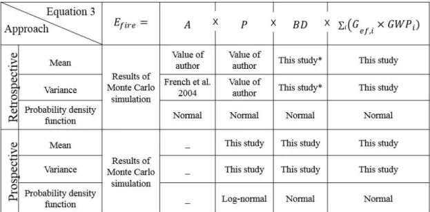
The second approach was a prospective approach. It consisted of making projections of future emissions by peat combustion. This approach also applies to the estimation of GHG emissions after a fire for which no measurement would have been taken. In this context, the depth of burn, bulk density and emission factors estimated in our meta-analyses can be considered as default values. The fire-damaged area was not used in this approach and the resulting estimated emissions were reported on a hectare basis. The sources of the parameters used to estimate GHG emissions according to both approaches are shown in Fig. 1-1.
2.5. Estimating and propagating uncertainty
The variance of GHG emissions can be estimated analytically using the (Goodman, 1960) formula (see Annex 1). According to this formula, the variance of the product of two random variables can be estimated as follows:
𝑉^(𝑥^ŷ) = 𝑥̂2𝑉^(ŷ) + 𝑦̂2𝑉^(𝑥^) − 𝑉^(𝑥^)𝑉^(ŷ) (1-6)
where 𝑉^ is the estimated variance and 𝑥^ and ŷ are the estimated parameters. Goodman's formula can easily be used recursively to provide an unbiased estimate of the variance for the estimated emissions (see Annex 2). Variance alone does not allow for confidence intervals and the distribution of the estimate is needed. In the context of this study, there is no certainty that the estimate of Lfire
follows a normal distribution. Indeed, although 𝑥^ and ŷ follow normal distributions, their product does not (Gaunt, 2018; Seijas-Macías & Oliveira, 2012).
In order to determine the distribution of the estimated GHG emissions, we carried out a Monte Carlo simulation with 100 000 runs (Tibshirani & Efron, 1993). Most parameters represented average values and, following the Central Limit theorem, it could reasonably be assumed that their estimates followed normal distributions (Casella & Berger, 2002).
The only exception was for the depth of burn in the prospective approach, which was assigned a log-normal distribution due to its heterogeneous variance (Fig. 1-1), as explained under Depth of burn in the Meta-analyses section.
Monte Carlo simulation was used in both the retrospective and prospective approaches. Realized parameters were drawn from probability density functions with the mean and variance as estimated through the meta-analyses, or as reported by the authors of the different studies (Fig. 1-1). The estimated fire-damaged area provided in each study was assumed to have a relative error of ±15 %, and to follow a normal distribution according to French et al. (2004). The estimated variance shown in Eq. 1-6 was used to validate the estimated variance we obtained from Monte Carlo simulation in
both approaches. The contribution of each parameter estimate to the total variance of estimated GHG emissions was assessed under both approaches using a correlation analysis between the realized parameters and the realized GHG emissions obtained from the Monte Carlo simulation.
Figure 1-1. Data organization to quantify GHG emissions according to each approach.
3. Results
3.1 Meta-analyses
The parameter estimates and their standard errors that were obtained from the meta-analyses are given in Table 1-4. The effect of land cover classification ("disturbed" versus "undisturbed") in the meta-analysis of bulk density was found to be non-significant with a p-value of 0.1161 and, consequently, this effect was not kept in the model. The sum of the emission factors for each GHG was estimated at 2,546 ± 75.32 kg Mg-1 of CO
2-eq. The contribution of the individual gas is shown in
Annex 3. Together, CO and CO2 amounted to 88 % of the total emissions, CH4 13% and NO -1 %.
Table 1-4. Parameter estimates and their standard errors obtained from the meta-analyses Parameter Estimate Standard error Std. deviation of random effects Std. deviation of residuals
Bulk density (Mg m-3) 0.145 0.018 0.040 0.10 Depth of burn (m) 0.228 0.1216 0.250* 0.98* Emission factors(kg Mg-1d.m) CO2 1,586.06 17.00 21.07 73.79 CH4 10.51 0.95 0.89 5.158 CO 258.68 15.34 24.40 46.41 NOx 1.04 0.47 0.78 0.36
3. Results
3.2. Estimated GHG emissions
3.2.1 Retrospective approach
Re-estimated GHG emissions with their respective confidence intervals for fire episodes between 1997 and 2015 are shown in Figs. 1-2 and 1-3. The fire episode in 1997 corresponds to the study by Page et al. (2002), the one in 2002 to Limin et al. (2004), the one in 2006 to Ballhorn et al. (2009), the one in 2015 to Simpson et al. (2016) and “Various” corresponds to the study by Konecny et al. (2016), which focused on the average of eight fires from 1997, 2001, 2002, 2004, 2005, 2006, 2009 and 2011.
In Fig. 1-2, the estimated GHG emissions are reported per hectare in order to facilitate their comparison. The fire episode of 1997 contributed most GHGs and displayed the largest confidence intervals. The fire episodes represented as “Various” contributed least and represented less severe fires on average.
Figure 1-2. Re-estimated greenhouse gas emissions based on the retrospective approach. The whiskers show the 0.95 confidence intervals obtained by Monte Carlo simulation. The labels 1997, 2002, 2006, 2015 and Various refer to the studies of each fire episode in the Table 1-1.
Figure 1-3. Distribution of the greenhouse gas emissions per hectare based on Monte Carlo simulation. The labels 1997, 2002, 2006, 2015 and various refer to the studies of each fire episode in the Table 1-1.
The contribution of each parameter to total variance is shown in Fig. 1-4. For all studies, the bulk density and fire-damaged area were the two major sources of uncertainty, followed by depth of burn and emission factors, for which the contributions were almost negligible in the study by Simpson et al. (2016) and Konecny et al. (2016) (Fig.1-4).
Figure 1-4. Contribution to variance of the different parameters in the re-estimated GHG emissions for the different fire episodes in the retrospective approach. The labels 1997, 2002, 2006, 2015 and various refer to the studies of each fire episode in the Table 1.
3. Results
3.2.2 Prospective approach
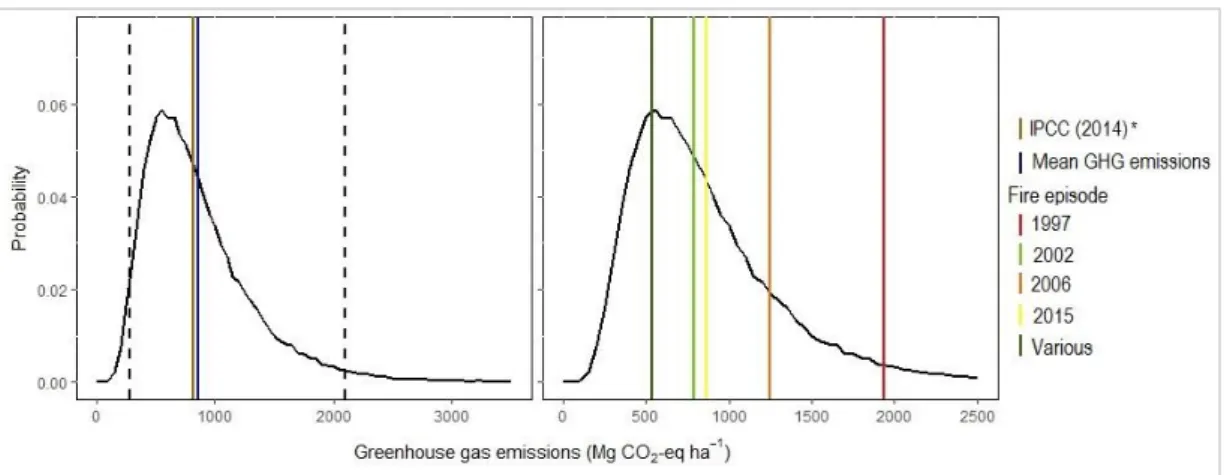
The GHG emissions for a future fire were estimated at 842 Mg ha-1 CO
2-eq. on average with a
standard deviation of 466 Mg ha-1 CO
2-eq. We obtained a 0.95 confidence interval ranging from 267
to 2 024 Mg ha-1 CO
2-eq. (Fig. 1-5). The mean predicted GHG emissions were very close to those
obtained with the IPCC guidelines (Hiraishi et al., 2014). The largest contribution to variance could be attributed to the depth of burn, with 94.2%, followed by bulk density with 5.5 % and the emission factor with 0.3 %. The difference between the variance estimated by Monte Carlo simulation and that obtained with Goodman's formula (Eq.1-6) did not exceed one percent, with the Monte Carlo variances and standard deviations always being greater (Table 1-5).
Figure 1-5. Distribution of GHG emissions from peat soil combustion in the prospective approach. Left: Mean GHG emissions estimated in the prospective approach and *mean estimated with default values provided by the IPCC (Hiraishi et al., 2014). The dashed lines represent the limits of the 0.95 confidence interval of the estimated GHG emissions in the prospective approach. Right: Means estimated in the retrospective approach for different fire episodes.
Table 1-5. Comparison of the relative standard deviations (%) estimated by Monte Carlo simulation with those estimated using Goodman’s estimator (Eq. 1-6).
Approach Fire episode Related study
Monte Carlo simulation
Goodman (1960)
Retrospective approach 1997 Page et al. (2002) 20.5 20.3
2002 Limin et al. (2004) 20.2 20.1 2006 Ballhorn et al. (2009) 21.6 21.2 2015 Simpson et al. (2016) 19.8 19.7 Various Konecny et al. (2016) 21.4 21.4