RESEARCH OUTPUTS / RÉSULTATS DE RECHERCHE
Author(s) - Auteur(s) :
Publication date - Date de publication :
Permanent link - Permalien :
Rights / License - Licence de droit d’auteur :
Institutional Repository - Research Portal
Dépôt Institutionnel - Portail de la Recherche
researchportal.unamur.be
University of Namur
Explaining African Growth Performance: A Production-Frontier Approach Houssa, Romain; Badunenko, Oleg; Henderson, Daniel J.
Publication date: 2010
Document Version
Early version, also known as pre-print
Link to publication
Citation for pulished version (HARVARD):
Houssa, R, Badunenko, O & Henderson, DJ 2010 'Explaining African Growth Performance: A Production-Frontier Approach'.
General rights
Copyright and moral rights for the publications made accessible in the public portal are retained by the authors and/or other copyright owners and it is a condition of accessing publications that users recognise and abide by the legal requirements associated with these rights. • Users may download and print one copy of any publication from the public portal for the purpose of private study or research. • You may not further distribute the material or use it for any profit-making activity or commercial gain
• You may freely distribute the URL identifying the publication in the public portal ? Take down policy
If you believe that this document breaches copyright please contact us providing details, and we will remove access to the work immediately and investigate your claim.
Explaining African Growth
Performance: A Production-Frontier
Approach
CRED WP 2010/13
Oleg Badunenko, Daniel J. Henderson, and Romain Houssa
Explaining African Growth Performance: A
Production-Frontier Approach
Oleg Badunenko
yDaniel J. Henderson
zRomain Houssa
xNovember 2010
Abstract
This paper employs a production frontier approach that allows distin-guishing technologic progress from efficiency development. Data on 35 African countries in 1970-2007 show that efficiency losses have constrained growth in Africa while technology progress has played a marginal growth enhancing role in the region. Moreover, physical and human capital accumulation are the main factors that drive productivity growth at the country level. Examing the outcomes of successful countries suggests that good governance, in-stitutional quality and good policies are key factors for improving economic development in Africa. These factors are even more required in Sub-Saharan Africa given the natural constraints of geography in the region.
The authors would like to acknowledge useful comments from participants of the 2010 African Economic Conference in Tunis, Tunisia.
yUniversity of Cologne, Cologne Graduate School in Management, Economics and Social
Sciences, Richard-Strauss-Str. 2, 50931, Cologne, Germany. Phone: +49.221.470.1285. Fax: +49.221.470.1229, E-mail: [email protected].
zDepartment of Economics, State University of New York, Binghamton, NY 13902-6000. Phone:
607-777-4480, Fax: 607-777-2681, E-mail: [email protected].
xUniversity of Namur, Centre of Research in the Economics of Development (CRED), Center
for Research in Finance and Management (CEREFIM), Rempart de la Vierge 8, B-5000 Namur, Belgium. Phone: +32.081 724 947. Fax: +32.081 724 840, E-mail [email protected].
1
Introduction
Over the past four decades the growth performance of Africa has been poor com-pared to that of other developing countries. In particular, the average African per capita real GDP growth has hardly surpassed two percent, while East Asia and Pacific countries have been experiencing impressive growth rates in the ranges of four to eight percent. Moreover, labor productivity did not change significantly and Sub-Saharan African (SSA) growth was even negative during the period start-ing from 1980 to the mid-1990s, whereas the growth of other low income coun-tries was well above zero in that period.1 This divergence of SSA growth is well documented as the “African growth tragedy” (see for exampleEasterly and Levine
(1997)).2
The poor African growth performance is worrisome given that the region needs to grow at a much higher level in order to meet the target for poverty reduction of the Millennium Development Goals (seeThe World Bank(2004)). A natural ques-tion thus emerges: why has Africa been growing so slowly whereas other regions have been achieving a sustained and higher level of growth?
This question has driven a large body of studies which broadly agree that low total factor productivity growth is the main impediment to the poor African growth performance (see for example Ndulu and O’Connell (1999), Ndulu and O’Connell (2009), Berthelemy and Söderling(2001), Hoeffler(2002), Fosu (2002),
Tahari et al.(2004)). While this literature has improved our understanding of the African growth tragedy, it fails to guide us directly to the factors behind the low productivity growth observed in SSA. The reason is that productivity cannot be viewed separately from development in technology and efficiency. As such, with-out a clear knowledge of the factor(s) responsible for low productivity growth, policy may be ineffective.
This study provides a comprehensive analysis of the African growth perfor-mance over the period 1970 to 2007. In particular, we use data from Penn World Tables (PWT) Version 6.3 in the framework ofHenderson and Russell(2005) to ex-amine the contribution of four factors to productivity growth in Africa: changes
1World Bank, World Development Indicators 2008 and African Development Indicators
2008-2009.
2Note thatBarro(1991) was the first to show the divergence of African growth with a
in efficiency, changes in technology and physical as well as human capital accu-mulation. More formally, we seek to address the following questions: What are the main impediments to economic growth in Africa? What characterizes the few successful African countries? Do African countries which are members of a mon-etary union, owing to market size and policy coordination, perform better than others? Do African countries that have improved macroeconomic management and institutional quality perform relatively better? Finally, what is the role of the abundance of natural resources in the African growth performance?
Our paper contributes to the existing literature in four ways. First, instead of analyzing the Solow residuals, loosely speaking, we decompose the Solow resid-ual into two components, which may not move in the same direction. We are thus able to isolate the contribution of technological change from that of efficiency in explaining the African evolution of productivity.
Second, we allow the technological changes to be non-neutral and analyze all African economies within a common production technology. This is in contrast with most of earlier studies that use the standard growth accounting approach where countries are analyzed separately. One benefit of our method is that we can better compare African countries and learn from success stories. For instance, our analysis should indicate whether successful African countries such as Botswana and Mauritius define the upper level of the African production frontier. More-over, our findings will indicate which of the four main determinants (physical and human capital accumulation, technological change and efficiency change) are the main drivers of growth in successful countries. It will also show us which factor(s) are the impediments in less successful countries.
Third, we pay special attention to the construction of human capital. In partic-ular, we estimate human capital similar to that inHall and Jones(1999). However, we use more recent and reliable data on school enrollment from Barro and Lee
(2010) together with estimates on returns to education which better suit African countries (Psacharopoulos and Patrinos (2004)). Most of the previous literature considers raw figures on school enrollment as a measure of human capital. While school enrollment would provide indication on the human capital stock, this mea-sure does not seem adequate to us in the African context.
Finally, we aim to identify and characterize the winners and the losers over our observed time period. Thus, we partition Africa according to various criteria
including geography, institutional framework, democracy, civil war and remote-ness. In particular, according to geography our grouping comprises North Africa (NA), SSA and its geographical subdivisions (West, East, South, costal opportu-nity, landlocked). In the same way, we use governance and political regime criteria to define Democracy and Autocracy. Other criteria allow us to consider the groups of Civil War, resource-rich and CFA countries.3 Our premise is that CFA members that are politically stable and African countries with a democratic regime will play an important role in the African growth recovery. On the other hand, we expect that countries that experienced civil wars and other armed conflicts will perform poorly.
2
Data
We derive data for 35 African countries from the Penn World Tables (PWT), Ver-sion 6.3. The number of workers is obtained as RGDPCH * POP/RGDPWOK, where RGDPCH is per capita GDP computed via the chain method, POP is the population and RGDPWOK is real GDP per worker. The measure of output is cal-culated as RGDPWOK multiplied by the number of workers; the resulting output is in 2005 international dollars. Real aggregate investment in 2005 international dollars is computed as RGDPL * POP * KI, where RDGPL is the real GDP com-puted via the Laspeyres index, and KI is the investment share of real GDP. We apply the perpetual inventory method (PIM) to the real investment series to con-struct the physical capital stock. More specifically, the current capital stock is the sum of the current investment and depreciated capital stock from the previous period. Following standard practice, we compute the initial capital stock, K0, as
I0=(g + ), where I0is the value of the investment series in the first year it is
avail-able, and g is the average geometric growth rate for the investment series between the first year with available data and 1980 (Caselli and Feyrer(2007)).
For human capital, we employ the Barro and Lee(2010) education data. The data are available every five years and we linearly extrapolate the data to obtain
3The CFA franc Zone is a monetary Union that includes 14 SSA countries: Benin, Burkina Faso,
Cameroon, Central African Republic, Congo Republic, Cote d’Ivoire, Equatorial Guinea, Gabon, Guinea Bissau, Mali, Niger, Senegal, and Togo. The currency of the union was pegged to the French franc before 1999 and now to the Euro. For details on institutional features on the CFA zone seeFielding(2005).
values in between. These education data are an update of widely used previous compilation of Barro and Lee (2001). Using the improved data, we follow HR and adopt the Hall and Jones (1999) construction of human capital. However, instead of using the Psacharopoulos (1994) survey of wage equations to evalu-ate the returns to education, we use Psacharopoulos and Patrinos (2004) which provide a more comprehensive study of the returns to education in Africa. Ta-ble A1 of Psacharopoulos and Patrinos (2004) provides country specific returns to education for various African economies at different years. To make unified and general conclusions, we average the returns for each level of education for the African countries given in their table and apply them to all countries in our sample to construct our human capital measure. Specifically, let jtrepresents the
average number of years of education of the adult population in country j at time tand define labor in efficiency units in country j at time t by
^
Ljt = HjtLjt = h( jt)Ljt = exp (jt)Ljt; (1)
where is a piecewise linear function, with a zero intercept and a slope of 0.266 through the sixth year of education, 0.173 for the next six years, and 0.113 for education beyond the twelfth year. Clearly, the rate of return to education (where
is differentiable) is @ ln h( jt) @ jt = 0( jt) (2) and h(0) = 1.
3
Methodology
3.1
Data Envelopment Analysis
We follow the methodology ofHenderson and Russell(2005) to construct country-specific production frontiers and retrieve efficiency scores. More country-specifically, we use a nonparametric approach to efficiency measurement, Data Envelopment Analy-sis, which rests on assumptions of free disposability to envelope the data in the smallest convex cone, the upper boundary of which is the “best-practice” frontier. The distance from an observation to such cone then presents measure of technical
efficiency. Data Envelopment Analysis is a data driven approach in the sense that it allows data to tell where the frontier lies without prior specifying the functional form of the technology (seeKneip et al. (1998) for a proof of consistency for the DEA estimator, as well asKneip et al.(2008) for its limiting distribution).
We specify technology to contain four macroeconomic variables: aggregate output and three aggregate inputs—labor, physical capital, and human capital. Let hYit; Kit; Lit; Hiti, t = 1; 2; : : : ; T , i = 1; 2; : : : ; N, represent T observations on
these four variables for each of the N regions. We adopt a standard approach in the macroeconomic literature and assume that human capital enters the tech-nology as a multiplicative augmentation of physical labor input, so that our N T observations are hYit; Kit; ^Liti, t = 1; 2; : : : ; T , i = 1; 2; : : : ; N, where ^Lit = LitHit
is the amount of labor input measured in efficiency units in region i at time t. The constant returns to scale technology in period t is constructed by using all the data up to that point in time as
Tt= 8 > < > : D Y; ^L; KE2 <3+j Y P t P i zi Yi ; ^L P t P i zi L^i ; K P t P i zi Ki ; zi 08 i; 9 > = > ;; (3)
where zi are the activity levels. Notice that we have two separate summations.
The latter refers to the country while the former refers to time. Here the summa-tion is over t. This implies that when calculating the technology in period t, the previous years technology are also available. That is, it is assumed that tech-nologies available in previous years were not lost and were at disposal in later years. Indeed, we believe that it is reasonable to assume that in period t coun-try i is able to employ the technology that it has been using in previous periods. That being said, there is no reason to believe it is necessarily efficiently using past technologies.
TheFarrell(output-based) efficiency score for region i at time t is defined by E(Yit; ^Lit; Kit) = min n j DYit= ; ^Lit; Kit E 2 Tt o : (4)
This score is the inverse of the maximal proportional amount that output Yit can
be expanded while remaining technologically feasible, given the technology and input quantities. It is less than or equal to unity and takes the value of unity if and
only if the it observation is on the period-t production frontier. In our special case of a scalar output, the output-based efficiency score is simply the ratio of actual to potential output evaluated at the actual input quantities.
3.2
Quadripartite Decomposition
We again follow the approach ofHenderson and Russell(2005) to decompose pro-ductivity growth into components attributable to (1) changes in efficiency (techno-logical catch-up), (2) techno(techno-logical change, (3) capital deepening (increases in the capital-labor ratio), and (4) human capital accumulation. Under constant returns to scale we can construct the production frontiers in ^y ^kspace, where ^y = Y = ^L and ^k = K= ^L are the ratios of output and capital, respectively, to effective la-bor. Letting b and c stand for the base period and current period respectively, the potential outputs per efficiency unit of labor in the two periods are defined by yb(^kb) = ^yb=eb and yc(^kc) = ^yc=ec, where eb and ec are the values of the efficiency
scores in the respective periods as calculated in Eq. (4) above. Hence, ^ yc ^ yb = ec eb yc(^kc) yb(^kb) : (5)
Let ~kc = Kc=(LcHb)denote the ratio of capital to labor measured in efficiency
units under the counterfactual assumption that human capital had not changed from its base period and ~kb = Kb=(LbHc) the ratio of capital to labor measured
in efficiency units under the counterfactual assumption that human capital were equal to its current-period level. Then yb(~kc)and yc(~kb)are the potential output per
efficiency unit of labor at ~kc and ~kb using the base-period and current-period
tech-nologies, respectively. By multiplying the numerator and denominator of Eq. (5) alternatively by yb(^kc)yb(~kc)and yc(^kb)yc(~kb), we obtain two alternative
decompo-sitions of the growth of ^y ^ yc ^ yb = ec eb yc(^kc) yb(^kc) yb(~kc) yb(^kb) yb(^kc) yb(~kc) ; (6)
and ^ yc ^ yb = ec eb yc(^kb) yb(^kb) yc(^kc) yc(~kb) yc(~kb) yc(^kb) : (7)
The growth of productivity, yt = Yt=Lt, can be decomposed into the growth of
output per efficiency unit of labor and the growth of human capital, as follows: yc yb = Hc Hb ^ yc ^ yb : (8)
Combining Eq. (6) and (7) with (8), we obtain yc yb = ec eb yc(^kc) yb(^kc) yb(~kc) yb(^kb) " yb(^kc) yb(~kc) Hc Hb # (9) EF F T ECHc KACCb HACCb;
and yc yb = ec eb yc(^kb) yb(^kb) yc(^kc) yc(~kb) " yc(~kb) yc(^kb) Hc Hb # (10) EF F T ECHb KACCc HACCc:
Eq. (9) and (10) decompose the growth of labor productivity in the two periods into changes in efficiency, technology, the capital-labor ratio, and human capital accumulation. The decomposition in Eq. (6) measures technological change by the shift in the frontier in the output direction at the current-period capital to effective labor ratio, whereas the decomposition in Eq. (7) measures technological change by the shift in the frontier in the output direction at the base-period capital to effective labor ratio. Similarly, Eq. (9) measures the effect of physical and human capital accumulation along the base-period frontier, whereas Eq. (10) measures the effect of physical and human capital accumulation along the current-period frontier.
These two decompositions do not yield the same results unless the technology is Hicks neutral. In other words, the decomposition is path dependent. This am-biguity is resolved by adopting the “Fisher Ideal” decomposition, based on geo-metric averages of the two measures of the effects of technological change, capital
deepening and human capital accumulation and obtained mechanically by multi-plying the numerator and denominator of Eq. (5) by yb(^kc)yb(~kc)
1=2 yc(^kb)yc(~kb) 1=2 : yc yb
= EF F (T ECHb T ECHc)1=2 (KACCb KACCc)1=2 (HACCb HACCc)1=2
EF F T ECH KACC HACC: (11)
3.3
Distribution Analysis
Our distribution analysis exploits the quadripartite decomposition of the produc-tivity growth and examines the impact of each of the four components on the transformation of the productivity distribution over time. By following the idea ofHenderson and Russell(2005) we rewrite the decomposition in Eq. (11) so that the labor productivity distribution in the current period can be constructed by consecutively multiplying the labor productivity in the base period by each of the four components:
yc = (EF F T ECH KACC HACC) yb: (12)
To study the effect of a given component, we isolate its impact by construct-ing a counterfactual distribution introducconstruct-ing only this component. Accordconstruct-ingly, the compound effect of two components is isolated by creating a counterfactual distribution introducing these two components, etc. For example, we investigate the unique effect of capital deepening on the labor productivity distribution in the base period assuming no efficiency, technological change, or human capital accumulation by looking at the distribution of the variable
yK = KACC yb: (13)
By the same token, assuming further no technological change or human capital ac-cumulation, we examine the compound effect of capital deepening and efficiency change on the labor productivity distribution in the base period by constructing the counterfactual distribution of the variable
Assuming further no technological change, we are able to isolate the effect of capi-tal deepening, efficiency change, and human capicapi-tal accumulation by focusing on the counterfactual distribution of the variable
yKEH = (KACC EF F HACC yb) = HACC yKE: (15)
It is evident that multiplying the distribution of yKEHby the effect of technological
change yields the labor productivity distribution in the current period allowing us to assess the effect of all four components. The choice of the sequence in which components are introduced in Eq. (13) (15) is arbitrary and depends on the focus of the analysis on the effect(s) of particular component(s).
4
Empirical Results
4.1
Efficiency Scores
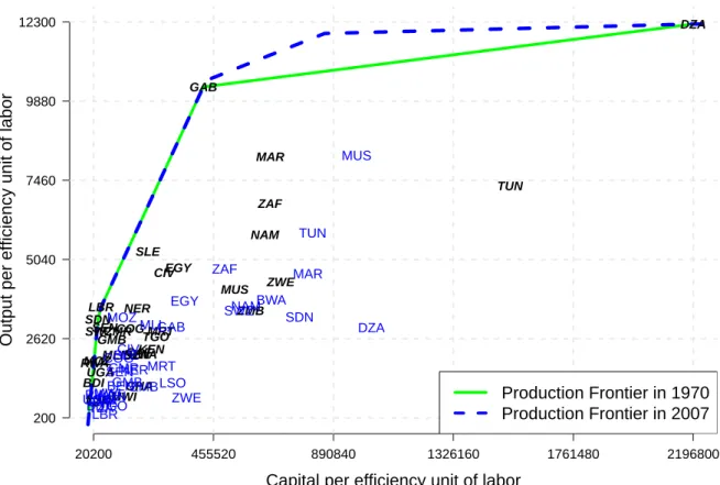
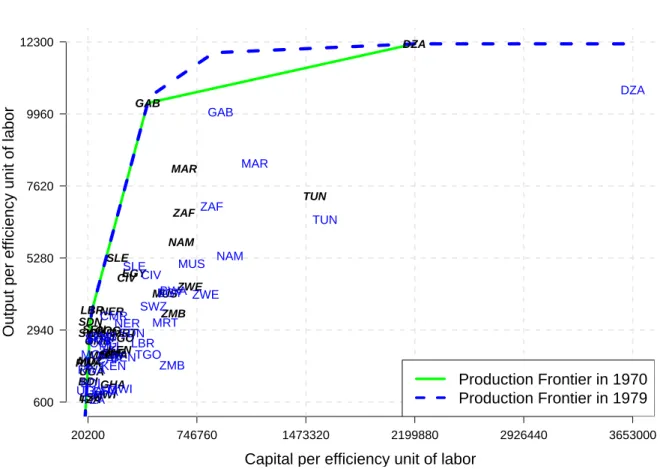
Figure 1 presents observations of African economies in 1970 and 2007, and also superimposes the production frontiers for 1970 and 2007. The first year in our sample is 1970 and hence we construct the 1970 frontier using solely these points. However, for the 2007 frontier, in addition to the data from 2007, we also include both the inputs and output for each country from 1970-2006. By doing so, we let countries in 2007 use technologies which were available in each year prior to 2007. Allowing for this means that the 1970 observations of Algeria, Gabon, Liberia, and Sudan as well as the 1971 and 1976 observations of Gabon define the frontier in 2007.4
The fact these countries in previous time periods define the 2007 frontier may sound surprising to some, but to those familiar with African growth, these re-sults should be expected. For example, consider the case of Gabon which defines the 2007 frontier in three of its past periods. In the 1960s and 1970s Gabon en-joyed economic prosperity thanks to its natural resources such as timber (forest occupies about 85% of the surface), manganese and uranium. Moreover, although
4In order to ensure that countries defining the frontier are not key to our results, we also
re-moved them from the sample and ran the results again. The results remain qualitatively similar and are available from the authors upon request.
Gabon initiated oil extraction in 1956, it became important in the 1970s after oil offshore discoveries and the first oil shocks of that period. In 1975, oil produc-tion reached a record high of 225000 barrels per day and Gabon joined OPEC. As such, Gabon’s revenue increased tremendously following the oil price shocks of the 1970s. Moreover, given the relatively small size of the population (about 1 mil-lion inhabitants), civil servants in Gabon were among the highest paid in Africa and this factor fueled consumption.
We should also discuss the case of Algeria. Algeria gained its independence from France in 1962. The French occupation went back to the 1800s. France put in place various infrastructures such as roads, railroads, bridges and harbors. They also modernized the agriculture, industrial, health and education sectors. During French domination, the settlers also made successful campaigns against diseases such as malaria (Acemoglu et al.(2001)). As such, it is not surprising that Algeria had the lowest mortality rate in Africa in the colonial period and Algeria also had the highest percentage rate of settlers in Africa (Acemoglu et al.(2001)). Given the precedent, it is not surprising that income per capita was 60 percent higher in Algeria compared to other NA countries such as Tunisia in 1960 (Chemingui and El-Said. (2007)). Note that Algeria had large oil and gas revenues and this may have contributed substantially to defining the frontiers. Algeria is the fourth largest African oil producer after Nigeria, Angola, and Libya. Moreover, Algeria is the sixth largest natural gas producer in the world after Russia, the United States, Canada, Iran, and Norway.
Finally, consider the case of Liberia. The colonial history of Liberia is very different from other African countries. In particular, while all others have been colonized by Europeans, Liberia was founded and colonized by American freed slaves. As such, Liberia has historical ties with the USA. The support and presence of Americans in Liberia may have induced the settlement of good institutions and infrastructures and could explain why Liberia may be more efficient than other countries and defines the frontier in 1970. The country enjoyed political stability for a long period and was modeled on the American style. This has also contributed to stable economic growth in the country. The main sources of income were mining of or iron. Ties links with the USA also encouraged FDI inflows to the country.
Turning back to the Figure 1, we see that up to a capital per efficiency unit of labor ratio around 400; 000 (Gabon in 1970), the production frontiers in 1970 and
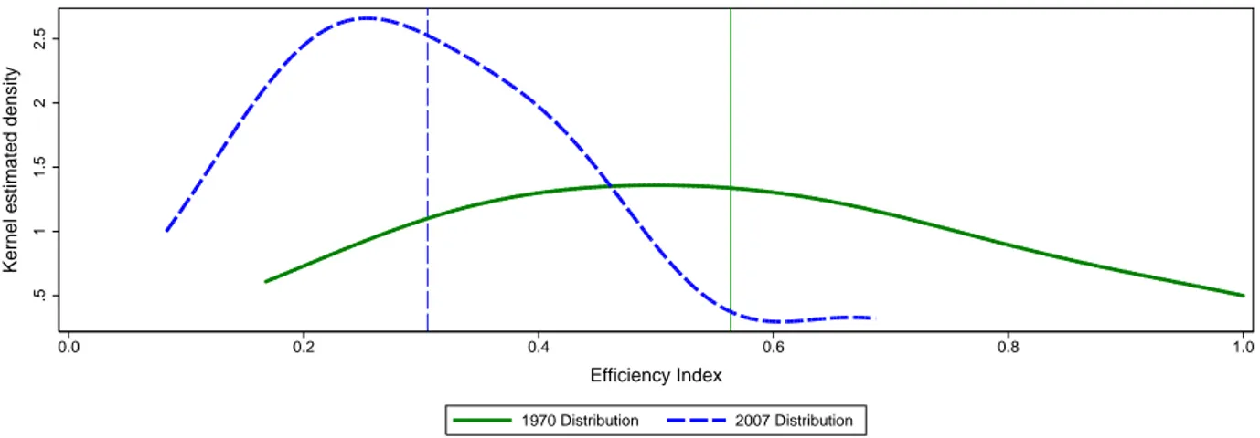
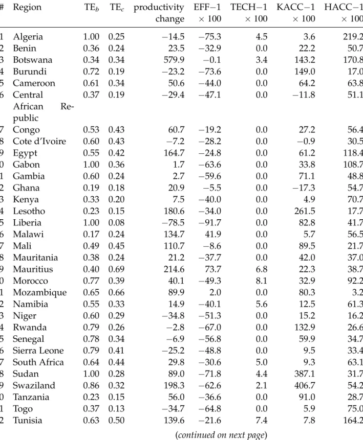
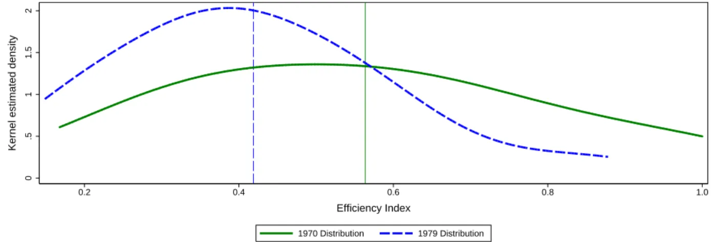
2007 are identical. Starting from this capital to efficient unit of labor ratio, the 2007 frontier shifts upward. In particular, the shift induces a gap between the two fron-tiers which widens until a capital per efficiency unit of labor ratio value of about 850; 000(Gabon in 1976) from which the gap starts shrinking until the two fron-tiers equalize at the highest level of capital ratio of around 2; 000; 000 (Algeria in 1970). This trend in the two frontiers suggest that the main technological changes occur in countries with a capital per efficient unit of labor ratio in excess of 455520. Recall that the distance from the frontier (in the output direction) determines the efficiency of each country. Figure 2 presents distributions of the efficiency indexes in 1970 and 2007. The data show an important shift of the distribution away from the frontier between 1970 and 2007. This observation suggests that African economies have become less efficient between 1970 and 2007. The second and third columns of Table 1, which give the efficiency scores for each country in 1970 and 2007, confirm this finding. This trend in the distribution of efficiency in African countries is troublesome because their level of efficiency was already low in 1970. In particular, the data in Table 1 show that the potential gains from removing inefficiency in African countries are enormous—up to 44 (69) percent on average in 1970 (2007). Notice that the mean weighted (by population) aver-age efficiency index (last row of Table 1) is not very different than its counterpart unweighted average. This result implies that the (population) size of countries is not determining their technical efficiencies.
Related to this latter point and as one might expect, the performance of ef-ficiency is fairly heterogeneous across African countries. However, interesting results can be derived from averages across predefined groups reported in Table 2.5 For instance, looking at the results across geographical areas shows that NA is much more efficient than SSA. This result could be explained by fundamental differences between the two regions. In particular, disease burdens of malaria and HIV and the exposure to rainfall shocks are among documented constraints to economic development in SSA (see Gallup et al. (1999) and Artadi and Sala-i Martin(2003)). Intuitively, diseases reduce returns on FDI and raise transaction costs on international trade, migration, and tourism. As such, they reduce the op-portunity to learn from developed countries (Gallup and Sachs(2001)). Moreover, geographical constraints may affect the choice of economic policy in SSA. Indeed, in an environment where few firms operate because of high costs, the revenue
maximizing tax policy of the government is to impose high taxes on economic activity which further reduces firms efficiency (see Collier and Gunning (1999) and Gallup and Sachs (2001)). Finally, agriculture productivity should be lower in SSA than in NA because the former has a tropical climate while the latter has a temperate-zone climate (seeBloom and Sachs(1998) andPorter(1995)).
Another difference between the two regions that could explain this gap is the type of redistributive norm in place in each region. The redistributive norm in SSA is such that successful individuals have the obligation to share their wealth with extended family members and others in the community (seePlatteau(2000),
Platteau (2009) and Platteau (2010)). There are several possible impacts of such norms on efficiency and economic development in general (seePlatteau(2010) for a nice exposition). For example, such norms discourage effort because the mar-ginal productivity of effort is shared among many people while the cost of effort is only taken by one person. Also, such redistributive pressures discourage saving, investment, entrepreneurship and risk taking because the risk taker will only face the cost when the project fails, while they will have to share the benefit when the project succeeds. It also encourages a misallocation of resources. In particular, in such an environment, a manager is pushed to hire his friends and relatives even if they do not have the right qualifications. A final example is that these norms en-courage people to hide their wealth. Using survey data from rural creditBaland et al. (forthcoming) find excess borrowing behavior in Cameroon. In particular, they report that more than 20 percent of loans are fully collateralized by liquid savings of the cooperative members. Moreover, they find that the amount of bor-rowers’ liquid savings is on average the double of that of the loan they obtained. This practice is inefficient because the interest rate on credit is much higher than that on deposit. However, “those interviews indicate that some members system-atically use credit as a way to pretend that they are too poor to have available savings. By doing so, they can successfully oppose request for financial help from friends and relatives”.
Other groupings are also interesting. Consistent with these factors, our re-sults indicate that landlocked African countries are less efficient than their coastal counterparts. However, this result is not true in 1970. One explanation why costal countries were less efficient than their landlocked counterparts could be that the former was more exposed to the slave trade that weakened the development of economic activities (seeNunn(2008) for the arguments). However, as we entered
into the globalization period, the costal countries became relatively more efficient because of their low cost for trade and FDI. This result is confirmed by sub-period analysis over four decades between 1970 and 2007 (see our appendices).
Comparing the results across SSA shows that CFA country members are more efficient than the rest. The fundamental difference between the two groups are that CFA members have belonged to a monetary union for about half a century. This framework has imposed monetary and fiscal policy discipline on CFA mem-bers. As such, these countries enjoyed low levels of inflation and inflation volatil-ity as compared to others in SSA (see Bleaney and Fielding (2002) and Houssa
(2008)). Another interesting result in Table 2 is that in 1970, resource rich coun-tries are more efficient, especially the Northern councoun-tries. This result is consistent with our analysis of countries that define the production frontier. In particular, a large part of FDI inflows to Africa are directed to the natural resource sector. Therefore, ceteris paribus, countries with abundant natural resources which at-tract more FDI, may also atat-tract better managerial techniques and would be rela-tively more efficient.
4.2
Productivity Growth
The third column of numbers in Table 1 presents the growth of labor productiv-ity. During some thirty years under consideration, labor productivity increased by 54 percent on average (unweighted). The productivity gains, however, are dis-tributed unevenly (see Table 1). In particular, Table 2 shows that countries with a democratic regime, those located in Southern Africa and those in costal areas are the biggest winners in terms of labor productivity between 1970 and 2007. Within these groups, we observe an impressive productivity improvement in Botswana, Mauritius, Malawi, Mozambique, Lesotho, and Swaziland. On the other side, West Africa is the only group for which labor productivity has decreased between 1970 and 2007. This result may capture the adverse effects of drought in Niger and Senegal. Moreover, the results reflect the low performance of countries that have experienced political instability, civil wars and other armed conflicts in the region: Cote d’Ivoire, Liberia, Sierra Leone, and Togo. In general, our results are consis-tent with the literature that armed conflicts and civil wars destroy and discourage physical and human capital accumulation, but also lead to the misallocation of resources (see Baland et al. (2010), Collier (1999), Collier and O’Connell (2009),
Ngaruko and Nkurunziza (2009), and Imai and Weinstein (2000)). Algeria and Liberia, two countries that defined the African efficiency frontier in 1970, experi-enced huge losses in efficiency following political instability in the 1980s and the civil wars in the 1990s in Liberia and political instability and armed conflicts in the early 1990s in Algeria. Moreover, the results show physical capital depletion in these countries in the 1980s and 1990s (see the appendices for decade-wise re-sults). Similar results hold true for other countries such as Burundi, Rwanda and Sierra Leone.
4.3
Quadripartite Decomposition
The contributions to changes in efficiency, technological change, capital deepen-ing, and human capital accumulation are presented in the last four columns of Table 2. It is clear that physical and human capital accumulation are the factors that drive productivity growth at the country level. However, given diminish-ing return to capital, this result may explain why constant growth has not been sustainable in Africa.
Although most countries are driven by physical and human capital accumula-tion, some countries have also benefited from technological change. In particular, apart from Egypt, all NA countries have improved their level of technology be-tween 1970 and 2007. It is possible that this result reflects the geographical prox-imity of NA to Europe. Technological catch up also occurred in Southern African for countries such as Botswana, Mauritius, Namibia, and South Africa.
Efficiency improvements have helped to increase productivity only in Malawi, Mauritius and Mozambique. In all other cases, it impeded the productivity growth and did so to a large extent. This result suggests that improving efficiency in Africa is very important to generate sustained growth. In addition, the results show that Mauritius is the only country that has gained in all four factors during the 1970-2007 period. This finding is consistent with the widely held view that Mauritius is a successful African story. This success story deserves particular at-tention because initial conditions were relatively poor in Mauritius. Mauritius has no mineral resources and sugar cane was the main driver of income through its independence in 1968. This single good based economy made the country vul-nerable to terms of trade shocks, but also to rainfall related conditions. In the
1960s and 1970s, the country also experienced rapid population growth and eth-nic conflicts. As such, Mauritius had very poor initial economic conditions even compared to other African nations.6 This finding is also consistent with our esti-mated efficiency scores in Table 1, showing that Mauritius was less efficient than the average African country in 1970. These weak initial conditions in Mauritius led some economists conclude that the country would fail to develop (seeMeade
(1961),Meade(1967) andMeade et al.(1961)).
Following the Meade et al.(1961)’s report, the government of Mauritius em-barked on a number of industrialization policies in the 1960s. The context was characterized by the Import Substitution Investment (ISI) development strategy. In this framework, Mauritius initiated the creation of manufacturing firms tar-geted towards food processing, beverages, cosmetics, fertilizers, footwear, furni-ture and paints in 1963. These firms were protected against foreign competition with tariff and import quotas. Moreover, the Mauritian Investment bank was cre-ated in 1964 in order to ease financing of the newly established firms. In 1968, Mauritius initiated an Export Processing Zone (EPZ). The key motivation of this policy was to gain export market access and complement the ISI supported firms that were only producing for the domestic economy. EPZ is a package of trade lib-eralization policies aiming to attract FDI and to gain access to the export market. As such, a number of studies argue that trade openness and FDI inflows have been the main drivers of growth in Mauritius (seeRomer(1992),Sachs et al.(1995) and
Sachs and Warner(1997)). Intuitively, through trade and FDI, the domestic econ-omy imports better technologies and managerial techniques but also new ideas. As a result, access to trade and FDI improves technology and efficiency and in turn becomes more productive.
We should note, however, that EPZ policies did not succeed in other African countries. For instance, Senegal introduced EPZ in 1974, Liberia in 1975, Cote d’Ivoire in 1976, Togo in 1977, and the Democratic Republic of Congo in 1978. One explanation to the success of the EZP program in Mauritius versus the others may have to do with the different institutional framework and the set of policies that were implemented in each of these countries. Rodrik (1998) argues that the im-plementation of a heterodox trade liberalization policy has been the determinant
6Note, however, that Mauritius had initially a better human capital level than other nations in
Africa. In particular, life expectancy was about 60 years in Mauritius in the 1970s compared to only 42 years for others.
for the success of EPZ in Mauritius. This heterodox policy involves asymmetric trade policies across imports and exports. In particular, Mauritius removed taxes on inputs needed for the development of the export sector. At the same time, the ISI was still effective on other imported goods. As such, the export sector did not suffer from anti-export bias of ISI. In addition, Mauritius has had a better macro-economic environment than other African nations. For instance, Mauritius has had a relatively lower inflation level. Moreover, and most importantly, exchange rate policies of the country had delivered undervalued exchange rates such as to obtain competitiveness to exporting firms (Prasad et al. (2007)). In light of these considerations,Subramanian(2009) claims that better the institutional framework has been the main factor behind Mauritius’ EPZ success. Indeed, theRotberg and Gisselquist(2009) African index of governance ranks Mauritius with the best per-formance since 2000. The country has also constantly enjoyed democracy for the last 40 years. With better governance put in place in Mauritius, there is relatively limited room for corruption and therefore a relatively better business environ-ment to attract productive investenviron-ment.7 It is no surprise that Mauritius is the first African country to be ranked in the top 20 in the world of the World Bank doing business report for 2010.
Partially driven by Mauritius, Table 2 shows that countries with a democratic regime have much better performance than any other group.8 In this vein, Botswana and Malawi also display a strong performance owning to their better institutional quality (seeAcemoglu et al. (2002) andNdulu and O’Connell (1999)). However, Botswana has seen a number of challenges such as the development of HIV in the 1990s and rising unemployment.
Finally, note that the international environment has been favorable to the suc-cess of EPZ in Mauritius. In particular, Mauritius has benefited from preferential trade treatments from the developed world. For instance, Mauritius has been ex-empted from protectionism trade policies from the EU and USA. This exemption was clearly a subsidy to the EZP sector in Mauritius. Such a favorable treatment may not be available today for other developing countries. Moreover, globaliza-tion has made export market access today more difficult for developing countries.
7Gyimah-Brempong and de Gyimah-Brempong(2006) recently find that corruption has a larger
detrimental impact in Africa than in other regions of the world.
8We use the Polity IV data whose values range from -10 (autocracy) to +10 (democracy).
More-over, we follow the database and concentrate on two groups of countries: i) democracies with scores in the ranges +6 to 10; and ii) autocracies and anocracies for others.
In light of this consideration,Collier(2008) observes that least developing coun-tries will find it more difficult today to replicate the Mauritian EPZ success. That being said, EPZ still succeeded in Mauritius while it failed in other SSA countries that introduced the framework in a similar period to Mauritius. Moreover, Mau-ritius managed successfully the benefits from EPZ success. For instance, revenues derived from EPZ have been invested in the service sector which accounts today for nearly 70 percent of its economy compared to less than 5 percent in the early 1970s.
4.4
Productivity Distributions
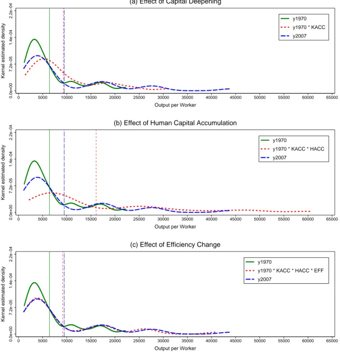
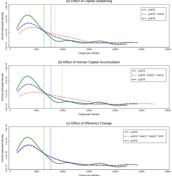
The solid and dashed lines in each panel of Figure 3 are the distributions of output per worker in 1970 and 2007. The figure suggests that the shape of the distribu-tion has somewhat changed. The ‘poor’ mode has less mass in 2007 which implies that fewer countries are poor. As the richer countries became even wealthier, the right tail of the blue dashed distribution stretched to higher levels of output per worker, providing some evidence for a widening income gap between rich and poor regions. However, theLi (1996) test provides no evidence that the two dis-tributions are statistically significantly different from each other. One explanation may be that there are not enough points in each year to statistically distinguish the two curves. If this is not the case, then this says that there has been no change in nearly 40 years. This stagnation is disheartening.
The counterfactual distributions also appear in Figure 3. Panel (a) shows the isolated effect of physical capital accumulation. Physical capital accumulation, by itself, has made relatively poorer countries richer and moved the original 1970 output worker distribution closer to that of 2007. Recall that it is poorer countries that benefited more from capital deepening. Human capital accumulation moved the output per worker distribution even further to the right (panel (b)), thus mak-ing each country richer. It should be noted that relatively richer countries got more from the accumulation of human capital. Panel (c) suggests that efficiency change has moved the whole distribution leftward, thus eroding the positive ef-fects of factor accumulation. It is here where African countries should focus their attention. Finally, the difference between the dotted and dashed curves in panel (c) is the effect of technological change. Although we have seen that
technolog-ical change had positive effect for some countries, it does not appear to shift the distribution at all.
5
Concluding Remarks
Studying growth patterns and determinants of African economies is essential for understanding what can be done to reduce the gap between the performance of the continent and the rest of the world. Instead of having the African continent as a separate group and comparing its average performance to the other regions in the world, we decide to make a cross-African analysis where we benchmark African economies against one another. Additionally, in order to draw valid con-clusions, we employ robust and advanced methodologies to the most reliable data we could obtain. To the best of our knowledge, this paper is the first attempt to address each of these challenges. First, we gather reliable data on 35 African economies. Second, we pay special attention to constructing a reliable measure of the human capital. Third, we apply an advanced methodology. Specifically, we analyze labor productivity growth by decomposing it into four components at-tributable to efficiency change, technological change, physical and human capital accumulation.
We find that physical and human capital accumulation are the factors that drive productivity growth at the country level for all countries considered. Di-minishing marginal returns hence partially explain why Africa (as a whole) has failed to generate sustained growth. Moreover, efficiency losses have constrained growth in Africa. Examining the outcome in successful countries, such as Mauri-tius and Botswana, suggests that good governance, institutional quality and good policies are key factors to improve economic development in Africa. These factors are even more required in SSA given the natural constraints of geography of the region.
References
Acemoglu, D., Johnson, S. and Robinson, J. A.: 2001, The colonial origins of com-parative development: An empirical investigation, American Economic Review
91(5), 1369–1401.
Acemoglu, D., Johnson, S. and Robinson, J. A.: 2002, An african success story: Botswana, CEPR Discussion Papers 3219, C.E.P.R. Discussion Papers.
Artadi, E. and Sala-i Martin, X.: 2003, The economic tragedy of the XXth century: Growth in africa, NBER Working Papers 9865, National Bureau of Economic Re-search.
Baland, J.-M., Guirkinger, C. and Mali, C.: forthcoming, Pretending to be poor: borrowing to escape forced solidarity in Cameroon, Economic Development and Cultural Change .
Baland, J.-M., Moene, K.-O. and Robinson, J. A.: 2010, Governance and develop-ment. CRED WP 2010/07.
Barro, R. J.: 1991, Economic growth in a cross section of countries, The Quarterly Journal of Economics 106(2), 407–43.
Barro, R. J. and Lee, J.-W.: 2001, International data on educational attainment: Updates and implications, Oxford Economic Papers 53(3), 541–563.
Barro, R. J. and Lee, J.-W.: 2010, A new data set of educational attainment in the world, Working Paper 15902, National Bureau of Economic Research.
URL: http://www.nber.org/papers/w15902
Berthelemy, J.-C. and Söderling, L.: 2001, The role of the capital accumulation, adjustment and structural change for economic take-off : Empirical evidence from African growth episodes, World Development 29, 323–343.
Bleaney, M. and Fielding, D.: 2002, Exchange rate regimes, inflation and output volatility in developing countries, Journal of Development Economics 68(1), 233– 245.
Bloom, D. E. and Sachs, J. D.: 1998, Geography, demography, and economic growth in Africa, Brookings Papers on Economic Activity 29(2), 207–296.
Caselli, F. and Feyrer, J.: 2007, The marginal product of capital, Quarterly Journal of Economics 122(2), 535–568.
Chemingui, M. and El-Said., M.: 2007, Algeria’s macroeconomic performance from 1962 to 2000, Explaining Growth in the Middle East, Contributions to Economic Analysis, Vol. 278 J. Nugent and H. Pesaran, eds., Amsterdam: Elsevier.
Collier, P.: 1999, On the economic consequences of civil war, Oxford Economic Paper
51(1), 168–183.
Collier, P.: 2008, The bottom billion: why the poorest countries are failing and what can be done about it., Oxford University Press.
Collier, P. and Gunning, J. W.: 1999, Why has Africa grown so slowly?, Journal of Economic Perspectives 13(3), 3–22.
Collier, P. and O’Connell, S. A.: 2009, Opportunities, episodes, and syndromes, in B. J. Ndulu, S. A. O’Connell, R. H. Bates, P. Collier and C. C. Soludo (eds), The Political Economy of Economic Growth in Africa, 1960–2000, Vol. 1 of Cambridge Books, Cambridge University Press.
Easterly, W. and Levine, R.: 1997, Africa’s growth tragedy: Policies and ethnic divisions, The Quarterly Journal of Economics 112(4), 1203–1250.
Farrell, M. J.: 1957, The measurement of productive efficiency, Journal of the Royal Statistical Society. Series A (General) 120(3), 253–290.
Fielding, D.: 2005, Macroeconomic policies in the Franc Zone, Palgrave Macmillan, Basingstoke.
Fosu, A. K.: 2002, Political instability and economic growth: Implications of coup events in Sub-Saharan Africa, American Journal of Economics and Sociology
61(1), 329–348.
Gallup, J. L. and Sachs, J. D.: 2001, The economic burden of malaria, American Journal of Tropical Medicine and Hygiene 64(1-2), 85–96.
Gallup, J., Sachs, J. and Mellinger, A.: 1999, Geography and economic develop-ment, in S. J. Pleskovic B (ed.), Annual Conference on Development Economics, Washington, DC: World Bank.
Gyimah-Brempong, K. and de Gyimah-Brempong, S.: 2006, Corruption, growth, and income distribution: Are there regional differences?, Economics of Gover-nance 7(3), 245–269.
Hall, R. E. and Jones, C. I.: 1999, Why do some countries produce so much more output per worker than others?, Quarterly Journal of Economics 114(1), 83–116. Henderson, D. J. and Russell, R. R.: 2005, Human capital and convergence: A
production-frontier approach, International Economic Review 46(4), 1167–1205. Hoeffler, A. E.: 2002, The augmented Solow model and the African growth debate,
Oxford Bulletin of Economics and Statistics 64(2), 135–158.
Houssa, R.: 2008, Monetary union in west africa and asymmetric shocks: A dy-namic structural factor model approach, Journal of Development Economics 85(1-2), 319–347.
Imai, K. and Weinstein, J. M.: 2000, Measuring the economic impact of civil war, CID Working Papers 51, Center for International Development at Harvard Uni-versity.
Kneip, A., Park, B. U. and Simar, L.: 1998, A note on the convergence of non-parametric DEA estimators for production efficiency scores, Econometric Theory
14, 783–793.
Kneip, A., Simar, L. and Wilson, P. W.: 2008, Asymptotics for dea estimators in non-parametric frontier models, Econometric Theory 24, 1663–1697.
Li, Q.: 1996, Nonparametric testing of closeness between two unknown distribu-tion funcdistribu-tions, Econometric Reviews 15, 261–274.
Meade, J. E.: 1961, Mauritius: A case study in Malthusian economics, The Economic Journal 71(283), 521–534.
Meade, J. E.: 1967, Population explosion, the standard of living and social conflict, The Economic Journal 77(306), 233–255.
Meade, J. et al.: 1961, The Economics and Social Structure of Mauritius-Report to the Government of Mauritius, London: Methuen.
Ndulu, B. J. and O’Connell, S. A.: 1999, Governance and growth in Sub-Saharan Africa, Journal of Economic Perspectives 13(3), 41–66.
Ndulu, B. J. and O’Connell, S. A.: 2009, Policy plus: African growth performance 1960-2000, in B. J. Ndulu, S. A. O’Connell, R. H. Bates, P. Collier and C. C. Soludo (eds), The Political Economy of Economic Growth in Africa, 1960-2000, Vol. 1 of Cambridge Books, Cambridge University Press.
Ngaruko, F. and Nkurunziza, J. D.: 2009, Why has Burundi grown so slowly? the political economy of redistribution, in B. J. Ndulu, S. A. O’Connell, J.-P. Azam, R. H. Bates, A. K. Fosu, J. W. Gunning and D. Nijinkeu (eds), The Political Econ-omy of Economic Growth in Africa, 1960-2000 Country Case Studies, Vol. 2 of Cam-bridge Books, CamCam-bridge University Press.
Nunn, N.: 2008, The long-term effects of Africa’s slave trades, The Quarterly Journal of Economics 123(1), 139–176.
Platteau, J.-P.: 2000, Institutions, Social Norms and Economic Development, Harwood Academic Publishers.
Platteau, J.-P.: 2009, Institutional obstacles to African economic development: State, ethnicity, and custom, Journal of Economic Behavior & Organization
71(3), 669–689.
Platteau, J. P.: 2010, Redistributive pressures in Sub-Saharan africa: Causes, con-sequences, and coping strategies, Understanding African Poverty in the Longue Durée, Accra, July 15-17, 2010.
Porter, P. W.: 1995, Note on cotton and climate: A colonial conundrum., in A. Isaac-man and R. Roberts (eds), Cotton, Colonialism, and Social History in Sub-Saharan Africa, London: James Currey.
Prasad, E. S., Rajan, R. G. and Subramanian, A.: 2007, Foreign capital and eco-nomic growth, Brookings Papers on Ecoeco-nomic Activity 38(1), 153–230.
Psacharopoulos, G.: 1994, Returns to investment in education: A global update, World Development 22, 1325–1343.
Psacharopoulos, G. and Patrinos, H. A.: 2004, Returns to investment in education: A further update, Education Economics 12(2), 111–134.
Rodrik, D.: 1998, Trade policy and economic performance in sub-saharan africa, NBER Working Papers 6562, National Bureau of Economic Research, Inc.
Romer, P.: 1992, Two strategies for economic development: Using ideas and pro-ducing ideas, Proceedings of the Annual Conference on Development Econo.
Rotberg, R. I. and Gisselquist, R. M.: 2009, Strengthening African Governance: Index of African Governance, Results and Rankings 2009 (Cambridge, MA, 2009).
Sachs, J. D. and Warner, A. M.: 1997, Sources of slow growth in African economies, Journal of African Economies 6(3), 335–76.
Sachs, J. D., Warner, A., Ãslund, A. and Fischer, S.: 1995, Economic reform and the process of global integration, Brookings Papers on Economic Activity 1995(1), 1– 118.
Subramanian, A.: 2009, The mauritian success story and its lessons, Working Pa-pers UNU-WIDER Research Paper, World Institute for Development Economic Research (UNU-WIDER).
Tahari, A., Ghura, D., Akitoby, B. and Brou Aka, E.: 2004, Sources of growth in Sub-Saharan Africa, IMF Working Papers 04/176, International Monetary Fund. The World Bank: 2004, Strategic framework for assistance to Africa: IDA and the
Capital per efficiency unit of labor 20200 455520 890840 1326160 1761480 2196800 200 2620 5040 7460 9880 12300
Output per efficiency unit of labor
DZA BENBWA BDI CMR CAF COG CIVEGY GAB GMB GHA KEN LSO LBR MWI MLI MRT MUS MAR MOZ NAM NER RWA SEN SLE ZAF SDN SWZ TZA TGO TUN UGA ZMB ZWE DZA BEN BWA BDI CMR CAF COGCIV EGY GAB GMB GHAKEN LSO LBR MWI MLI MRT MUS MAR MOZ NAM NER RWA SEN SLE ZAF SDN SWZ TZATGO TUN UGA ZMB
ZWE Production Frontier in 1970
Production Frontier in 2007
Figure 1: Production frontiers in 1970 and 2007
Notes: The bold italic abbreviations show the 1970 observations and the normal font abbreviations show the
2007 observations. The solid line represents the 1970 production frontier and then dotted line presents the 2007 production frontier.
.5
1
1.5
2
2.5
Kernel estimated density
0.0 0.2 0.4 0.6 0.8 1.0
Efficiency Index
1970 Distribution 2007 Distribution
Figure 2: Distributions of efficiency index in 1970 and 2007.
Notes: The solid vertical line represents mean of 1970 efficiency distribution and the the dashed curve is the
0.0e+00
7.2e−05
1.4e−04
2.2e−04
Kernel estimated density
0 5000 10000 15000 20000 25000 30000 35000 40000 45000 50000 55000 60000 65000
Output per Worker
y1970 y1970 * KACC y2007
(a) Effect of Capital Deepening
0.0e+00
7.2e−05
1.4e−04
2.2e−04
Kernel estimated density
0 5000 10000 15000 20000 25000 30000 35000 40000 45000 50000 55000 60000 65000
Output per Worker
y1970
y1970 * KACC * HACC y2007
(b) Effect of Human Capital Accumulation
0.0e+00
7.2e−05
1.4e−04
2.2e−04
Kernel estimated density
0 5000 10000 15000 20000 25000 30000 35000 40000 45000 50000 55000 60000 65000
Output per Worker
y1970
y1970 * KACC * HACC * EFF y2007
(c) Effect of Efficiency Change
Figure 3: Counterfactual Distributions of Output per Worker. Sequence of introducing effects of decomposition: KACC, HACC, and EFF
Notes: In each panel, the solid curve is the actual 1970 distribution and the dashed curve is the actual 2007
distribution. The dotted curves in each panel are the counterfactual distributions isolating, sequentially, the effects of capital deepening, human capital accumulation, and efficiency change on the 1970 distribution.
Table 1: Efficiency scores and percentage change of quadripartite decomposition indexes, 1970−2007.
# Region TEb TEc productivity EFF−1 TECH−1 KACC−1 HACC−1
change × 100 × 100 × 100 × 100 1 Algeria 1.00 0.25 −14.5 −75.3 4.5 3.6 219.2 2 Benin 0.36 0.24 23.5 −32.9 0.0 22.2 50.7 3 Botswana 0.34 0.34 579.9 −0.1 3.4 143.2 170.8 4 Burundi 0.72 0.19 −23.2 −73.6 0.0 149.0 17.0 5 Cameroon 0.61 0.34 50.6 −44.0 0.0 64.2 63.8 6 Central African Re-public 0.37 0.19 −29.4 −47.1 0.0 −11.8 51.1 7 Congo 0.53 0.43 60.7 −19.2 0.0 27.2 56.4 8 Cote d’Ivoire 0.60 0.43 −7.2 −28.2 0.0 −0.9 30.5 9 Egypt 0.55 0.42 164.7 −24.8 0.0 61.2 118.4 10 Gabon 1.00 0.36 1.7 −63.6 0.0 33.8 108.7 11 Gambia 0.60 0.24 2.7 −59.6 0.0 71.1 48.8 12 Ghana 0.19 0.18 20.9 −5.5 0.0 −17.3 54.7 13 Kenya 0.33 0.20 7.5 −40.0 0.0 4.9 70.7 14 Lesotho 0.23 0.15 180.6 −34.0 0.0 261.5 17.7 15 Liberia 1.00 0.08 −78.5 −91.7 0.0 82.8 41.7 16 Malawi 0.17 0.24 134.7 41.9 0.0 5.7 56.5 17 Mali 0.49 0.45 110.7 −8.6 0.0 89.5 21.7 18 Mauritania 0.38 0.24 21.2 −37.7 0.0 42.0 37.0 19 Mauritius 0.40 0.69 214.6 73.7 6.8 22.3 38.7 20 Morocco 0.77 0.39 40.1 −49.3 8.1 32.9 92.2 21 Mozambique 0.65 0.66 89.9 2.0 0.0 80.3 3.2 22 Namibia 0.55 0.33 14.9 −40.1 5.6 12.5 61.3 23 Niger 0.60 0.29 −34.8 −51.3 0.0 15.2 16.2 24 Rwanda 0.79 0.26 −2.8 −67.0 0.0 132.9 26.6 25 Senegal 0.78 0.34 −6.9 −56.8 0.0 59.9 34.7 26 Sierra Leone 0.79 0.41 −25.2 −48.8 0.0 9.5 33.4 27 South Africa 0.64 0.44 29.8 −30.6 5.0 9.3 63.1 28 Sudan 1.00 0.28 89.0 −71.8 4.4 387.1 31.7 29 Swaziland 0.86 0.32 198.3 −62.6 2.1 406.7 54.2 30 Tanzania 0.23 0.15 56.0 −36.6 0.0 91.0 28.7 31 Togo 0.37 0.13 −34.7 −64.8 0.0 5.9 75.0 32 Tunisia 0.63 0.50 139.6 −21.6 7.4 7.8 164.2
Table 1 (Continued)
# Region TEb TEc productivity EFF−1 TECH−1 KACC−1 HACC−1
change × 100 × 100 × 100 × 100 33 Uganda 0.46 0.26 12.4 −42.1 0.0 41.8 36.8 34 Zambia 0.33 0.18 −32.5 −45.4 2.6 −11.8 36.6 35 Zimbabwe 0.41 0.09 −57.9 −78.2 3.7 5.0 77.1 average 0.56 0.31 54.2 −38.2 1.5 66.9 60.3 weighted aver-age 0.59 0.32 51.5 −38.3 1.8 63.1 69.5
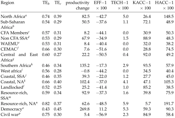
Table 2: Efficiency scores and percentage change of quadripartite decomposition indexes, 1970−2007.
Region TEb TEc productivity EFF−1 TECH−1 KACC−1 HACC−1
change × 100 × 100 × 100 × 100 North Africaa 0.74 0.39 82.5 −42.7 5.0 26.4 148.5 Sub-Saharan Africab 0.54 0.29 50.5 −37.6 1.1 72.1 48.9 CFA Membersc 0.57 0.31 8.2 −44.1 0.0 30.9 50.3
Non CFA SSAd 0.53 0.29 67.9 −34.9 1.5 88.9 48.3
WAEMUe 0.53 0.31 8.4
−40.4 0.0 32.0 38.2
CEMACf 0.66 0.30 7.6
−51.6 0.0 28.8 74.5
Central and East Africag 0.60 0.27 22.2 −50.5 0.4 92.0 49.2 Southern Africah 0.46 0.34 135.2 −17.3 2.9 93.5 57.9 West africai 0.56 0.28 −0.8 −44.2 0.0 34.5 40.4 Coastal, SSAj 0.46 0.35 39.3 −22.0 1.2 27.7 45.0 Coastal, NAk 0.66 0.40 102.4 −37.0 4.1 47.1 105.3 Landlockedl 0.52 0.25 25.2 −41.4 1.0 85.2 38.5 Resource-rich, SSAm 0.59 0.34 92.9 −37.3 1.6 39.8 75.9 Resource-rich, NAn 0.82 0.37 62.6 −48.5 5.9 5.7 191.7 Democracyo 0.43 0.45 269.8 11.2 5.3 59.3 90.3 Civil warp 0.75 0.30 5.4 −56.9 2.3 84.9 58.4
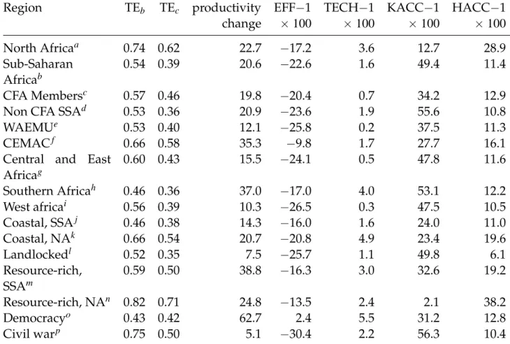
a: Algeria, Egypt, Morocco, Tunisia;b: Benin, Botswana, Burundi, Cameroon, Central
Malawi, Mali, Mauritania, Mauritius, Mozambique, Namibia, Niger, Rwanda, Senegal, Sierra Leone, South Africa, Sudan, Swaziland, Tanzania, Togo, Uganda, Zambia, Zim-babwe;c: Benin, Cameroon, Central African Republic, Cote d’Ivoire, Gabon, Mali, Niger,
Senegal, Togo; d: Botswana, Burundi, Congo, Gambia, Ghana, Kenya, Lesotho, Liberia,
Malawi, Mauritania, Mauritius, Mozambique, Namibia, Rwanda, Sierra Leone, South Africa, Sudan, Swaziland, Tanzania, Uganda, Zambia, Zimbabwe;e: Benin, Cote d’Ivoire, Mali, Niger, Senegal, Togo; f: Cameroon, Central African Republic, Gabon; g: Burundi, Cameroon, Central African Republic, Congo, Gabon, Kenya, Rwanda, Sudan, Tanzania, Uganda;h: Botswana, Lesotho, Malawi, Mauritius, Mozambique, Namibia, South Africa, Swaziland, Zambia, Zimbabwe; i: Benin, Cote d’Ivoire, Gambia, Ghana, Liberia, Mali, Mauritania, Niger, Senegal, Sierra Leone, Togo; j: Benin, Cote d’Ivoire, Ghana, Kenya, Mauritius, Mozambique, Senegal, South Africa, Tanzania, Togo; k: Egypt, Morocco; l:
Burundi, Central African Republic, Malawi, Mali, Niger, Sudan, Uganda, Zimbabwe; m: Botswana, Cameroon, Congo, Gabon, Namibia, Sierra Leone, Zambia;n: Algeria, Tunisia;
o: Botswana, Mauritius, Namibia; p: Algeria, Burundi, Liberia, Morocco, Mozambique,
Appendix
1
Comparison 1970–1979
Capital per efficiency unit of labor
20200 746760 1473320 2199880 2926440 3653000 600 2940 5280 7620 9960 12300
Output per efficiency unit of labor
DZA BENBWA BDI CMR CAF COG CIVEGY GAB GMB GHA KEN LSO LBR MWI MLI MRT MUS MAR MOZ NAM NER RWA SEN SLE ZAF SDN SWZ TZA TGO TUN UGA ZMB ZWE DZA BEN BWA BDI CMR CAF COG CIV EGY GAB GMB GHA KEN LSO LBR MWI MLI MRT MUS MAR MOZ NAM NER RWA SEN SLE ZAF SDN SWZ TZA TGO TUN UGA ZMB ZWE Production Frontier in 1970 Production Frontier in 1979
Figure 4: Production frontiers in 1970 and 1979
Notes: The bold italic abbreviations show the 1970 observations and the normal font abbreviations show the
1979 observations. The solid line represents the 1970 production frontier and then dotted line presents the 1979 production frontier.
0
.5
1
1.5
2
Kernel estimated density
0.2 0.4 0.6 0.8 1.0
Efficiency Index
1970 Distribution 1979 Distribution
Figure 5: Distributions of efficiency index in 1970 and 1979.
Notes: The solid vertical line represents mean of 1970 efficiency distribution and the the dashed curve is the
3.5e−07
6.1e−05
1.2e−04
1.8e−04
Kernel estimated density
0 5000 10000 15000 20000 25000 30000
Output per Worker
y1970 y1970 * KACC y1979
(a) Effect of Capital Deepening
3.5e−07
6.1e−05
1.2e−04
1.8e−04
Kernel estimated density
0 5000 10000 15000 20000 25000 30000
Output per Worker
y1970
y1970 * KACC * HACC y1979
(b) Effect of Human Capital Accumulation
3.5e−07
6.1e−05
1.2e−04
1.8e−04
Kernel estimated density
0 5000 10000 15000 20000 25000 30000
Output per Worker
y1970
y1970 * KACC * HACC * EFF y1979
(c) Effect of Efficiency Change
Figure 6: Counterfactual Distributions of Output per Worker. Sequence of introducing effects of decomposition: KACC, HACC, and EFF
Notes: In each panel, the solid curve is the actual 1970 distribution and the dashed curve is the actual 1979
distribution. The dotted curves in each panel are the counterfactual distributions isolating, sequentially, the effects of capital deepening, human capital accumulation, and efficiency change on the 1970 distribution.
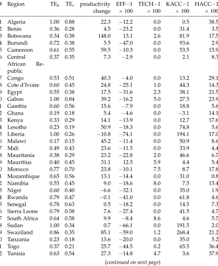
Table 3: Efficiency scores and percentage change of quadripartite decomposition indexes, 1970−1979.
# Region TEb TEc productivity EFF−1 TECH−1 KACC−1 HACC−1
change × 100 × 100 × 100 × 100 1 Algeria 1.00 0.88 22.3 −12.2 0.0 0.5 38.5 2 Benin 0.36 0.28 4.5 −23.2 0.0 31.4 3.5 3 Botswana 0.34 0.38 148.0 13.1 2.6 81.9 17.5 4 Burundi 0.72 0.38 5.5 −47.0 0.0 93.6 2.9 5 Cameroon 0.61 0.55 59.5 −10.3 0.0 53.5 15.9 6 Central African Re-public 0.37 0.35 7.3 −2.9 0.0 2.1 8.3 7 Congo 0.53 0.51 40.3 −4.0 0.0 13.2 29.1 8 Cote d’Ivoire 0.60 0.45 24.8 −25.1 1.0 44.3 14.3 9 Egypt 0.55 0.38 17.5 −31.6 2.3 38.1 21.5 10 Gabon 1.00 0.84 39.2 −16.2 5.0 27.5 23.9 11 Gambia 0.60 0.56 15.6 −7.9 0.0 18.8 5.6 12 Ghana 0.19 0.18 5.4 −4.6 0.0 −3.1 14.1 13 Kenya 0.33 0.29 14.1 −13.9 0.0 12.7 17.6 14 Lesotho 0.23 0.19 50.9 −18.3 0.0 74.8 5.6 15 Liberia 1.00 0.26 −10.8 −74.1 0.0 194.1 17.0 16 Malawi 0.17 0.15 45.2 −11.4 0.0 50.9 8.6 17 Mali 0.49 0.43 23.6 −11.5 0.0 33.9 4.4 18 Mauritania 0.38 0.29 23.2 −22.8 2.0 46.6 6.7 19 Mauritius 0.40 0.45 31.1 12.5 5.9 4.4 5.4 20 Morocco 0.77 0.70 23.8 −10.1 7.5 8.7 17.8 21 Mozambique 0.65 0.56 13.1 −14.4 0.0 31.0 0.8 22 Namibia 0.55 0.45 9.0 −18.6 8.0 7.5 15.4 23 Niger 0.60 0.40 −6.6 −32.1 0.0 35.0 1.9 24 Rwanda 0.79 0.47 −0.1 −41.0 0.0 61.8 4.6 25 Senegal 0.78 0.63 0.5 −18.2 0.0 14.5 7.3 26 Sierra Leone 0.79 0.58 7.6 −27.4 0.0 41.5 4.7 27 South Africa 0.64 0.58 9.9 −8.4 8.6 4.6 5.7 28 Sudan 1.00 0.34 0.7 −66.1 0.0 191.5 2.0 29 Swaziland 0.86 0.35 85.1 −59.0 1.2 268.4 21.2 30 Tanzania 0.23 0.18 13.6 −20.0 0.0 35.0 5.2 31 Togo 0.37 0.21 25.7 −44.5 0.2 65.5 36.4 32 Tunisia 0.63 0.54 27.3 −14.8 4.7 3.6 37.9
Table 3 (Continued)
# Region TEb TEc productivity EFF−1 TECH−1 KACC−1 HACC−1
change × 100 × 100 × 100 × 100 33 Uganda 0.46 0.37 −24.7 −19.2 0.0 −12.7 6.7 34 Zambia 0.33 0.16 −31.8 −50.7 5.1 3.0 27.7 35 Zimbabwe 0.41 0.35 9.3 −15.1 8.6 4.2 13.7 average 0.56 0.42 20.8 −22.0 1.8 45.2 13.4 weighted aver-age 0.59 0.44 13.9 −22.2 2.2 35.2 13.8
Table 4: Efficiency scores and percentage change of quadripartite decomposition indexes, 1970−1979.
Region TEb TEc productivity EFF−1 TECH−1 KACC−1 HACC−1
change × 100 × 100 × 100 × 100 North Africaa 0.74 0.62 22.7 −17.2 3.6 12.7 28.9 Sub-Saharan Africab 0.54 0.39 20.6 −22.6 1.6 49.4 11.4 CFA Membersc 0.57 0.46 19.8 −20.4 0.7 34.2 12.9
Non CFA SSAd 0.53 0.36 20.9 −23.6 1.9 55.6 10.8
WAEMUe 0.53 0.40 12.1
−25.8 0.2 37.5 11.3
CEMACf 0.66 0.58 35.3
−9.8 1.7 27.7 16.1
Central and East Africag 0.60 0.43 15.5 −24.1 0.5 47.8 11.6 Southern Africah 0.46 0.36 37.0 −17.0 4.0 53.1 12.2 West africai 0.56 0.39 10.3 −26.5 0.3 47.5 10.5 Coastal, SSAj 0.46 0.38 14.3 −16.0 1.6 24.0 11.0 Coastal, NAk 0.66 0.54 20.7 −20.8 4.9 23.4 19.6 Landlockedl 0.52 0.35 7.5 −25.7 1.1 49.8 6.1 Resource-rich, SSAm 0.59 0.50 38.8 −16.3 3.0 32.6 19.2 Resource-rich, NAn 0.82 0.71 24.8 −13.5 2.4 2.1 38.2 Democracyo 0.43 0.42 62.7 2.4 5.5 31.2 12.8 Civil warp 0.75 0.50 5.1 −30.4 2.2 56.3 10.4
a: Algeria, Egypt, Morocco, Tunisia;b: Benin, Botswana, Burundi, Cameroon, Central
Malawi, Mali, Mauritania, Mauritius, Mozambique, Namibia, Niger, Rwanda, Senegal, Sierra Leone, South Africa, Sudan, Swaziland, Tanzania, Togo, Uganda, Zambia, Zim-babwe;c: Benin, Cameroon, Central African Republic, Cote d’Ivoire, Gabon, Mali, Niger,
Senegal, Togo; d: Botswana, Burundi, Congo, Gambia, Ghana, Kenya, Lesotho, Liberia,
Malawi, Mauritania, Mauritius, Mozambique, Namibia, Rwanda, Sierra Leone, South Africa, Sudan, Swaziland, Tanzania, Uganda, Zambia, Zimbabwe;e: Benin, Cote d’Ivoire, Mali, Niger, Senegal, Togo; f: Cameroon, Central African Republic, Gabon; g: Burundi, Cameroon, Central African Republic, Congo, Gabon, Kenya, Rwanda, Sudan, Tanzania, Uganda;h: Botswana, Lesotho, Malawi, Mauritius, Mozambique, Namibia, South Africa, Swaziland, Zambia, Zimbabwe; i: Benin, Cote d’Ivoire, Gambia, Ghana, Liberia, Mali, Mauritania, Niger, Senegal, Sierra Leone, Togo; j: Benin, Cote d’Ivoire, Ghana, Kenya, Mauritius, Mozambique, Senegal, South Africa, Tanzania, Togo; k: Egypt, Morocco; l:
Burundi, Central African Republic, Malawi, Mali, Niger, Sudan, Uganda, Zimbabwe; m: Botswana, Cameroon, Congo, Gabon, Namibia, Sierra Leone, Zambia;n: Algeria, Tunisia;
o: Botswana, Mauritius, Namibia; p: Algeria, Burundi, Liberia, Morocco, Mozambique,
2
Comparison 1980–1989
Capital per efficiency unit of labor
23100 761600 1500100 2238600 2977100 3715600 300 2700 5100 7500 9900 12300
Output per efficiency unit of labor
DZA BEN BWA BDI CMR CAF COG CIVEGY GAB GMB GHA KEN LSO LBR MWI MLI MRT MUS MAR MOZ NAM NER RWA SEN SLE ZAF SDN SWZ TZA TGO TUN UGA ZMB ZWE DZA BEN BWA BDI CMR CAF COG CIV EGY GAB GMB GHA KEN LSO LBR MWI MLI MRT MUS MAR MOZ NAM NER RWA SEN SLE ZAF SDN SWZ TZA TGO TUN UGAZMB ZWE Production Frontier in 1980 Production Frontier in 1989
Figure 7: Production frontiers in 1980 and 1989
Notes: The bold italic abbreviations show the 1980 observations and the normal font abbreviations show the
1989 observations. The solid line represents the 1980 production frontier and then dotted line presents the 1989 production frontier.
0 .5 1 1.5 2 2.5
Kernel estimated density
0.2 0.4 0.6 0.8
Efficiency Index
1980 Distribution 1989 Distribution
Figure 8: Distributions of efficiency index in 1980 and 1989.
Notes: The solid vertical line represents mean of 1980 efficiency distribution and the the dashed curve is the