HAL Id: hal-02302740
https://hal.telecom-paris.fr/hal-02302740
Submitted on 1 Oct 2019
HAL is a multi-disciplinary open access
archive for the deposit and dissemination of
sci-entific research documents, whether they are
pub-lished or not. The documents may come from
teaching and research institutions in France or
abroad, or from public or private research centers.
L’archive ouverte pluridisciplinaire HAL, est
destinée au dépôt et à la diffusion de documents
scientifiques de niveau recherche, publiés ou non,
émanant des établissements d’enseignement et de
recherche français ou étrangers, des laboratoires
publics ou privés.
Knowledge Representation and Rule Mining in
Entity-Centric Knowledge Bases
Fabian Suchanek, Jonathan Lajus, Armand Boschin, Gerhard Weikum
To cite this version:
Fabian Suchanek, Jonathan Lajus, Armand Boschin, Gerhard Weikum. Knowledge Representation
and Rule Mining in Entity-Centric Knowledge Bases. Doctoral. Italy. 2019. �hal-02302740�
Knowledge Representation and Rule Mining
in Entity-Centric Knowledge Bases
Fabian M. Suchanek1, Jonathan Lajus1, Armand Boschin1, and Gerhard
Weikum2
1 Telecom Paris, Institut Polytechnique de Paris 2
Max Planck Institute for Informatics
Abstract. Entity-centric knowledge bases are large collections of facts about entities of public interest, such as countries, politicians, or movies. They find applications in search engines, chatbots, and semantic data mining systems. In this paper, we first discuss the knowledge represen-tation that has emerged as a pragmatic consensus in the research com-munity of entity-centric knowledge bases. Then, we describe how these knowledge bases can be mined for logical rules. Finally, we discuss how entities can be represented alternatively as vectors in a vector space, by help of neural networks.
1
Introduction
1.1 Knowledge Bases
When we send a query to Google or Bing, we obtain a set of Web pages. However, in some cases, we also get more information. For example, when we ask “When was Steve Jobs born?”, the search engine replies directly with “February 24, 1955”. When we ask just for “Steve Jobs”, we obtain a short biography, his birth date, quotes, and spouse. All of this is possible because the search engine has a huge repository of knowledge about people of common interest. This knowledge takes the form of a knowledge base (KB).
The KBs used in such search engines are entity-centric: they know indi-vidual entities (such as Steve Jobs, the United States, the Kilimanjaro, or the Max Planck Society), their semantic classes (such as SteveJobs is-a computer-Pioneer, SteveJobs is-a entrepreneur ), relationships between entities (e.g., Steve-Jobs founded AppleInc, SteveSteve-Jobs hasInvented iPhone, SteveSteve-Jobs hasWonPrize NationalMedalOfTechnology, etc.) as well as their validity times (e.g., SteveJobs wasCEOof Pixar [1986,2006] ).
The idea of such KBs is not new. It goes back to seminal work in Artificial Intelligence on universal knowledge bases in the 1980s and 1990s, most notably, the Cyc project [41] at MCC in Austin and the WordNet project [19] at Princeton University. These knowledge collections were hand-crafted and manually curated. In the last ten years, in contrast, KBs are often built automatically by extracting information from the Web or from text documents. Salient projects with publicly available resources include KnowItAll (UW Seattle, [17]), ConceptNet (MIT,
[44]), DBpedia (FU Berlin, U Mannheim, & U Leipzig, [40]), NELL (CMU, [9]), BabelNet (La Sapienza, [58]), Wikidata (Wikimedia Foundation, [77]), and YAGO (Telecom Paris & Max Planck Institute, [70]). Commercial interest in KBs has been strongly growing, with projects such as the Google Knowledge Graph [15] (including Freebase [6]), Microsoft’s Satori, Amazon’s Evi, LinkedIn’s Knowledge Graph, and the IBM Watson KB [20]. These KBs contain many millions of entities, organized in hundreds to hundred thousands of semantic classes, and hundred millions of relational facts between entities. Many public KBs are interlinked, forming the Web of Linked Open Data [5].
1.2 Applications
KBs are used in several applications, including the following:
Semantic Search and Question Answering. Both the Google search en-gine [15] and Microsoft Bing3use KBs to give intelligent answers to queries, as we have seen above. They can answer simple factual questions, provide movie showtimes, or show a list of “best things to do” at a travel destination. Wolfram Alpha4is another prominent example of a question answering system. The IBM Watson system [20] used knowledge from a KB to win against human champions in the TV quiz show Jeopardy.
Intelligent Assistants. Chatbots such as Apple’s Siri, Amazon’s Alexa, Google’s Allo, or Microsoft’s Cortana aim to help a user achieve daily tasks. The bots can, e.g., suggest restaurants nearby, answer simple factual questions, or manage calendar events. The background knowledge that the bots need for this work usually comes from a KB. With embodiments such as Amazon’s Echo system or Google Home, such assistants will share more and more people’s homes in the future. Other companies, too, are experimenting with chat bots that treat customer requests or provide help to users.
Semantic Data Mining. Daily news, social media, scholarly publications, and other Web contents are the raw inputs for analytics to obtain insights on busi-ness, politics, health, and more. KBs can help to discover and track entities and relationships in order to generate opinion maps, informative recommendations, and other kinds of intelligence towards decision making. For example, we can mine the gender bias from newspapers, because the KB knows the gender of people (see [71] for a survey). There is an entire domain of research dedicated to “predictive analytics”, i.e., the prediction of events based on past events.
1.3 Knowledge Representation and Rule Mining
In this article, we first discuss how the knowledge is usually represented in entity-centric KBs. The field of knowledge representation has a long history,
3
http://blogs.bing.com/search/2013/03/21/understand-your-world-with-bing/
4
and goes back to the early days of Artificial Intelligence. It has developed nu-merous knowledge representation models, from frames and KL-ONE to recent variants of description logics. The reader is referred to survey works for com-prehensive overviews of historical and classical models [62,67]. In this article, we discuss the knowledge representation that has emerged as a pragmatic consensus in the research community of entity-centric knowledge bases.
In the second part of this article, we discuss logical rules on knowledge bases. A logical rule can tell us, e.g., that if two people are married, then they (usually) live in the same city. Such rules can be mined automatically from the knowledge base, and they can serve to correct the data or fill in missing information. We discuss first classical Inductive Logic Programming approaches, and then show how these can be applied to the case of knowledge bases.
In the third part of this article, we discuss an alternative way to represent entities: as vectors in a vector space. Such so-called embeddings can be learned by neural networks from a knowledge base. The embeddings can then help deduce new facts – much like logical rules.
2
Knowledge Representation
2.1 Entities
2.1.1 Entities of Interest
The most basic element of a KB is an entity. An entity is any abstract or concrete object of fiction or reality, or, as Bertrand Russell puts it in his Principles of Mathematics [81]:
Definition 1 (Entity): An entity is whatever may be an object of thought. This definition is completely all-embracing. Steve Jobs, the Declaration of Independence of the United States, the Theory of Relativity, and a molecule of water are all entities. Events (such as the French Revolution), are entities, too. An entity does not even have to exist: Harry Potter, e.g., is a fictional entity. Phlogiston was presumed to be the substance that makes up heat. It turned out to not exist – but it is still an entity.
KBs model a part of reality. This means that they choose certain entities of interest, give them names, and put them into a structure. Thus, a KB is a structured view on a selected part of the world. KBs typically model only distinct entities. This cuts out a large portion of the world that consists of variations, flows and transitions between entities. Drops of rain, for instance, fall down, join in a puddle and may be splattered by a passing car to form new drops [66]. KBs will typically not model these phenomena. This choice to model only discrete entities is a projection of reality; it is a grid through which we see only distinct things. Many entities consist of several different entities. A car, for example, consists of wheels, a bodywork, an engine, and many other pieces. The engine consists of the pistons, the valves, and the spark plug. The valves consist again of several parts, and so on, until we ultimately arrive at the level of atoms or
below. Each of these components is an entity. However, KBs will typically not be concerned with the lower levels of granularity. A KB might model a car, possibly its engine and its wheels, but most likely not its atoms. In all of the following, we will only be concerned with the entities that a KB models.
Entities in the real world can change gradually. For example, the Greek philosopher Eubilides asks: If one takes away one molecule of an object, will there still be the same object? If it is still the same object, this invites one to take away more molecules until the object disappears. If it is another object, this forces one to accept that two distinct objects occupy the same spatio-temporal location: The whole and the whole without the molecule. A related problem is the question of identity. The ancient philosopher Theseus uses the example of a ship: Its old planks are constantly being substituted. One day, the whole ship has been replaced and Theseus asks, “Is it still the same ship?”. To cope with these problems, KBs typically model only atomic entities. In a KB, entities can only be created and destroyed as wholes.
2.1.2 Identifiers and Labels
In computer systems (as well as in writing of any form), we refer to entities by identifiers.
Definition 2 (Identifier): An identifier for an entity is a string of characters that represents the entity in a computer system.
Typically, these identifiers take a human-readable form, such as ElvisPresley for the singer Elvis Presley. However, some KBs use abstract identifiers. Wiki-data, e.g., refers to Elvis Presley by the identifier Q303, and Freebase by /m/02jq1. This choice was made so as to be language-independent, and so as to provide an identifier that is stable in time. If, e.g., Elvis Presley reincarnates in the future, then Q303 will always refer to the original Elvis Presley. It is typically assumed that there exists exactly one identifier per entity in a KB. For what follows, we will not distinguish identifiers from entities, and just talk of entities instead.
Entities have names. For example, the city of New York can be called “city of New York”, “Big Apple”, or “Nueva York”. As we see, one entity can have several names. Vice versa, the same name can refer to several entities. “Paris”, e.g., can refer to the city in France, to a city of that name in Texas, or to a hero of Greek mythology. Hence, we need to carefully distinguish names – single words or entire phrases – from their senses – the entities that they denote. This is done by using labels.
Definition 3 (Label): A label for an entity is a human-readable string that names the entity.
If an entity has several labels, the labels are called synonymous. If the same label refers to several entities, the label is polysemous. Not all entities have labels. For example, your kitchen chair is clearly an entity, but it probably does not have any particular label. An entity that has a label is called a named entity.
KBs typically model mainly named entities. There is one other type of entities that appears in KBs: literals.
Definition 4 (Literal): A literal is a fixed value that takes the form of a string of characters.
Literals can be pieces of text, but also numbers, quantities, or timestamps. For example, the label “Big Apple” for the city of New York is a literal, as is the number of its inhabitants (8,175,133).
2.2 Classes
2.2.1 Classes and Instances
KBs model entities of the world. They usually group entities together to form a class:
Definition 5 (Class): A class (also: concept, type) is a named set of entities that share a common trait. An element of that set is called an instance of the class.
Under this definition, the following are classes: The class of singers (i.e., the set of all people who sing professionally), the class of historical events in Latin America, and the class of cities in Germany. Some instances of these classes are, respectively, Elvis Presley, the independence of Argentina, and Berlin. Since everything is an entity, a class is also an entity. It has (by definition) an identifier and a label.
Theoretically, KBs can form classes based on arbitrary traits. We can, e.g., construct the class of singers whose concerts were the first to be broadcast by satellite. This class has only one instance (Elvis Presley). We can also construct the class of left-handed guitar players of Scottish origin, or of pieces of music that the Queen of England likes. There are several theories as to whether humans actually build and use classes, too [46]. Points of discussion are whether humans form crisp concepts, and whether all elements of a concept have the same degree of membership. For the purpose of KBs, however, classes are just sets of entities. It is not always easy to decide whether something should be modeled as an instance or as a class. We could construct, e.g., for every instance a singleton class that contains just this instance (e.g., the class of all Elvis Presleys). Some things of the world can be modeled both as instances and as classes. A typical example is iPhone. If we want to designate the type of smartphone, we can model it as an instance of the class of smartphone brands. However, if we are interested in the iPhones owned by different people and want to capture them individually, then iPhone should be modeled as a class. A similar observation holds for abstract entities such as love. Love can be modeled as an instance of the class emotion, where it resides together with the emotions of anger, fear, and joy. However, when we want to model individual feelings of love, then love would be a class. Its instances are the different feelings of love that different people have. It is our choice how we wish to model reality.
A pragmatic test of whether something should be modeled as a class is as follows: If we are interested in the plural form of a word or phrase, then we should model it as a class. If we talk, e.g., about “iPhones”, then we model several instances of iPhones, and hence iPhone should be a class. If we only talk about “iPhone” along with other brand names (such as “HTC One”), then iPhone may well be considered an instance. Analogously, if we talk of “love” only in singular, then we may model it as an instance, along with other emotions. If we talk of “loves” (as in “Elvis had many loves during his time as a star”), then love is the set of all love affairs – and thus a class. The reason for this test is that only countable nouns can be classes, and only countable nouns can be put into plural. Another method to distinguish classes from instances is to say “An X”, or “Every X”. If that is possible, then X is best modeled as a class, because it can have instances. For example, it is possible to say “a CEO”, but not “a Steve Jobs”. Hence, ceo should be a class, and SteveJobs should not. If we can say “This is X”, then X is an instance – as in “This is Steve Jobs”. If we can say “X is a Y”, then X is an instance of Y – as in “Steve Jobs is a CEO”.
A particular case are mass nouns like “milk”. The word “milk” (in the sense of the liquid) does not have a plural form. Therefore, we could model it as an instance (e.g., as an instance of the class of liquids). However, if we are interested in individual servings of milk, such as bottles of milk, then we can model it as a class, servingOfMilk.
Some KBs do not make the distinction between classes and instances (e.g., the SKOS vocabulary, [84]). In these KBs, everything is an entity. There is, however, usually a “is more general than” link between a more special entity and a more general entity. Such a KB may contain, e.g., the knowledge that iPhone is more special than smartphone, without worrying whether one of them is a class. The distinction between classes and instances adds a layer of granularity. This granularity is used, e.g., to define the domains and ranges of relations, as we shall see in Section 2.3.
2.2.2 Taxonomies
Definition 6 (Subsumption): Class A is a subclass of class B if A is a subset of B.
For example, the class of singers is a subclass of the class of persons, because every singer is a person. We also say that the class of singers is a specialization of the class of persons, or that singer is subsumed by or included in person. Vice versa, we say that person is a superclass or a generalization of the class of singers. Technically speaking, two equivalent classes are subclasses of each other. This is the way the RDFS standard models subclasses [83]. We say that a class is a proper subclass of another class, if the second contains more entities than the first. We use the notion of subclass here to refer to proper subclasses only.
It is important not to confuse class inclusion with the relationship between parts and wholes. For example, an arm is a part of the human body. That does not mean, however, that every arm is a human body. Hence, arm is not a subclass
of body. In a similar manner, New York is a part of the US. That does not mean that New York would be a subclass of the US. Neither New York nor the US are classes, so they cannot be subclasses of each other.
Class inclusion is transitive: If A is a subclass of B, and B is a subclass of C, then A is a subclass of C. For example, viper is a subclass of snake, and snake is a subclass of reptile. Hence, by transitivity, viper is also a subclass of reptile. We say that a class is a direct subclass of another class, if there is no class in the KB that is a superclass of the former and a subclass of the latter. When we talk about subclasses, we usually mean only direct subclasses. The other subclasses are transitive subclasses. Since classes can be included in other classes, they can form an inclusion hierarchy – a taxonomy.
Definition 7 (Taxonomy): A taxonomy is a directed graph, where the nodes are classes and there is an edge from class X to class Y if X is a proper direct subclass of Y.
The notion of taxonomy is known from biology. Zoological or botanic species form a taxonomy: tiger is a subclass of cat. cat is a subclass of mammal, and so on. This principle carries over to all other types of classes. We say, e.g., that internetCompany is a subclass of company, and that company is a subclass of organization, etc. Since a taxonomy models proper inclusion, it follows that the taxonomic graph is acyclic: If a class is the subclass of another class, then the latter cannot be a subclass of the former. Thus, a taxonomy is a directed acyclic graph. A taxonomy does not show the transitive subclass edges. If the graph contains transitive edges, we can always remove them. Given a finite directed acyclic graph with transitive edges, the set of direct edges is unique [2].
Transitivity is often essential in applications. For example, consider a question-answering system where a user asks for artists that are married to actors. If the KB only knew about Elvis Presley and Priscilla Presley being in the classes rockSinger and americanActress, the question could not be answered. However, by reasoning that rockSingers are also singers, who in turn are artists and americanActresses being actresses, it becomes possible to give this correct answer.
Usually (but not necessarily), taxonomies are connected graphs: Every node in the graph is, directly or indirectly, linked to every other node. Usually, the taxonomies have a single root, i.e., a single node that has no outgoing edges. This node identifies the most general class, of which every other class is a subclass. In zoological KBs, this may be class animal. In a person database, it may be the class person. In a general-purpose KB, this class has to be the most general possible class. In YAGO and Wordnet, the class is entity. In the RDF standard, it is called resource [82]. In the OWL standard [85], the highest class that does not include literals is called thing.
Some taxonomies have at most one outgoing edge per node. Then, the tax-onomy forms a tree. The biological taxtax-onomy, e.g., forms a tree, as does the Java class hierarchy. However, there can be taxonomies where a class has two distinct direct superclasses. For example, if we have the class singer and the classes of woman and man, then the class femaleSinger has two superclasses: singer and
woman. Note that it would be wrong to make singer a subclass of man and woman (as if to say that singers can be men or women). This would actually mean that all singers are at the same time men and women.
When a taxonomy includes a “combination class” such as FrenchFe-maleSingers, then this class can have several superclasses. FrenchFeFrenchFe-maleSingers, e.g., can have as direct superclasses FrenchPeople, Women, and Singers. In a similar manner, one entity can be an instance of several classes. Albert Einstein, e.g., is an instance of the classes physicist, vegetarian, and violinPlayer.
When we populate a KB with new instances, we usually try to assign them to the most specific suitable class. For example, when we want to place Bob Dylan in our taxonomy, we would put him in the class americanBluesSinger, if we have such a class, instead of in the class person. However, if we lack more specific information about the instance, then we might be forced to put it into a general class. Some named entity recognizers, e.g., distinguish only between organizations, locations, and people, which means that it is hard to populate more specific classes. It may also happen that our taxonomy is not specific enough at the leaf level. For example, we may encounter a musician who plays the Arabic oud, but our taxonomy does not have any class like oudPlayer. Therefore, a class may contain more instances than the union of its subclasses. That is, for a class C with subclasses C1, . . . , Ck, the invariant is ∪i=1..kCk ⊆ C, but
∪i=1..kCk= C is often false.
2.2.3 Special Cases
Some KBs assign literals to classes, too. For example, the literal “Hello” can be modeled as an instance of the class string. Such literal classes can also form taxonomies. For example, the class nonNegativeIntegers is a subclass of the class of integers, which is again a subclass of the more general class numbers.
We already observed that classes are entities. Thus, we can construct classes that contain other classes as instances. For example, we can construct the class of all classes class ={car, person, scientist, ...}. This leads to awkward questions about self-containment, reminiscent of Bertrand Russel’s famous set of sets that do not include themselves. The way this is usually solved [82] is to distinguish the class (as an abstract concept) from the extension of the class (the set of its instances). For example, the class of singers is the abstract concept of people who sing. Its extension is the set {Elvis, Madonna, ...}. In this way, a class is not a set, but just an abstract entity. Therefore, the extension of a class can contain another class. This is, however, a rather theoretical problem, and in what follows, we will not distinguish classes from their extensions.
To distinguish classes from other entities, we call an entity that is neither a class nor a literal an instance or a common entity.
2.3 Relations
2.3.1 Relations and Statements
KBs model also relationships between entities:
Definition 8 (Relation): A relationship (also: relation) over the classes C1, ..., Cn is a named subset of the Cartesian product C1× ... × Cn.
For example, if we have the classes person, city, and year, we may construct the birth relationship as a subset of the cartesian product person×city×year. It will contain tuples of a person, their city of birth, and their year of birth. For example, hElvisP resley, T upelo, 1935i ∈ birth. In a similar manner, we can construct tradeAgreement as a subset of country×country×commodity. This relation can contain tuples of countries that made a trade agreement concerning a commodity. Such relationships correspond to classical relations in algebra or databases.
As always in matters of knowledge representation (or, indeed, informatics in general), the identifier of a relationship is completely arbitrary. We could, e.g., call the birth relationship k42, or, for that matter, death. Nothing hinders us to populate the birth relationship with tuples of a person, and the time and place where that person ate an ice cream. However, most KBs aim to model reality, and thus use identifiers and tuples that correspond to real-world relationships.
If hx1, ..., xni ∈ R for a relationship R, we also write R(x1, ..., xn). In the
example, we write birth(ElvisP resley, T upelo, 1935). The classes of R are called the domains of R. The number of classes n is called the arity of R. hx1, ..., xni
is a tuple of R. R(x1, ..., xn) is called a statement, fact, or record. The elements
x1, ..., xn are called the arguments of the facts. Finally, a knowledge base, in its
simplest form, is a set of statements. For example, a KB can contain the relations birth, death and marriage, and thus model some of the aspects of people’s lives.
2.3.2 Binary Relations
Definition 9 (Binary Relation): A binary relation is a relation of arity 2. Examples of binary relations are birthPlace, friendOf, or marriedTo. The first argument of a binary fact is called the subject, and the second argument is called the object of the fact. The relationships are sometimes called properties. Relationships that have literals as objects, and that have at most one object per subject are sometimes called attributes. Examples are hasBirthDate or hasISBN. The domain of a binary relation R ⊂ A × B is A, i.e., the class from which the subjects are taken. B is called the range of R. For example, the domain of birth-Place is person, and its range is city. The inverse of a binary relation R is a relation R−1, such that R−1(x, y) iff R(x, y). For example, the inverse relation of hasNationality (between a person and a country) is hasNationality−(between a country and a person) – which we could also call hasCitizen.
Any n-ary relation R with n > 2 can be split into n binary relations. This works as follows. Assume that there is one argument position i that is a key,
i.e., every fact R(x1, ..., xn) has a different value for xi. In the previously
in-troduced 3-ary birth relationship, which contains the person, the birth place, and the birth date, the person is the key: every person is born only once at one place. Without loss of generality, let the key be at position i = 1. We introduce binary relationships R2, ..., Rn. In the example, we introduce
birth-Place for the relation between the person and the birth place, and birthDate for the relation between the person and the birth year. Every fact R(x1, ..., xn)
gets rewritten as R2(x1, x2), R3(x1, x3), R4(x1, x4), ..., Rn(x1, xn). In the
exam-ple, the fact birth(Elvis,Tupelo,1935) gets rewritten as birthPlace(Elvis,Tupelo) and birthDate(Elvis,1935). Now assume that a relation R has no key. As an exam-ple, consider again the tradeAgreement relationship. Obviously, there is no key in this relationship, because any country can make any number of trade-agreements on any commodity. We introduce binary relationships R1, ...Rn for every
argu-ment position of R. For tradeAgreeargu-ment, these could be country1, country2 and tradeCommodity. For each fact of R, we introduce a new entity, an event entity. For example, if the US and Brazil make a agreement on coffee, trade-Agreement(Brazil,US,Coffee), then we create coffeeAgrBrUs. This entity repre-sents the fact that these two countries made this agreement. In general, every fact R(x1, ..., xn) gives rise to an event entity ex1,...,xn. Then, every fact R(x1, ..., xn)
is rewritten as R1(ex1,...,xn, x1), R2(ex1,...,xn, x2), ..., Rn(ex1,...,xn, xn). In the
ex-ample, country1(coffeeAgrBrUs, Brazil), country2(coffeeAgrBrUs, US), trade-Commodity(coffeeAgrBrUs, Coffee). This way, any n-ary relationship with n > 2 can be represented as binary relationships. For n = 1, we can always invent a binary relation hasProperty, and use the relation as an additional argument. For example, instead of male(Elvis), we can say hasProperty(Elvis, male).
The advantage of binary relationships is that they can express facts even if one of the arguments is missing. If, e.g., we know only the birth year of Steve Jobs, but not his birth place, then we cannot make a fact with the 3-ary relation birth ⊂ person×city×year. We have to fill the missing arguments, e.g., with null values. If the relationship has a large arity, many of its arguments may have to be null values. In the case of binary relationships, in contrast, we can easily state birthDate(SteveJobs, 1955), and omit the birthPlace fact. Another disadvantage of n-ary relationships is that they do not allow adding new pieces of information a posteriori. If, e.g., we forgot to declare the astrological ascendant as an argument to the 3-ary relation birth, then we cannot add the ascendant for Steve Job’s birth without modifying the relationship. In the binary world, in contrast, we can always add a new relationship birthAscendant. Thus, binary relationships offer more flexibility. This flexibility can be a disadvantage, because it allows adding incomplete information (e.g., a birth place without a birth date). However, since knowledge bases are often inherently incomplete, binary relationships are usually the method of choice.
2.3.3 Functions
Definition 10 (Function): A function is a binary relation that has for each subject at most one object.
Typical examples for functions are birthPlace and hasLength: Every person has at most one birth place and every river has at most one length. The relation ownsCar, in contrast, is not a function, because a (rich) person can own multiple cars. In our terminology, we call a relation a function also if it has no objects for certain subjects, i.e., we include partial functions (such as deathDate).
Some relations are functions in time. This means that the relation can have several objects, but at each point of time, only one object is valid. A typical example is isMarriedTo. A person can go through several marriages, but can only have one spouse at a time (in most systems). Another example is has-NumberOfInhabitants for cities. A city can grow over time, but at any point of time, it has only a single number of inhabitants. Every function is a function in time.
A binary relation is an inverse function, if its inverse is a function. Typical examples are hasCitizen (if we do not allow double nationality) or hasEmail-Address (if we talk only about personal email addresses that belong to a single person). Some relations are both functions and inverse functions. These are iden-tifiers for objects, such as the social security number. A person has exactly one social security number, and a social security number belongs to exactly one per-son. Functions and inverse functions play a crucial role in entity matching: If two KBs talk about the same entity with different names, then one indication for this is that both entities share the same object of an inverse function. For example, if two people share an email address in a KB about customers, then the two entities must be identical.
Some relations are “nearly functions”, in the sense that very few subjects have more than one object. For example, most people have only one nationality, but some may have several. This idea is formalized by the notion of functionality [69]. The functionality of a relation r in a KB is the number of subjects, divided by the number of facts with that relation:
fun(r) := |{x : ∃y : r(x, y)}| |{x, y : r(x, y)}|
The functionality is always a value between 0 and 1, and it is 1 if r is a function. It is undefined for an empty relation.
We usually have the choice between using a relation and its inverse rela-tion. For example, we can either have a relationship isCitizenOf (between a person and their country) or a relationship hasCitizen (between a country and its citizens). Both are valid choices. In general, KBs tend to choose the relation with the higher functionality, i.e., where the subject has fewer objects. In the example, the choice would probably be isCitizenOf, because people have fewer citizenships than countries have citizens. The intuition is that the facts should be “facts about the subject”. For example, the fact that two authors of this
paper are citizens of Germany is clearly an important property of the authors (it appears on the Wikipedia page of the last author). Vice versa, the fact that Germany is fortunate enough to count these authors among its citizens is a much less important property of Germany (it does not appear on the Wikipedia page of Germany).
2.3.4 Relations with Classes
In Section 2.2.3, we have introduced the class class, which contains all classes. This allows us to introduce the relationship between an instance and its class: type⊂entity×class. We can now say type(Elvis, singer).5 We also introduce
subclassOf ⊂class×class, which is the relationship between a class and its su-perclasses. For example, subclassOf(singer, person). In the same way as we have introduced the class of all classes, we can introduce the class of all relations. We call this class property. With this, we can define the relationship between a binary relation and its domain: domain⊂property×class. We can now say domain(birth-Place, person). Analogously, we introduce range⊂property×class, so that we can say range(birthPlace, city). This way, an entire KB, with its relations and schema information, can be written as binary relationships. There is no distinction be-tween data and meta-data – the KB describes itself.
In some cases, we have the choice whether to model something as a relation-ship or as a class. For example, to say that Berlin is located in Germany, we can either say locatedIn(Berlin, Germany) or type(Berlin, germanCity), or both. There is no definite agreement as to which method is the right way to go, but there are advantages and disadvantages for each of them. If the entities in ques-tion can have certain properties that other entities cannot have, then it is useful to group them into a class. Practically speaking, this means that as soon as there is a relationship that has these entities as domain or range, the entities should become a class. For example, if we model Landkreise (the German equivalent of regions), then we can have inLandkreis⊂germanCity×Landkreis. No city other than German cities can be in a Landkreis. Thus, it is useful to have the class germanCity. If, however, German cities behave just like all other cities in our KB, then a class for them is less useful. In this spirit, it makes sense to have a class for scientists (who have a graduation university), or digital cameras (which have a resolution), but less so for male scientists or Sony cameras.
However, if we want to express that an entity stands in a relationship with another entity, and if that other entity has itself many relationships, then it is useful to use a relational fact. This allows more precise querying. For example, German cities stand in a relationship with Germany. Germany is located in Europe, and it is one of the German speaking countries. Thus, by saying located-In(Berlin, Germany), we can query for cities located in European countries and for German-speaking cities, without introducing a class for each of them. In this spirit, it makes sense to use the relational modeling for German cities or American actors, but much less so for, say, zoological categories such as mammals
5
or reptiles. Sometimes neither choice may have strong arguments in favor, and sometimes both forms of modeling together may be useful.
2.4 Knowledge Bases
2.4.1 Completeness and Correctness
Knowledge bases model only a part of the world. In order to make this explicit, one imagines a complete knowledge base K∗ that contains all entities and facts of the real world in the domain of interest. A given KB K is correct, if K ⊆ K∗. Usually, KBs aim to be correct. In real life, however, large KBs tend to
contain also erroneous statements. YAGO, e.g., has an accuracy of 95%, meaning that 95% of its statements are in K∗ (or, rather, in Wikipedia, which is used as an approximation of K∗). This means that YAGO still contains hundreds of thousands of wrong statements. For most other KBs, the degree of correctness is not even known.
A knowledge base is complete, if K∗⊆ K (always staying within the domain of interest). The closed world assumption (CWA) is the assumption that the KB at hand is complete. Thus, the CWA says that any statement that is not in the KB is not in K∗either. In reality, however, KBs are hardly ever complete. Therefore, KBs typically operate under the open world assumption (OWA), which says that if a statement is not in the KB, then this statement can be either true or false in the real world.
KBs usually do not model negative information. They may say that Caltrain serves the city of San Francisco, but they will not say that this train does not serve the city of Moscow. While incompleteness tells us that some facts may be missing, the lack of negative information prevents us from specifying which facts are missing because they are false. This poses considerable problems, because the absence of a statement does not allow any conclusion about the real world [60].
2.5 The Semantic Web
The common exchange format for knowledge bases is RDF/RDFS [82]. It spec-ifies a syntax for writing down statements with binary relations. Most notably, it prescribes URIs as identifiers, which means that entities can be identified in a globally unique way. To query such RDF knowledge bases, one can use the query language SPARQL [86]. SPARQL borrows its syntax from SQL, and al-lows the user to specify graph patterns, i.e., triples where some components are replaced by variables. For example, we can ask for the birth date of Elvis by saying “SELECT ?birthdate WHERE { hElvisi hbornOnDatei ?birthdate }”.
To define semantic constraints on the data, RDF is extended by OWL [85]. This language allows specifying constraints such as functions or disjointness of classes, as well as more complex axioms. The formal semantics of these axioms is given by Description Logics [3]. These logics distinguish facts about instances
from facts about classes and axioms. The facts about instances are called the A-Box (“Assertions”), and the class facts and axioms are called the T-A-Box (“The-ory”). Sometimes, the term ontology is used to mean roughly the same as T-Box. Description Logics allow for automated reasoning on the data.
Many KBs are publicly available online. They form what is known as the Semantic Web. Some of these KBs talk about the same entities – with differ-ent iddiffer-entifiers. The Linked Open Data project [5] aims to establish links between equivalent identifiers, thus weaving all public KBs together into one giant knowl-edge graph.
2.6 Challenges in Knowledge Representation
Knowledge representation is a large field of research, which has received ample attention in the past, and which still harbors many open questions. Some of these open issues in the context of knowledge bases are the following.
Negative Information. For some applications (such as question answering or knowledge curation), it is important to know whether a statement is not true. As we have seen, KBs usually do not store negative information, and thus the mining of negative information is an active field of research. In some cases, axioms can help deducing negative information. For example, if some relation is a function, and if one object is present, then it follows that all other objects cannot be in the relation. In other cases, a variant of the closed world assumption can help [55]. Completeness. Today’s KBs do not store the fact that they are complete in some domains. For example, if the KB knows all children of Barack Obama, then it would be helpful to store that the KB is complete on the children of Obama. Different techniques for storing completeness information have been devised (see [60] for a survey), and completeness can also be determined automatically to some degree [23,38,65], but these techniques are still in their infancy.
Correctness. Some KBs (e.g., NELL or YAGO) store a probability value with each statement, indicating the likelihood that the statement is correct. There is an ample corpus of scientific work on dealing with such probabilistic knowledge bases, but attaching probabilities to statements is currently not a universally adopted practice.
Provenance. Some KBs (e.g., Wikidata, NELL and YAGO) attach provenance information to their statements, i.e., the source where the statement was found, and the technique that was used to extract it. This information can be used to debug the KB, to justify the statements, or to optimize the construction process. Again, there is ample literature on dealing with provenance (see [4] for a survey of works in artificial intelligence, databases, and the Semantic Web) – although few KBs actually attach provenance information.
Time and Space. Some KBs (e.g., Wikidata and YAGO) store time and space information with their facts. Thus, they know where and when a fact happened. This is often achieved by giving each fact a fact identifier, and by making state-ments about that fact identifier. Other approaches abound [21,62,80,33,28]. They
include, e.g., the use of 5-ary facts, the introduction of a sub-property for each temporal statement, or the attachment of time labels.
Facts about Facts. We sometimes wish to store not just the time of a state-ment, but more facts about that statement. For example, we may want to store the correctness or provenance of a fact, but also the authority who vouches for the fact, access rights to the fact, or beliefs or hypotheses (as in “Fabian believes that Elvis is alive”). RDF provides a mechanism called reification for this pur-pose, but it is clumsy to use. Named Graphs [10] and annotations [76] have been proposed as alternatives. Different other alternatives are surveyed in [4]. Newer approaches attach attributes to statements [37,47].
Textual Extension. The textual source of the facts often contains additional subtleties that cannot be captured in triples. It can therefore be useful to add the textual information into the KB, as it is done, e.g., in [87].
NoRDF. For some information (such as complex events, narratives, or larger contexts), the representation as triples is no longer sufficient. We call this the realm of NoRDF knowledge (in analogy to NoSQL databases). For example, it is clumsy, if not impossible, to represent with binary relations the fact that Leonardo diCaprio was baptized “Leonardo” by his mother, because she visited a museum in Italy while she was still pregnant, and felt that the baby kicked while she saw a work of Leonardo DaVinci.
Commonsense Knowledge. Properties of everyday objects (e.g. that spiders have eight legs) and general concepts are of importance for text understanding, sentiment analysis, and object recognition in images and videos. This line of knowledge representation is well covered in classical works [62,41], and is lately also enjoying attention in the KB community [72,73].
Intensional Knowledge. Commonsense knowledge can also take the form of rules. For example, if a doctoral student is advised by a professor, then the university of graduation will be the employer of the professor. Again, this type of knowledge representation is well covered in classical works [62,41], and recent approaches have turned to using it for KBs [25,26,11]. This type of intensional knowledge is what we will now discuss in the next section.
3
Rule Mining
3.1 Rules
Once we have a knowledge base, it is interesting to look out for patterns in the data. For example, we could notice that if some person A is married to some person B, then usually B is also married to A (symmetry of marriage). Or we could notice that, if, in addition, A is the parent of some child, then B is usually also a parent of that child (although not always).
We usually write such rules using the syntax of first-order logic. For example, we would write the previous rules as:
marriedTo(x, y) ∧ hasChild(x, z) ⇒ hasChild(y, z)
Such rules have several applications: First, they can help us complete the KB. If, e.g., we know that Elvis Presley is married to Priscilla Presley, then we can deduce that Priscilla is also married to Elvis – if the fact was missing. Second, the rules can help us disambiguate entities and correct errors. For example, if Elvis has a child Lisa, and Priscilla has a different child Lisa, then our rule could help find out that the two Lisa’s are actually a single entity. Finally, those frequent rules give us insight about our data, biases in the data, or biases in the real world. For example, we may find that European presidents are usually male or that Ancient Romans are usually dead. These two rules are examples of rules that have not just variables, but also entities:
type(x, AncientRoman) ⇒ dead(x)
We are now interested in discovering such rules automatically in the data. This process is called Rule Mining. Let us start with some definitions. The components of a rule are called atoms:
Definition 11 (Atom): An atom is of the form r(t1, . . . , tn), where r is a
relation of arity n (for KBs, usually n = 2) and t1, . . . tn are either variables or
entities.
In our example, marriedTo(x, y) is an atom, as is marriedTo(Elvis, y). We say that an atom is instantiated, if it contains at least one entity. We say that it is grounded, if it contains only entities and no variables. A conjunction is a set of atoms, which we write as A = A1∧ ... ∧ An. We are now ready to combine
atoms to rules:
Definition 12 (Rule): A Horn rule (rule, for short) is a formula of the form B ⇒ h, where B is a conjunction of atoms, and h is an atom. B is called the body of the rule, and h its head.
For example, marriedTo(x, y) ⇒ marriedTo(y, x) is a rule. Such a rule is usually read as “If x is married to y, then y is married to x”. In order to apply such a rule to specific entities, we need the notion of a substitution:
Definition 13 (Substitution): A substitution is a function that maps variables to entities or to other variables.
For example, a substitution σ can map σ(x) = Elvis and σ(y) = z – but not σ(Elvis) = z. A substitution can be generalized straightforwardly to atoms, sets of atoms, and rules: if σ(x) = Elvis, then σ(marriedTo(Priscilla, x)) = marriedTo(Priscilla, Elvis). With this, an instantiation of a rule is a variant of the rule where all variables have been substituted by entities (so that all atoms are grounded). If we substitute x = Elvis and y = Priscilla in our example rule, we obtain the following instantiation:
marriedTo(Elvis, Priscilla) ⇒ marriedTo(Priscilla, Elvis)
Thus, an instantiation of a rule is an application of the rule to one concrete case. Let us now see what rules can predict:
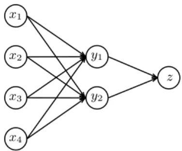
Lisa
Priscilla
Elvis Barack Michelle
Sasha Malia
hasChild hasChild hasChild hasChild marriedTo marriedTo
Fig. 1. Example KB
Definition 14 (Prediction of a rule): The predictions P of a rule B ⇒ h in a KB K are the head atoms of all instantiations of the rule where the body atoms appear in K. We write K ∧ (B ⇒ h) |= P . The predictions of a set of rules are the union of the predictions of each rule.
For example, consider the KB in Figure 1. The predictions of the rule marriedTo(x, y) ∧ hasChild(y, z) ⇒ hasChild(x, z) are hasChild(Priscilla, Lisa), hasChild(Elvis, Lisa), hasChild(Barack, Sasha), hasChild(Barack, Malia), hasChild(Michelle, Sasha), hasChild(Michelle, Malia). This is useful, because two of these facts are not yet in the KB.
Logic. From a logical perspective, all variables in a rule are implicitly universally quantified (over every entity defined in the KB). Thus, our example rule is more explicitly written as
∀x, y, z : marriedTo(x, y) ∧ hasChild(y, z) ⇒ hasChild(x, z)
It can be easily verified that such a rule is equivalent to the following disjunction: ∀x, y, z : ¬marriedTo(x, y) ∨ ¬hasChild(y, z) ∨ hasChild(x, z)
While every Horn rule corresponds to a disjunction with universally quantified variables, not every such disjunction corresponds to a Horn rule. Only those disjunctions with exactly one positive atom correspond to Horn rules. In prin-ciple, we could mine arbitrary disjunctions, and not just those that correspond to Horn rules. We could even mine arbitrary first-order expressions, such as ∀x : person(x) ⇒ ¬(underage(x) ∧ adult(x)). For simplicity, we stay with Horn rules in what follows, and point out when an approach can be generalized to disjunctions or arbitrary formulae.
3.2 Rule Mining
3.2.1 Inductive Logic Programming
We now turn to mining rules automatically from a KB. This endeavor is based on Inductive Reasoning. To reason by induction is to expect that events that always appeared together in the past will always appear together in the future. For example, inductive reasoning could tell us: “All life forms we have
seen so far need water. Therefore, all life forms in general need water.”. This is the fundamental principle of empirical science: the generalization of past experi-ences to a scientific theory. Of course, inductive reasoning can never deliver the logical certitude of deductive reasoning. This is illustrated by Bertrand Russel’s analogy of the turkey [61]: The turkey is fed every day by its owner, and so it comes to believe that the owner will always feed the turkey – which is true only until Christmas day. The validity and limitations of modeling the reality using inductive reasoning are a debated topic in philosophy of science. For more perspectives on the philosophical discussions, we refer the reader to [29] and [31]. In the setting of KBs, inductive reasoning is formalized as Inductive Logic Programming [57,63,51]:
Definition 15 (Inductive Logic Programming): Given a background knowl-edge B (in general, any first order logic expression; in our case: a KB), a set of positive example facts E+, and a set of negative example facts E−,
Induc-tive Logic Programming (ILP) is the task of finding an hypothesis h (in gen-eral, a set of first order logic expressions; in our case: a set of rules) such that ∀e+∈ E+ : B ∧ h |= e+ and ∀e−∈ E−: B ∧ h 6|= e−.
This means that the rules we seek have to predict all positive examples (they have to be complete), and they may not predict a negative example (they have to be correct ). For example, consider again the KB from Figure 1 as background knowledge, and let the sets of examples be:
E+= { isMarriedTo(Elvis, Priscilla), isMarriedTo(Priscilla, Elvis),
isMarriedTo(Barack, Michelle), isMarriedTo(Michelle, Barack)}
E−= { isMarriedTo(Elvis, Michelle), isMarriedTo(Lisa, Barack), isMarriedTo(Sasha, Malia)}
Now consider the following hypothesis:
h= {isMarriedTo(x, y) ⇒ isMarriedTo(y, x)}
This hypothesis is complete, as every positive example is a prediction of the rule, and it is correct, as no negative example is predicted.
The attentive reader will notice that the difficulty is now to correctly deter-mine the sets of positive and negative examples. In the ideal case the positive examples should contain any fact that is true in the real world and the negative examples contain any other fact. Thus, in a correct KB, every fact is a positive example.
Definition 16 (Rule Mining): Given a KB, Rule Mining is the ILP task with the KB as background knowledge, and every single atom of the KB as a positive example.
This means that the rule mining will find several rules, in order to explain all facts of the KB. Three problems remain: First, we have to define the set of negative examples (Section 3.2.2). Second, we have to define what types of rules we are interested in (Section 3.2.3). Finally, we have to adapt our mining to cases where the rule does not always hold (Section 3.2.4).
3.2.2 The Set of Negative Examples
Rule mining needs negative examples (also called counter-examples). The problem is that KBs usually do not contain negative information (Section 2.6). We can think of different ways to generate negative examples.
Closed World Assumption. The Closed World Assumption (CWA) says that any statement that is not in the KB is wrong (Section 2.4.1). Thus, under the Closed-World Assumption, any fact that is not in the KB can serve as a neg-ative example. The problem is that these may be exactly the facts that we want to predict. In our example KB from Figure 1, we may want to learn the rule marriedTo(x, y) ∧ hasChild(y, z) ⇒ hasChild(x, z). For this rule, the fact hasChild(Barack, Malia) is a counter-example. However, this fact is exactly what we want to predict, and so it would be a counter-productive counter-example. Open World Assumption. Under the Open-World Assumption (OWA), any fact that is not in the KB can be considered either a negative or a positive example (see again Section 2.4.1). Thus the OWA does not help in establish-ing counter-examples. Without counter-examples, we can learn any rule. For example, in our KB, the rule type(x, person) ⇒ marriedTo(x, Barack) has a single positive example (for x = Michelle), and no counter-examples under the Open World Assumption. Therefore, we could deduce that everyone is married to Barack.
Partial Completeness Assumption. Another strategy to generate negative examples is to assume that entities are complete for the relations they already have. For example, if we know that Michelle has the children Sasha and Malia, then we assume (much like Barack) that Michelle has no other children. If, in contrast, Barack does not have any children in the KB, then we do not conclude anything. This idea is called the Partial-Completeness Assumption (PCA) or the Local Closed World Assumption [25]. It holds trivially for functions (such as hasBirthDate), and usually [26] for relations with a high functionality (such as hasNationality). The rationale is that if the KB curators took the care to enter some objects for the relation, then they will most likely have entered all of them, if there are few of them. In contrast, the assumption does usually not hold for relations with low functionality (such as starsInMovie). Fortunately, relations usually have a higher functionality than their inverses (see Section 2.3.3). If that is not the case, we can apply the PCA to the object of the relation instead. Random Examples. Another strategy to find counter-examples is to generate random statements [50]. Such random statements are unlikely to be correct, and can thus serve as counter-examples. This is one of the methods used by DL-Learner [30]. As we shall see in Section 4.3.1, it is not easy to generate helpful random counter-examples. If, e.g., we generate the random negative example marriedTo(Barack,USA), then it is unlikely that a rule will try to predict this example. Thus, the example does not actually help in filtering out any rule. The challenge is hence to choose counter-examples that are false, but still reasonable. The authors of [55] describe a method to sample negative statements about
semantically connected entities by help of the PCA. We will also revisit the problem in the context of representation learning (Section 4.3.1).
3.2.3 The Language Bias
After solving the problem of negative examples, the next question is what kind of rules we should consider. This choice is called the language bias, because it restricts the “language” of the hypothesis. We have already limited ourselves to Horn Rules, and in practice we even restrict ourselves to connected and closed rules.
Definition 17 (Connected rules): Two atoms are connected if they share a variable, and a rule is connected if every non-ground atom is transitively con-nected to one another.
For example, the rule presidentOf(x, America) ⇒ hasChild(Elvis, y) is not connected. It is an uninteresting and most likely wrong rule, because it makes a prediction about arbitrary y.
Definition 18 (Closed rules): A rule is closed if every variable appears in at least two atoms.
For example the rule marriedTo(x, y) ∧ worksAt(x, z) ⇒ marriedTo(y, x) is not closed. It has a “dangling edge” that imposes that x works somewhere. While such rules are perfectly valid, they are usually less interesting than the more general rule without the dangling edge.
Finally, one usually imposes a limit on the number of atoms in the rule. Rules with too many atoms tend to be very convoluted [26]. That said, mining rules without such restrictions is an interesting field of research, and we will come back to it in Section 3.5.
3.2.4 Support and Confidence
One problem with classical ILP approaches is that they will find rules that apply to very few entities, such as marriedTo(x, Elvis) ⇒ hasChild(x, Lisa). To avoid this type of rules, we define the support of a rule:
Definition 19 (Support): The support of a rule in a KB is the number of positive examples predicted by the rule.
Usually, we are interested only in rules that have a support higher than a given threshold (say, 100). Alternatively, we can define a relative version of sup-port, the head coverage [25], which is the number of positive examples predicted by the rule divided by the number of all positive examples with the same rela-tion. Another problem with classical ILP approaches is that they will not find rules if there is a single counter-example. To mitigate this problem, we define the confidence:
Definition 20 (Confidence): The confidence of a rule is the number of posi-tive examples predicted by the rule (i.e., the support of the rule), divided by the number of examples predicted by the rule.
This notion depends on how we choose our negative examples. For instance, under the CWA, the rule marriedTo(x, y)∧hasChild(y, z) ⇒ hasChild(x, z) has a confidence of 4/6 in Figure 1. We call this value the standard confidence. Under the PCA, in contrast, the confidence for the example rule is 4/4. We call this value the PCA confidence. While the standard confidence tends to “punish” rules that predict many unknown statements, the PCA confidence will permit more such rules. We present in Appendix A the exact mathematical formula of these measures.
In general, the support of a rule quantifies its completeness, and the con-fidence quantifies its correctness. A rule with low support and high concon-fidence indicates a conservative hypothesis and may be overfitting, i.e. it will not gener-alize to new positive examples. A rule with high support and low confidence, in contrast, indicates a more general hypothesis and may be overgeneralizing, i.e., it does not generalize to new negative examples. In order to avoid these effects we are looking for a trade-off between support and confidence.
Definition 21 (Frequent Rule Mining): Given a KB K, a set of positive examples (usually K), a set of negative examples (usually according to an as-sumption above) and a language of rules, Frequent rule mining is the task of finding all rules in the language with a support and a level of confidence superior to given thresholds.
3.3 Rule Mining Approaches
Using substitutions (see Definition 13), we can define a syntactical order on rules: Definition 22 (Rule order): A rule R ≡ (B ⇒ h) subsumes a rule R0 ≡ (B0 ⇒ h0), or R is “more general than” R0, or R0 “is more specific than” R,
if there is a substitution σ such that σ(B) ⊆ B0 and σ(h) = h0. If both rules
subsume each other, the rules are called equivalent. For example, consider the following rules:
hasChild(x, y) ⇒ hasChild(z, y) (R0)
hasChild(Elvis, y) ⇒ hasChild(P riscilla, y) (R1)
hasChild(x, y) ⇒ hasChild(z, Lisa) (R2)
hasChild(x, y) ∧ marriedT o(x, z) ⇒ hasChild(z, y) (R3)
marriedT o(v1, v2) ∧ hasChild(v1, v3) ⇒ hasChild(v2, v3) (R4)
hasChild(x, y) ∧ marriedT o(z, x) ⇒ hasChild(z, y) (R5)
The rule R0is more general than the rule R1, because we can rewrite the variables
x and z to Elvis and P riscilla respectively. However R0 and R2 are
incompa-rable as we cannot choose to bind only one y and not the other in R0. The rules
R3, R4and R5are more specific than R0. Finally R3is equivalent to R4 but not
to R5.
Proposition 23 (Prediction inclusion): If a rule R is more general than a rule R0, then the predictions of R0 on a KB are a subset of the predictions of R. As a corollary, R0 cannot have a higher support than R.
This observation gives us two families of rule mining algorithms: top-down rule mining starts from very general rules and specializes them until they become too specific (i.e., no longer meet the support threshold). Bottom-up rule mining, in contrast, starts from multiple ground rules and generalizes them until the rules become too general (i.e., too many negative examples are predicted).
3.3.1 Top-Down Rule Mining
The concept of specializing a general rule to more specific rules can be traced back to [63] in the context of an exact ILP task (under the CWA). Such ap-proaches usually employ a refinement operator, i.e. a function that takes a rule (or a set of rules) as input and returns a set of more specific rules. For example, a refinement operator could take the rule hasChild(y, z) ⇒ hasChild(x, z) and produce the more specific rule marriedTo(x, y)∧hasChild(y, z) ⇒ hasChild(x, z). This process is iterated, and creates a set of rules that we call the search space of the rule mining algorithm. On the one hand, the search space should contain every rule of a given rule mining task, so as to be complete. On the other hand, the smaller the search space is, the more efficient the algorithm is.
Usually, the search space is pruned, i.e., less promising areas of the search space are cut away. For example, if a rule does not have enough support, then any refinement of it will have even lower support (Proposition 23). Hence, there is no use refining this rule.
AMIE. AMIE [25] is a top-down rule mining algorithm that aims to mine any connected rule composed of binary atoms for a given support and minimum level of confidence in a KB. AMIE starts with rules composed of only a head atom for all possible head atoms (e.g., ⇒ marriedTo(x, y)). It uses three refinement operators, each of which adds a new atom to the body of the rule.
The first refinement operator, addDanglingAtom, adds an atom composed of a variable already present in the input rule and a new variable.
Some refinements of: ⇒ hasChild(z, y) (Rh)
are:
hasChild(x, y) ⇒ hasChild(z, y) (R0)
marriedT o(x, z) ⇒ hasChild(z, y) (Ra)
marriedT o(z, x) ⇒ hasChild(z, y) (Rb)
The second operator, addInstantiatedAtom, adds an atom composed of a vari-able already present in the input rule and an entity of the KB.
Some refinements of: ⇒ hasChild(P riscilla, y) (R0 h)
are:
hasChild(Elvis, y) ⇒ hasChild(P riscilla, y) (R1)
hasChild(P riscilla, y) ⇒ hasChild(P riscilla, y) (R>)
The final refinement operator, addClosingAtom, adds an atom composed of two variables already present in the input rule.
Some refinements of: marriedT o(x, z) ⇒ hasChild(z, y) (Ra)
are:
hasChild(x, y) ∧ marriedT o(x, z) ⇒ hasChild(z, y) (R3)
marriedT o(z, y) ∧ marriedT o(x, z) ⇒ hasChild(z, y) (Rα)
marriedT o(x, z) ∧ marriedT o(x, z) ⇒ hasChild(z, y) (R2 a)
As every new atom added by an operator contains at least a variable present in the input rule, the generated rules are connected. The last operator is used to close the rules (for example R3), although it may have to be applied several
times to actually produce a closed rule (cf. Rules Rα or R2a).
The AMIE algorithm works on a queue of rules. Initially, the queue contains one rule of a single head atom for each relation in the KB. At each step, AMIE dequeues the first rule, and applies all three refinement operators. The resulting rules are then pruned: First, any rule with low support (such as R⊥) is discarded.
Second, different refinements may generate equivalent rules (using the closing operator on R0 or Ra, e.g., generates among others two equivalent “versions”
of R3). AMIE prunes out these equivalent versions. AMIE+ [26] also detects
equivalent atoms as in R> or R2aand rewrites or removes those rules. There are
a number of other, more sophisticated pruning strategies that estimate bounds on the support or confidence. The rules that survive this pruning process are added to the queue. If one of the rules is a closed rule with a high confidence, it is also output as a result. In this way, AMIE enumerates the entire search space. The top-down rule mining method is generic, but its result depends on the initial rules and on the refinement operators. The operators directly impact the language of rules we can mine (see Section 3.2.3) and the performance of the method. We can change the refinement operators to mine a completely different language of rules. For example, if we don’t use the addInstantiatedAtom oper-ator, we restrict our search to any rule without instantiated atoms, which also drastically reduce the size of the search space6.
Apriori Algorithm. There is an analogy between top-down rule mining and the Apriori algorithm [1]. The Apriori algorithm considers a set of transactions (sales, products bought in a supermarket), each of which is a set of items (items bought together, in the supermarket analogy). The goal of the Apriori algorithm is to find a set of items that are frequently bought together.
These are frequent patterns of the form P ≡ I1(x) ∧ · · · ∧ In(x), where I(t) is
in our transaction database if the item I has been bought in the transaction t. Written as the set (called an “itemset”) P ≡ {I1, . . . , In}, any subset of P forms
a “more general” itemset than P , which is at least as frequent as P . The Apriori algorithm uses the dual view of the support pruning strategy: Necessarily, all patterns more general than P must be frequent for P to be frequent7. The
6
Let |K| be the number of facts and |r(K)| the number of relations in a KB K. Let d be the maximal length of a rule. The size of the search space is reduced from O(|K|d)
to O(|r(K)|d) when we remove the addInstantiatedAtom operator.
7
refinement operator of the Apriori algorithm takes as input all frequent itemsets of size n and generate all itemsets of size n + 1 such that any subset of size n is a frequent itemset. Thus, Apriori can be seen as a top-down rule mining algorithm over a very specific language where all atoms are unary predicates.
The WARMR algorithm [13], an ancestor of AMIE, was the first to adapt the Apriori algorithm to rule mining over multiple (multidimensional) relations.
3.3.2 Bottom-Up Rule Mining
As the opposite of a refinement operator, one can define a generalization operator that considers several specific rules, and outputs a rule that is more general than the input rules. For this purpose, we will make use of the ob-servation from Section 3.1 that a rule b1 ∧ ... ∧ bn ⇒ h is equivalent to
the disjunction ¬b1 ∨ · · · ∨ ¬bn ∨ h. The disjunction, in turn, can be
writ-ten as a set {¬b1, . . . , ¬bn, h} – which we call a clause. For example, the rule
marriedTo(x, y) ∧ hasChild(y, z) ⇒ hasChild(x, z) can be written as the clause {¬marriedTo(x, y), ¬hasChild(y, z), hasChild(x, z)}. Bottom-up rule mining ap-proaches work on clauses. Thus, they work on universally quantified disjunctions – which are more general than Horn rules. Two clauses can be combined to a more general clause using the “least general generalization” operator [57]: Definition 24 (Least general generalization): The least general generaliza-tion (lgg) of two clauses is computed in the following recursive manner:
– The lgg of two terms (i.e., either entities or variables) t and t0 is t if t = t0 and a new variable xt/t0 otherwise.
– The lgg of two negated atoms is the negation of their lgg.
– The lgg of r(t1, . . . , tn) and r(t01, . . . , t0n) is r(lgg(t1, t01), . . . , lgg(tn, t0n)).
– The lgg of a negated atom with a positive atom is undefined. – Likewise, the lgg of two atoms with different relations is undefined.
– The lgg of two clauses R and R0is the set of defined pair-wise generalizations:
lgg(R, R0) = {lgg(li, l0j) : li∈ R, lj0 ∈ R
0, and lgg(l
i, l0j) is defined}
For example, let us consider the following two rules:
hasChild(M ichelle, Sasha) ∧ marriedT o(M ichelle, Barack) ⇒ hasChild(Barack, Sasha) (R) hasChild(M ichelle, M alia) ∧ marriedT o(M ichelle, x)
⇒ hasChild(x, M alia) (R0)
In the form of clauses, these are
{¬hasChild(M ichelle, Sasha), ¬marriedT o(M ichelle, Barack), hasChild(Barack, Sasha)} (R) {¬hasChild(M ichelle, M alia), ¬marriedT o(M ichelle, x),
Now, we have to compute the lgg of every atom of the first clause with every atom of the second clause. As it turns out, there are only 3 pairs where the lgg is defined:
lgg(¬hasChild(M ichelle, Sasha), ¬hasChild(M ichelle, M alia)) = ¬lgg(hasChild(M ichelle, Sasha), hasChild(M ichelle, M alia)) = ¬hasChild(lgg(M ichelle, M ichelle), lgg(Sasha, M alia)) = ¬hasChild(M ichelle, xSasha/M alia)
lgg(¬marriedT o(M ichelle, Barack), ¬marriedT o(M ichelle, x)) = ¬marriedT o(M ichelle, xBarack/x)
lgg(hasChild(Barack, Sasha), hasChild(x, M alia)) = hasChild(xBarack/x, xSasha/M alia)
This yields the clause
{¬hasChild(M ichelle, xSasha/M alia), ¬marriedT o(M ichelle, xBarack/x),
hasChild(xBarack/x, xSasha/M alia)}
This clause is equivalent to the rule
hasChild(M ichelle, x) ∧ marriedT o(M ichelle, y) ⇒ hasChild(x, y)
Note that the generalization of two different terms in an atom should result in the same variable as the generalization of these terms in another atom. In our example, we obtain only two new variables xSasha/M aliaand xBarack/x. In this
way, we have generalized the two initial rules to a more general rule. This can be done systematically with an algorithm called GOLEM.
GOLEM. The GOLEM/RLGG algorithm [51] creates, for each positive example e ∈ E+, the rule B ⇒ e, where B is the background knowledge. In our case, B is
the entire KB, and so a very long conjunction of facts. The algorithm will then generalize these rules to shorter rules. More precisely, the relative lgg (rlgg) of a tuple of ground atoms (e1, . . . , en) is the rule obtained by computing the lgg of
the rules B ⇒ e1, ..., B ⇒ en. We will call a rlgg valid if it is defined and does
not predict any negative example.
The algorithm starts with a randomly sampled pair of positive examples (e1, e2) and selects the pair for which the rlgg is valid and predicts (“covers”)
the most positive examples. It will then greedily add positive examples, chosen among a sample of “not yet covered positive examples”, to the tuple – as long as the corresponding rlgg is valid and covers more positive examples. The resulting rule will still contain ground atoms from B. These are removed, and the rule is output. Then the process starts over to find other rules for uncovered positive examples.
Progol and others. More recent ILP algorithms such as Progol [49], HAIL [59], Imparo [36] and others [88,34] use inverse entailment to compute the hypothesis