ecoinvent: Energy Supply
Life Cycle Inventories for the Nuclear and Natural Gas Energy Systems,
and Examples of Uncertainty Analysis
Roberto Dones1*, Thomas Heck1, Mireille Faist Emmenegger2 and Niels Jungbluth2 1 Paul Scherrer Institute (PSI), Systems/Safety Analysis, CH-5232 Villigen PSI, Switzerland
2 ESU-services, environmental consultancy for business and authorities, Kanzleistrasse 4, CH-8610 Uster, Switzerland
* Corresponding author ([email protected])
tory data should reconsider production and transport from Rus-sia, as it is a major producer and exporter to Europe.
The calculated ranges of uncertainty factors in ecoinvent pro-vide useful information but they are more indications of uncer-tainties rather than strict 95% intervals, and should therefore be applied carefully.
Keywords: ecoinvent; electricity; gas combined cycle; industrial gas; life cycle inventory; natural gas system; nuclear fuel cycle; nuclear system; Switzerland; uncertainty
DOI: http://dx.doi.org/10.1065/lca2004.12.181.2 Abstract
Goal, Scope and Background. The energy systems included in
the ecoinvent database v1.1 describe the situation around year 2000 of Swiss and Western European power plants and boilers with the associated energy chains. The addressed nuclear sys-tems concern Light Water Reactors (LWR) with mix of open and closed fuel cycles. The system model 'Natural Gas' describes production, distribution, and combustion of natural gas.
Methods. Comprehensive life cycle inventories of the energy
sys-tems were established and cumulative results calculated within the ecoinvent framework. Swiss conditions for the nuclear cycle were extrapolated to major nuclear countries. Long-term radon emissions from uranium mill tailings have been estimated with a simplified model. Average natural gas power plants were ana-lysed for different countries considering specific import/export of the gas, with seven production regions separately assessed. Uncertainties have been estimated quantitatively.
Results and Discussion. Different radioactive emission species
and wastes are produced from different steps of the nuclear cy-cle. Emissions of greenhouse gases from the nuclear cycle are mostly from the upstream chain, and the total is small and de-creasing with inde-creasing share of centrifuge enrichment. The results for natural gas show the importance of transport and low pressure distribution network for the methane emissions, whereas energy is mostly invested for production and long-dis-tance pipeline transportation. Because of significant differences in power plant efficiencies and gas supply, country specific av-erages differ greatly.
Conclusion. The inventory describes average worldwide supply
of nuclear fuel and average nuclear reactors in Western Europe. Although the model for nuclear waste management was extrapo-lated from Swiss conditions, the ranges obtained for cumulative results can represent the average in Europe. Emissions per kWh electricity are distributed very differently over the natural gas chain for different species. Modern combined cycle plants show better performance for several burdens like cumulative green-house gas emissions compared to average plants.
Recommendation and Perspective. Comparison of
country-spe-cific LWRs or LWR types on the basis of these results is not recommended. Specific issues on different strategies for the nu-clear fuel cycle or location-specific characteristics would require extension of analysis.
Results of the gas chain should not be directly applied to areas other than those modelled because emission factors and energy requirements may differ significantly. A future update of
inven-Introduction
Fossil and nuclear energy systems dominate most of the elec-tricity mixes of European countries. Fossil fuels are provid-ing the heatprovid-ing services predominantly. For the ecoinvent database all non-renewable systems of importance have been assessed, namely: hard coal and lignite (Röder et al. 2004), oil (Jungbluth 2004), natural and industrial gases (Faist Emmenegger et al. 2003), and nuclear (Dones 2003). This paper presents the nuclear cycle and, as example for fossil systems, the natural gas energy system. Only electricity pro-duction is addressed here, although the database contains also gas boilers as well as combined heat and power plants (CHP) for industry and buildings. CHP fuelled by natural gas and oil are addressed in (Heck 2004), whereas wood CHPs are in (Bauer 2003). An English summary of all en-ergy systems addressed in ecoinvent is in (Dones et al. 2004).
1 Nuclear power
1.1 Goal, scope and background
The nuclear fuel cycles associated with power generation at Light Water Reactors (LWR) currently installed in Western Europe (UCTE) have been modelled in ecoinvent. The focus was on the two units of the 1000 MW class operating in Switzerland: Gösgen Pressurized Water Reactor (PWR) and Leibstadt Boiling Water Reactor (BWR). The conditions of the fuel cycles for the Swiss reactors have been assessed, modelled, and extrapolated to France, Germany, and UCTE as average for Western Europe. Besides describing the nu-clear cycle as such, the assessment served the estimation of cumulative environmental burdens of European electricity mixes, along with other electricity systems in ecoinvent (Frischknecht & Faist Emmenegger 2003).
1.2 Life Cycle Inventory
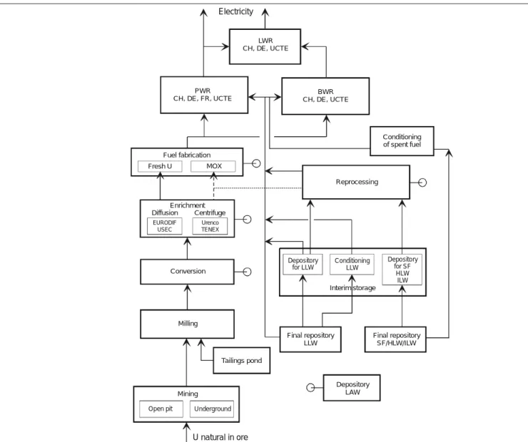
Fig. 1 gives a schematic overview of the modelled nuclear
fuel cycles. The arrows with continuous line give the direc-tion of the environmental burdens to be added up to give cumulative burdens associated with the unit of electricity. Information is provided here only on main assumptions con-cerning the nuclear cycle (front-end, power plant, back-end) and for those stages that contribute meaningfully to cumula-tive burdens, although with different environmental profiles, i.e. mining/milling, enrichment, power plant, and reprocessing. Besides the use of enriched uranium originating from natu-ral uranium ore (herewith named fresh U), recycling of plu-tonium from reprocessing and of depleted uranium from enrichment in mixed-oxide (MOX) fuel elements has been modelled estimating the equilibrium production of pluto-nium in the reactor. Thus, both open (no recycling) and closed fuel cycles are taken into account. The highly enriched
nium from dismantled warheads mixed with recycled ura-nium from spent fuel to make the so-called 'RepU' fuel ele-ments has been accounted for as uranium from natural sources, i.e. as it were enriched for direct use for civil pur-poses. For the static approach applied in ecoinvent, the plu-tonium and the depleted uranium are not loaded with the environmental burdens from the steps producing them. However, all cumulative burdens from reprocessing are at-tributed to the processed spent fuel and all cumulative bur-dens from the enrichment step are attributed to the produc-tion of enriched uranium. The flows of plutonium from reprocessing and depleted uranium from enrichment are rep-resented by dotted lines in Fig. 1.
For each modelled production process, a basic dataset to describe infrastructure (construction and decommissioning, were applicable) has been defined. The contaminated wastes from decommissioning are attributed to the operation of the facility rather than to the infrastructure dataset. Four
U natural in ore Electricity Centrifuge EURODIF USEC Urenco TENEX Mining Open pit Underground
Depository for LLW Conditioning LLW Final repository SF/HLW/ILW Final repository LLW Conditioning of spent fuel PWR CH, DE, FR, UCTE BWR CH, DE, UCTE LWR CH, DE, UCTE Fuel fabrication Fresh U MOX Tailings pond Enrichment Milling Conversion Reprocessing Interim storage Depository for SF HLW ILW Depository LAW Diffusion
BWR = Boiling Water Reactor; PWR = Pressurized Water Reactor; LWR = Light Water Reactor; CH = Switzerland; DE = Germany; FR = France; UCTE = Union for the Co-ordination of Transmission of Electricity; LAW = Low Active Waste; LLW = Low Level Waste; ILW = Intermediate Level Waste; HLW = High Level Waste; SF = Spent Fuel; U = Uranium
different classes of radioactive wastes have been modelled, namely mill tailings, other low active wastes (LAW) in near-surface depositories, low and medium short-lived waste (LLW), and high and intermediate long-lived radioactive waste including spent fuel (H/ILW and SF), the last two types to be disposed of in deep geological repositories.
The modelling of uranium mining includes open pit and under-ground mining but no chemical extraction (the latter makes about 30% of the total current yearly production, from statis-tics). Although mostly based on available literature of the early 1980s on conventional mining in the USA, and thus not fully reflecting different conditions for other countries, the model-ling of mining and milmodel-ling as a whole should still represent a practical picture of the uranium extraction industry suited for the goals of ecoinvent. The variability of the shares of different extraction processes over the years, the existence of large stocks of uranium extracted in the past, the availability of fuel from warheads as cited above, and the need to approximate lifetime conditions of uranium supply to the cycles more than snapshot conditions; all these elements make the definition of average shares somewhat arbitrary. Sensitivity analyses may serve to estimate the influence of the variation of key parameters on the cumulative results, but these analyses where beyond the scope of ecoinvent. Certainly, local impacts on groundwater from chemical mining deserve attention in future studies.
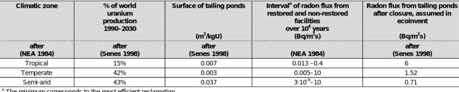
Uranium milling is important concerning the burdens from the tailing ponds, in particular the long-term emissions of ra-dioactive radon to air. Gaseous radon emissions are moni-tored to verify the performance of uranium mills, because of the carcinogenic risks associated with the exposure to the iso-tope Rn-222 and its progeny. This crucial aspect has been ad-dressed by developing a simple emission model using moder-ately conservative assumptions, as can be seen from Table 1 comparing the assumed radon fluxes with the ranges provided in (NEA 1984). Average figures on tailing ponds area, radon flux after closure and reclamation (when planned), and life-time production of natural uranium for the most important mills around the world were estimated after (Senes 1998, EPA 1983). The mills have been roughly categorized according to three climatic conditions. The climate zones are important for the different likely weathering patterns of the mill tailings and their effects on the radon flux (for example, an ice crust on top of the tailings stops emission, while cracking in dry condi-tions increases emissions). Considering an integration time of 80000 years, approximately corresponding to the half-life of the Rn-222 parent isotope Th-230 (radon is generated in equi-librium with the decay of Th-230 isotope), the long-term emis-sion of radon is estimated at about 3.5·107 kBq/kgU. This
in-tegration time was introduced on the one hand to reflect the reduction of flux from the tailing surface to values closer to natural backgrounds of uraniferous areas, on the other hand to match the time span of 60000 years considered in (Doka 2003) for the non-radioactive landfill models.
A modelling of long-term emissions (>100 years) to ground-water from tailings after closure of uranium mills could not be performed. Extrapolation of models used in (Doka 2003) for non-radioactive wastes was not easily possible because they have been developed for Swiss conditions and do not include radiological decay. The short-term (<100 years) emissions to groundwater have been roughly estimated using the average composition of a few US uranium mill tailings and assuming that of the amounts existing at the shutdown of the mill, 5% of highly soluble elements and 1% of other species will be released. The 100-year time set defined in ecoinvent is also roughly consistent with the 70-year surveillance and mainte-nance period following remediation, planned in the frame of the uranium mill tailings remedial action program of the US Department of Energy, applied in 24 US sites.1
Two commercial enrichment processes, diffusion and cen-trifuge, have been modelled each with two different facili-ties to take into account the great variability in energy in-tensity, type of supply of electricity, and cooling fluid. Because of their importance for key cumulative inventories, the main assumptions are here summarized:
1. The electricity supply of 2400 kWh per kg of separative work unit (SWU)2 to the diffusion Eurodif plant in Trica-stin (France) is directly from nuclear power plants on the same site. The facility is water-cooled.
2. The electricity supply to the only USEC diffusion plant still in operation, Paducah (USA), is directly from coal power plants. The assumed electricity intensity is 2600 kWh/kgSWU. The facility is still cooled with CFC-114, leaking at an assumed rate of about 0.02 kg/kgSWU (Trowbridge 1991).3
3. The electricity intensity for all centrifuge Urenco plants (Germany, The Netherlands, UK) is about 40 kWh/kgSWU (Urenco 2000), assuming supply from the UCTE grid. Since 2000, no CFC is used in Gronau (Germany) but R134a, leaking at an estimated small rate of 2.6·10–4 kg/kgSWU.
The same has been assumed for all Urenco plants.
Climatic zone % of world
uranium production 1990–2030
Surface of tailing ponds
(m2
/kgU)
Intervala
of radon flux from restored and non-restored
facilities
over 104 years
(Bq/m2
s)
Radon flux from tailing ponds after closure, assumed in
ecoinvent (Bq/m2 s) after (NEA 1984) after (Senes 1998) after (Senes 1998) (NEA 1984) after (Senes 1998) Tropical 15% 0.007 0.013 –0.4 6 Temperate 42% 0.003 0.005–10 1.52 Semi-arid 43% 0.037 3·10-6 –10 0.71 a
The minimum corresponds to the most efficient reclamation.
Table 1: Summary of the estimated average radon fluxes from uranium mill tailing ponds for three different climatic zones worldwide
1http://www.antenna.nl/wise/uranium/udusat1.html
2The separative work unit is the standard measure of the effort required to increase the grade of fissile isotope U-235.
3Similar value can be deduced from http://www.antenna.nl/wise/466/ 4631.html, retrieved in June 2003.
4. The electricity supply to TENEX (Russia) centrifuge plants is assumed to be from the CENTREL electricity mix. The electricity intensity as well as all other require-ments and emissions are arbitrarily assumed to be the double of Urenco's.
Two datasets describe the infrastructure of the Swiss units Gösgen and Leibstadt. These were used to represent similar reactors of the 1000 MW class in the countries with the high-est nuclear share in UCTE, i.e. France and Germany. How-ever, to represent the infrastructure use for operation of the several reactors of the 1300 MW class, appropriate scaling factors on the basis of actual average efficiency, fuel burn-ups, and capacity factors were applied. One dataset describes the Swiss PWR in case that only centrifuge enrichment from Urenco would be used, to characterize a representative nu-clear cycle for LWR with the minimum electricity requirement. The utilization of fuel elements of all sorts for the supply of one unit of electric energy to the grid can be calculated as: Fuel requirement in [kgU/kWh] =
{Burn-up in [MWth·d/kgU] × 24 × 1000 × Net efficiency}–1
where the burn-up in MWth·day is the thermal energy devel-oped in 24 hours operation at rated power.
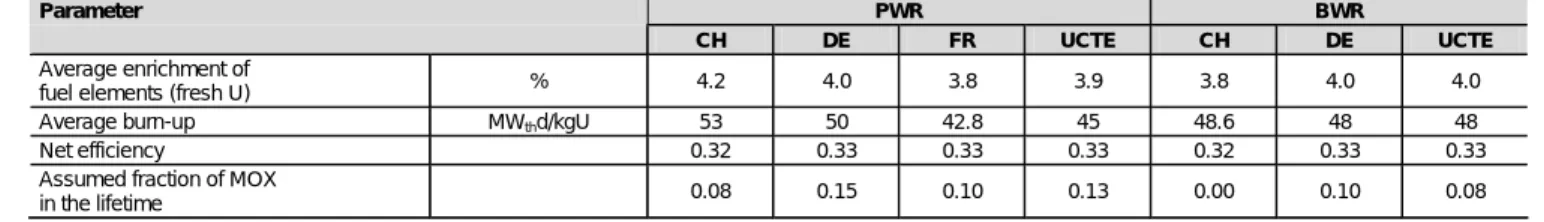
In 40 year lifetime, all MOX fuel elements loaded in Gösgen will cover approximately 8% of the fuel requirements and total energy production. In Leibstadt no MOX fuel element is used yet, for that all fuel is assumed to be from fresh uranium. For the definition of the reference average burn-up for both units, information from the operators on the finally discharged fuel elements in the years 2000 to 2002 has been used. Key factors assumed in the study are reported in Table 2. Consid-ering that in past years the enrichment and burn-up for the two plants were smaller and that it may increase in the future up to 55 MWth·d/kgHM (Heavy Metal, uranium if no MOX is used), the assumptions should approximately reflect aver-age conditions over the lifetime of the plants. For calculating fuel use in UCTE PWR and BWR, the values for CH, DE and FR are weighted with their electricity production.
The current policies for the reprocessing of all (assumed for France) or partial (Switzerland, Germany) spent fuel from the entire lifetime of the installed plants have been considered, although there might be slight contradiction for the domestic plutonium balance (total reprocessed versus total employed in MOX fuel). The radioactive emissions to air and water from each nuclear power plant in UCTE have been taken from one comprehensive publication of the European Union (Van der Stricht & Janssens 2001). The time interval considered for averaging the emissions is 1995–1999, but up to year 2002 for the Swiss units (BAG 1996–2003). Typically, a BWR di-rectly emits during operation more aerosols than a PWR, be-cause of the different characteristics of the primary circuit of
the reactor. For the discussion of results, the radioactive emis-sions to air have been grouped (un-weighted) into: radon; other noble gases plus H-3 and C-14; aerosols; and, actinides. The emissions to water have been grouped (un-weighted) into: ra-dium; tritium; mixed nuclides; and, actinides.
The amounts of radioactive waste from the operation and decommissioning of power plants are conservatively based on Swiss data from the mid 1990s. The most recent assess-ment on decommissioning performed by the operators of the PWR Gösgen was not available, but it is expected that the radioactive wastes from decommissioning of the plant would reduce by approximately one third compared to the values inputted in the database.
Two possible alternatives for the treatment of spent fuel have been described: reprocessing and conditioning by encapsula-tion of untreated spent fuel for direct disposal. In ecoinvent, the elementary flows for reprocessing and conditioning are allo-cated to the spent fuel. The waste products from reprocessing and the conditioned radioactive waste from the operation of power plants are transported to the Swiss interim storage. Key data for reprocessing have been taken from an environ-mental report for the French facility in La Hague (Cogema 1998). The report does not provide single radioactive iso-topes emitted but classes. Releases of C-14 and plutonium isotopes to air could be extrapolated or reconstructed from older references.
The new Swiss concept for a partially reversible geological repository in opalinus clay for high and intermediate long-lived radioactive waste (H/ILW) as well as spent fuel (SF) con-ditioned without reprocessing (Nagra 2002a, Nagra 2002b) has been modelled in ecoinvent. The assessment includes the amount of overburden, the material and energy uses for min-ing the tunnels, placmin-ing the wastes, and eventually sealmin-ing the repository. The radioactive waste inventory considers the cur-rent policy for recycling 40% of the total Swiss spent fuel pro-duced over 40 years operation of the power plants, leaving the rest to conditioning. The geological final repository for low and medium short-lived radioactive waste (LLW) is based on data from the concept developed in mid 1980s (Nagra 1985a, Nagra 1985b), because no newer concept is available yet.
A detailed description of the current waste streams and amounts from reprocessing back to the Swiss nuclear power plant operators was not at hand during the work. There-fore, the coherent set developed for the previous versions of this LCI study, was basically maintained, which can be seen as a conservative way to deal with the modeling because it ends up to maximize the volumes of the waste. Anyway, the contribution from the geological repositories to total inven-tories is relatively small due to the typically small waste vol-umes per unit of electricity.
PWR BWR
Parameter
CH DE FR UCTE CH DE UCTE
Average enrichment of
fuel elements (fresh U) % 4.2 4.0 3.8 3.9 3.8 4.0 4.0 Average burn-up MWthd/kgU 53 50 42.8 45 48.6 48 48
Net efficiency 0.32 0.33 0.33 0.33 0.32 0.33 0.33 Assumed fraction of MOX
in the lifetime 0.08 0.15 0.10 0.13 0.00 0.10 0.08
The risk studies performed by Nagra (e.g. Nagra 2002a) aim at demonstrating that the various man-made and natural pas-sive barriers interposed between the conditioned radioactive wastes and the biosphere are effective to attenuate and delay the release to the biosphere of not yet decayed radioisotopes, which will occur between 104–107 years from the sealing of
the repositories. The related maximum individual dose to hu-mans must remain, for Switzerland, below a threshold, fixed by the Swiss Nuclear Authority, at any time and for all possi-ble release scenarios. The time when the remaining released isotopes might have a peak in the biosphere is much longer (Nagra 2002a) than the time assumed in ecoinvent for the calculation of long-term releases from non-radioactive waste depositories (Doka 2003). Furthermore, it can be shown that even the amounts released over extremely long time remain very low when divided by the electricity production corre-sponding to the total deposited waste. Just as an example, of the few isotopic species that may reach the biosphere, in the
reference case analysed in (Nagra 2002a) the I-129 dose has a peak at about one million year from the sealing of the reposi-tory. The peak for all isotopes reaching the biosphere, which approximately equals the peak of I-129, is more than three orders of magnitude lower that the Swiss regulatory guideline threshold. Roughly assuming a constant dose of I-129 of the order of magnitude of its peak for one million year, the inte-gral of doses converted to emission would be of the same or-der of magnitude of the short-term emission of I-129 calcu-lated by ecoinvent. For all the above reasons, no release from the nuclear wastes in final geological repositories to the bio-sphere is accounted for in this LCI study.
1.3 Results and discussion
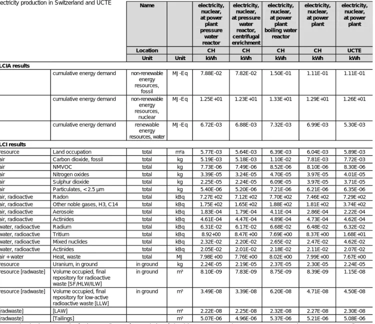
Table 3 shows selected cumulative LCI results and
cumula-tive energy demand for electricity production at the busbar of some modelled nuclear power plants and mixes.
Name electricity, nuclear, at power plant pressure water reactor electricity, nuclear, at pressure water reactor, centrifugal enrichment electricity, nuclear, at power plant boiling water reactor electricity, nuclear, at power plant electricity, nuclear, at power plant Location CH CH CH CH UCTE Unit Unit kWh kWh kWh kWh kWh LCIA results
cumulative energy demand non-renewable energy resources,
fossil
MJ-Eq 7.88E-02 7.82E-02 1.50E-01 1.11E-01 1.11E-01
cumulative energy demand non-renewable energy resources,
nuclear
MJ-Eq 1.25E+01 1.23E+01 1.33E+01 1.29E+01 1.26E+01
cumulative energy demand renewable energy resources, water
MJ-Eq 6.72E-03 6.88E-03 7.32E-03 6.99E-03 5.30E-03
LCI results
resource Land occupation total m²a 5.77E-03 5.64E-03 6.39E-03 6.04E-03 5.89E-03 air Carbon dioxide, fossil total kg 5.19E-03 5.18E-03 1.10E-02 7.81E-03 7.72E-03
air NMVOC total kg 7.73E-06 7.49E-06 8.52E-06 8.10E-06 8.30E-06 air Nitrogen oxides total kg 3.39E-05 3.24E-05 4.70E-05 3.97E-05 4.01E-05 air Sulphur dioxide total kg 2.25E-05 2.24E-05 6.09E-05 3.97E-05 3.71E-05 air Particulates, < 2.5 µm total kg 5.40E-06 5.20E-06 7.21E-06 6.21E-06 6.35E-06
air, radioactive Radon total kBq 7.27E+02 7.12E+02 7.70E+02 7.46E+02 7.29E+02 air, radioactive Other noble gases, H3, C14 total kBq 1.75E+02 1.65E+02 1.88E+02 1.81E+02 3.74E+02 air, radioactive Aerosole total kBq 1.83E-04 1.79E-04 4.11E-04 2.86E-04 2.22E-04 air, radioactive Actinides total kBq 4.61E-04 4.47E-04 4.89E-04 4.73E-04 4.62E-04 water, radioactive Radium total kBq 6.31E-02 6.17E-02 6.68E-02 6.48E-02 6.32E-02 water, radioactive Tritium total kBq 8.92+00 8.47E+00 7.69E+00 8.37E+00 1.68E+01 water, radioactive Mixed nuclides total kBq 2.32E-02 2.20E-02 2.65E-02 2.47E-02 4.62E-02 water, radioactive Actinides total kBq 2.05E-02 2.01E-02 2.18E-02 2.11E-02 2.07E-02 air + water Heat, waste total MJ 7.98E+00 7.76E+00 8.02E+00 7.99E+00 7.67E+00 resource Uranium, in ground in ground kg 2.24E-05 2.19E-05 2.37E-05 2.30E-05 2.24E-05 resource [radwaste] Volume occupied, final
repository for radioactive waste [SF/HLW/ILW]
in ground m³ 8.10E-09 7.83E-09 8.75E-09 8.39E-09 1.15E-08
resource [radwaste] Volume occupied, final repository for low-active radioactive waste [LLW]
in ground m³ 3.49E-08 3.39E-08 6.20E-08 4.71E-08 4.50E-08
[radwaste] [LAW] m³ 2.22E-08 2.25E-08 2.32E-08 2.27E-08 2.30E-08 [radwaste] [Tailings] m³ 5.07E-06 4.96E-06 5.37E-06 5.21E-06 5.08E-06 CH = Switzerland; UCTE = Union for the Co-ordinaton of Transmission of Electricity; LAW = Low Active Waste; LLW = Low Level Waste; ILW = Intermediate
Level Waste; HLW = High Level Waste; SF = Spent Fuel
Table 3: Selected cumulative LCI results and cumulative energy demand for electricity production at PWR and BWR in Switzerland, and average nuclear
0 1 2 3 4 5 6 7 8 Mini ng Millin g Conve rsion Enri chm ent Fuel fabr icati on BWR CH Repr oces sing Inte rim stor age Cond itioni ng Repos itory LLW Repo sito ry S F, H -ILW GH G g( C O2 -equ iv . )/ k W h Others N2O CH4 CO2
Upstream PWR Waste management
0 1 2 3 4 5 6 7 8 Mini ng Milli ng Conv ers ion Enric hme nt Fuel fabri catio n BWR CH Repr oces sing Inter im s torag e Con ditio ning Repos itory LL W Rep osito ry SF , H-IL W GH G g( C O2 -equ iv . )/ k W h Others N2O CH4 CO2
Upstream BWR Waste management
The total uranium ore consumption has been calculated for all analysed cycles in the interval 2.0·10–5 to 2.4·10–5 kgU
nat/kWh,
depending upon the assumed burn-up, average enrichment of fresh fuel, and source of enrichment services.
The total waste heat is prevalently (>95%) from the opera-tion of the power plant. The way the waste heat has been inventoried is such that the difference between cumulative value and direct output of waste heat from a power plant may serve as a measure of the total energy uses throughout the cycle. Assuming a reference efficiency of conversion ther-mal energy to electricity of 35% to express the total energy requirements in electricity-equivalent units, the calculated range for these is between 0.011 kWh use per kWh pro-duced at Swiss PWR in the hypothesis of centrifuge enrich-ment only up to 0.050 kWh use per kWh produced at French PWR. The average for current UCTE nuclear chains is 0.035 kWh use per kWh produced at LWRs.
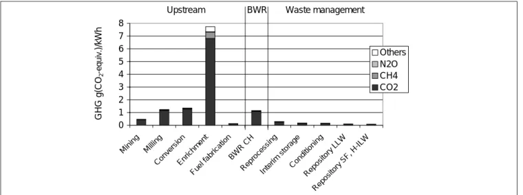
The range of the total greenhouse gas (GHG) emissions for the modelled European nuclear energy chains associated with LWRs is between 5 and 12 g CO2-equiv./kWh, for 100 year
time horizon after (IPCC 2001). The differences can be attrib-uted mostly to the North American diffusion facility Paducah, assumed to supply 13% of total enrichment services for the Swiss BWR and none to the Swiss PWR (Fig. 2 vs. Fig. 3). The emissions of CFC-114 (included in 'Others') are small com-pared to CO2. The contribution from centrifuge enrichment to total GHG is very low due to its much lower energy inten-sity compared to diffusion, and negligible GHG stems from the French diffusion plant. The GHG emissions from other steps are due to the use of fossil energy sources either directly or through the electricity mixes. The waste management, also including all operations for final geological repositories, gives only minor contribution to total GHG from the cycle.
Fig. 4 shows the radioactive air emissions from the cycles
for the Swiss PWR. The shape and values for corresponding categories for the Swiss BWR cycle do not change signifi-cantly. Radon stems from mining and milling, where the predominant part is the long-term emission from mill tail-ings. Noble gases originate from the power plant and re-processing; the emission from reprocessing per unit mass of
Fig. 2: Contributions of single species to total GHG emission per kWh from single steps in the nuclear fuel cycle of the Swiss BWR
heavy metal is nearly three orders of magnitude higher than for the unit mass of uranium in LWR fuel elements. The LWR and reprocessing are the major contributors to total release of aerosols. The results for radioactive emissions to water show typically higher tritium release per kWh from the PWR, and higher mixed nuclides release from the BWR. Table 3 shows the volumes per kWh of the four categories of radioactive solid wastes from the Swiss PWR and BWR cy-cles. BWRs produce typically more LLW from operation and decommissioning than PWRs. Also the H/ILW volume is higher, due to the slightly higher mass of spent fuel per kWh.
1.4 Conclusion
The results of the inventory for ecoinvent data v1.1 describe the current average nuclear system in Western Europe, although several items like the radioactive waste volume inventories are not accounting for recent decrement trends. The effects of the extrapolation of the Swiss waste management data to France and Germany should not meaningfully increase the
uncertainties in the cumulative results for those countries, nor for UCTE average conditions. Therefore, substantial changes in the cumulative results for the nuclear cycle are not expected if local conditions were fully represented, with the exception of the contributions to total radioactive emissions from re-processing in the case it would not be performed. The GHG emission of 5 g CO2-equiv./kWh calculated for the chain with
centrifuge enrichment only can be assumed representative for near future nuclear cycles for LWRs. The GHG calculated for mixes of LWR in UCTE countries varies between 8 and 11 g CO2-equiv./kWh.
2 Natural Gas 2.1 Introduction
The inventory analysis 'Natural Gas' describes the produc-tion, distribution and combustion of natural gas for indus-trial and domestic applications in Switzerland and Western Europe. The model includes gas field exploration, natural gas production, natural gas purification, long distance trans-port, regional distribution and combustion in boilers and power plants. In this study, natural gas power plants and industrial gas power plants are treated separately.
2.2 Goal, scope and background
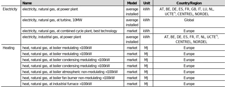
The database covers electricity generation as well as heating systems (Table 4). In order to represent current electricity production in Europe, average installed natural gas and in-dustrial gas power plants have been considered. Addition-ally, a dataset for the most advanced combined cycle tech-nology currently available at the market has been included. The datasets 'electricity, natural gas, at power plant' refer to average natural gas power plants operating around year 2000 (which is the reference year for the whole gas system model). For electricity production at a standard gas turbine
Fig. 4: Radioactive emissions to air from the upstream, power plant, and
downstream parts per kWh of the Swiss PWR nuclear fuel cycle
Name Model Unit Country/Region
electricity, natural gas, at power plant average installed
kWh AT, BE, DE, ES, FR, GB, IT, LU, NL, UCTE*), CENTREL, NORDEL electricity, natural gas, at turbine, 10MW average
installed
kWh Global
electricity, natural gas, at combined cycle plant, best technology market kWh Europe Electricity
electricity, industrial gas, at power plant average installed
kWh AT, BE, DE, ES, FR, IT, NL, UCTE*), CENTREL, NORDEL heat, natural gas, at boiler modulating <100kW market MJ Europe heat, natural gas, at boiler modulating >100kW market MJ Europe heat, natural gas, at boiler condensing modulating <100kW market MJ Europe heat, natural gas, at boiler condensing modulating >100kW market MJ Europe heat, natural gas, at boiler atmospheric non-modulating <100kW market MJ Europe heat, natural gas, at boiler fan burner non-modulating <100kW market MJ Europe Heating
heat, natural gas, at industrial furnace >100kW market MJ Europe *)
UCTE as of year 2000 i.e. excluding CENTREL countries.
AT = Austria, BE = Belgium, DE = Germany, ES = Spain, FR = France, GB = Great Britain, IT = Italy, LU = Luxembourg, NL = The Netherlands, UCTE = Union for the Co-ordination of Transmission of Electricity, CENTREL = Central European power association, NORDEL = Nordic countries power association
of about 10 MWe, only one dataset describing generic world-wide conditions is provided. Besides natural gas power plants, industrial gas power plants are described in separate datasets. Coke oven gas is a by-product of coke making, whose production is described in (Röder et al. 2004). The burdens from coking are allocated to the products accord-ing to their heataccord-ing value. Blast furnace gas is a by-product of the steel production; the burdens from the process are all allocated to the produced pig iron, none to the produced gas. For natural gas heating systems, boilers with advanced technology available at the market around the year 2000 have been modelled.
2.3 Life cycle inventory
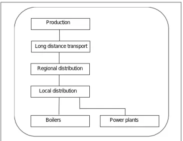
All process steps shown in Fig. 5 are included in the model. The natural gas upstream chain is divided into the follow-ing process steps: natural gas production (which includes exploration, production at field, purification), long-distance transportation, regional distribution, and local supply. These steps are explained in detail below.
• Natural gas exploration: Because drilling is in common for oil and gas extraction, the same emission and pro-duction factors per meter drilled borehole are used (Jungbluth 2004). Geophysical prospection is excluded due to negligible contributions to total requirements.
• Natural gas production: The requirements and emissions of natural gas production per cubic meter natural gas extracted are modelled for the following regions: North Sea (The Netherlands, Norway, Great Britain), Onshore Germany, Algeria, Russian Federation, Nigeria. If nec-essary (and possible) a regional distinction is made be-tween onshore and offshore production. Data are mostly based on environmental reports of companies operating in the modelled areas. Disposal of waste is mainly based on data from the North Sea (Norwegian production). In the system model, thermal and off-grid electric energy re-quired in natural gas production is provided by natural gas motors and turbines. The allocation for the combined oil and gas production is based on the lower heating value (net calorific value) of crude oil and natural gas.
• Natural gas purification: Natural gas is treated to elimi-nate water and oil, higher hydrocarbons, and sulphur. Sweet gas and sour gas are considered separately. Sour gas has an elevated content of sulphur and CO2. In
par-ticular the content of H2S is about 6 vol.% for sour gas.
• Long distance transportation: Energy requirements for compressor stations and gas leakages are considered as well as construction of pipelines and control flights along the pipelines. The compressors are driven by gas turbines fed with a share of the gas transported. A substantial share of Algerian natural gas is shipped as liquefied natu-ral gas (LNG). Compression and regasification as well as ship transport are included. Methane leakage rate is as-sumed 1.4% for the total average distance (6000 km) for the transmission of natural gas from the Russian Federa-tion (Zittel 1998) and about 0.026% per 1000 km pipe-line for the other producer countries (calculated on the basis of Reichert and Schön (2000) and Ruhrgas (2001)). For the LNG tanker transport from Algeria to Italy the leakage rate is 0.04% (Snam 1999). Energy use in the com-pressor stations of the pipelines is estimated 1.8% of trans-ported gas per 1000 km in Europe and of 2.7% per 1000 km for the Russian Federation. Energy use of the LNG freight ship is about 0.01 Nm3 per tkm (Snam 1999).
• Regional distribution and local supply: The model includes the construction of the gas pipelines usually operated with an over pressure of 0.1 to 1 bar. Gas leakages (0.02% on the high pressure level, additional 0.72% on the low pres-sure level for the Swiss supply situation (Liechti 2002, Re-ichert & Schön 2000, Seifert 1998)) and land use during construction and operation are considered.
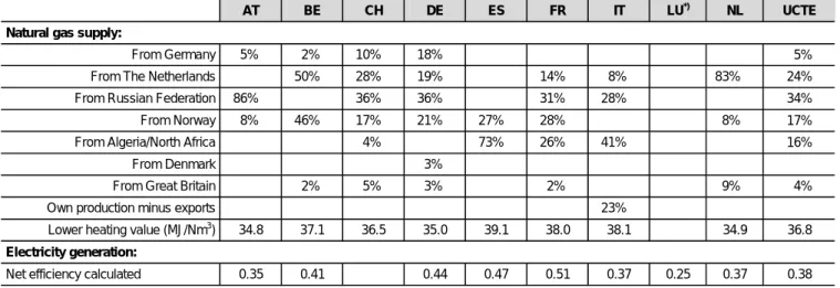
Table 5 shows key factors for the natural gas supply and for
the average natural gas power plants in UCTE. Natural gas sold in a country is assumed to be a mix of its domestic production and imports. Exports are treated like domestic sales. The import structure is decisive for the gas transport distances and for the environmental burdens related to the upstream chain. The fuel used in the natural gas power plants is directly supplied by high pressure gas pipelines. For the modelling of average power plants in different countries and different regions, national average efficiencies of gas power plants are used (see Table 5). Heat production in combined heat and power (CHP) operation lowers the electric efficiency of the power plant. In order to consider heat supply, the na-tional average efficiency was corrected by an exergy factor for heat (Faist Emmenegger et al. 2003). If no large CHP power plants were considered, the electric net electric efficiency of UCTE natural gas power plants would be about 40%. If CHP is included, the uncorrected net electric efficiency (total net electricity production divided by total fuel burned) decreases to 36% and thus one would penalise CHP production. The exergy-corrected net electric efficiency lies in between (at 38%, see Table 5). The exergy-corrected efficiency has been used for countries for which appropriate data were available. Be-sides the countries shown, CENTREL, NORDEL, and Great Britain are included in the database. Switzerland has currently no large natural gas power plant. Nevertheless, the use of natu-ral gas in small cogeneration units is quite common in
Swit-Production
Long distance transport
Regional distribution
Local distribution
Boilers Power plants
zerland. Small heat and power cogeneration plants are treated in a separate chapter in ecoinvent (Heck 2004).
The modelled combined cycle power plant, representing the best current technology, has an assumed power rate of about 400 MWe (about 265 MWe from the gas turbine and about 135 MWe from the steam engine). Data from the new 400 MWe power plant Mainz-Wiesbaden (Germany) were used. According to the operators, this is (as of year 2001) the natu-ral gas power plant with the highest net electric efficiency (58.4%) worldwide (KMW 2002). Because the efficiency de-pends also on the local environmental temperature conditions, it was assumed that a comparable plant at an average loca-tion in Europe would have a net electric efficiency of about 57.5%. In reality, the efficiency depends also on the mode of operation (peak load management, combined heat and power supply). Different modes of operation have not been consid-ered, i.e. optimal electricity production was assumed. For modelling of heating systems it has been assumed that the small boilers (<100 kW) are connected to the low pres-sure distribution network and that the large boilers (>100 kW) are connected to the high pressure network. One new methodological aspect of the ecoinvent data is the quantitative consideration of data uncertainties. Fig. 6 illus-trates the relative frequency distribution of NOx emissions during operation of modern modulating condensing natural gas boilers. The example is based on about 400 measure-ment values (SVGW 2002). The variation is represented by an uncertainty factor in the database given as the square of the geometric standard deviation of the lognormal approxi-mation. At present, four statistical distributions for input data can be chosen in the ecoinvent software system, namely uniform, triangular, lognormal and normal distribution. Among these, the lognormal distribution is considered the best choice for non-negative values like the emission values shown. A normal distribution would be inappropriate in particular for broad distributions spanning one or more
or-AT BE CH DE ES FR IT LU*) NL UCTE
Natural gas supply:
From Germany 5% 2% 10% 18% 5%
From The Netherlands 50% 28% 19% 14% 8% 83% 24%
From Russian Federation 86% 36% 36% 31% 28% 34%
From Norway 8% 46% 17% 21% 27% 28% 8% 17%
From Algeria/North Africa 4% 73% 26% 41% 16%
From Denmark 3%
From Great Britain 2% 5% 3% 2% 9% 4%
Own production minus exports 23%
Lower heating value (MJ/Nm3) 34.8 37.1 36.5 35.0 39.1 38.0 38.1 34.9 36.8
Electricity generation:
Net efficiency calculated 0.35 0.41 0.44 0.47 0.51 0.37 0.25 0.37 0.38 *) For LU: UCTE gas assumed; 1997 power generation data (IEA 2001).
AT = Austria, BE = Belgium, CH = Switzerland, DE = Germany, ES = Spain, FR = France, IT = Italy, LU = Luxembourg, NL = The Netherlands, UCTE = Union for the Co-ordination of Transmission of Electricity
Table 5: Key parameters of analyzed natural gas supply (VSG 2001, BP Amoco 2001) and average natural gas power plants in UCTE; efficiencies based
on 1999 production data (IEA 2001)
Fig. 6: Normalised frequency distribution of NOx emissions from modulat-ing condensmodulat-ing natural gas boilers <100 kW, derived from measurements in (SVGW 2002). Solid line: Lognormal approximation. The vertical axis refers to the relative frequency of measured values per (mg/MJ) interval; it is normalised so that the integral over the lognormal curve is 1 (the heights of all bars add up to 0.5 because each bar covers an interval of 2 mg/MJ)
ders of magnitude because it would reach out to the un-physical negative side of values. The lognormal distribution is used for all unit processes in ecoinvent (Frischknecht et al. 2004) i.e. for all unit processes in the gas chain as well. An uncertainty estimate based on a lot of measurements as shown in Fig. 6 could be performed only for NOx and CO emissions of natural gas boilers. In most cases, uncertainties in ecoinvent were either estimated from information avail-able in the literature or derived from basic uncertainty esti-mates and pedigree factors as described in the ecoinvent methodology (Frischknecht et al. 2004).
2.4 Results and discussion
The discussion of results focuses on natural gas supply and natural gas power plants because of their importance for electricity supply in Europe.
Fig. 7 shows a graphical analysis of the share of different
production stages of the gas supplied to the consumer at the Swiss low pressure network. A major part of the selected flows arises during the production (exploration, field pro-duction and purification) of natural gas. Energy requirements are mostly due to production and long-distance transport; distribution uses partly the pressure built up during the long-distance transport. Methane leakages occur for the most part in the transport from the Russian Federation and in the low pressure distribution network. Carbon dioxide is emitted from all stages of the upstream chain, mainly in the long distance transportation and in the exploration/field produc-tion, similar to the repartition of energy requirements along the production stages. Sulphur dioxide emissions are mainly caused during the gas desulphurisation and are therefore high for countries with sour gas.
Table 6 shows selected cumulative results for electricity
gen-eration at average natural gas power plants in different UCTE countries.
The country averages of the cumulative CO2 emissions of natu-ral gas power plants in Europe range from 460 to 930 g/kWhe.
Total greenhouse gas emissions (i.e. including CO2, CH4,
N2O and other greenhouse gases in the chain) range from
about 485 to about 990 g CO2-equiv./kWhe (100 year time
horizon). The differences are essentially determined by the country-specific average efficiencies, which depend on dif-ferent technologies (share of steam power plants, gas
tur-bines, combined cycle plants) and mode of operation (share of peak load, combined heat and power). The average cu-mulative emissions in UCTE are about 600 g CO2/kWhe and
about 640 g CO2-equiv./kWhe. Due to the high efficiency, the modelled combined power plant shows much lower cu-mulative GHG emissions (about 400 g CO2/kWhe and about 423 g CO2-equiv./kWhe) than the UCTE average. CO2
emis-sions due to gas transport play a secondary role but are not negligible for the European average due to the high share of gas transported over long distances.
The situation is different for cumulative methane emissions. These emissions depend strongly on the losses during trans-port i.e. on the origin of the natural gas. Consequently, the cumulative methane emissions differ between the different countries by more than one order of magnitude (Fig. 8). The high cumulative methane emission of an average UCTE natu-ral gas power plant (1.5 g/kWhe) originates essentially from
the high share of Russian natural gas (34%, c.f. Table 5) in the mix associated with long distance transport. The high-est methane emissions are related to power plants in Austria because about 86% of natural gas is imported from Russia. By contrast, the cumulative methane emissions of an aver-age natural gas power plant in The Netherlands are almost one order of magnitude lower than the emissions of the UCTE average because of the high share of domestic natu-ral gas. Methane emissions from power plant operation are almost negligible in all cases considered.
Fg. 7: Contribution of different stages to the total emissions of selected pollutants and the cumulative energy demands due to the supply of low pressure
Name electricity, natural gas, at power plant electricity, natural gas, at power plant electricity, natural gas, at power plant electricity, natural gas, at power plant electricity, natural gas, at power plant electricity, natural gas, at power plant electricity, natural gas, at power plant electricity, natural gas, at power plant electricity, natural gas, at power plant electricity, natural gas, at power plant Location AT BE DE ES FR IT LU NL UCTE Unit Unit kWh kWh kWh kWh kWh kWh kWh kWh kWh LCIA results cumulative energy demand non-renewable energy resources, fossil MJ-Eq 14.6 10.0 10.6 9.2 8.6 11.6 18.1 11.8 11.7 cumulative energy demand non-renewable energy resources, nuclear
MJ-Eq 2.4E-2 1.5E-2 1.7E-2 3.3E-2 2.4E-2 3.1E-2 3.7E-2 1.3E-2 2.4E-2
cumulative energy demand renewable energy resources, water
MJ-Eq 3.7E-2 8.4E-3 1.6E-2 2.4E-2 1.8E-2 2.4E-2 3.2E-2 4.6E-3 2.1E-2
LCI results
resource Land occupation
total m²a 5.0E-4 3.5E-4 3.9E-4 4.3E-4 4.1E-4 4.6E-4 6.8E-4 4.2E-4 4.4E-4 air Carbon
dioxide, fossil
total kg 7.1E-1 5.2E-1 5.2E-1 5.0E-1 4.6E-1 6.2E-1 9.3E-1 5.8E-1 6.0E-1
air Methane total kg 3.7E-3 2.3E-4 1.4E-3 5.0E-4 1.1E-3 1.4E-3 2.3E-3 2.4E-4 1.5E-3 air NMVOC total kg 5.5E-4 1.0E-4 3.1E-4 1.4E-4 1.9E-4 3.6E-4 4.2E-4 9.2E-5 2.7E-4 air Nitrogen
oxides
total kg 8.1E-4 5.5E-4 5.3E-4 5.7E-4 5.6E-4 8.5E-4 1.1E-3 6.0E-4 7.2E-4 air Sulphur
dioxide
total kg 5.4E-4 3.3E-5 3.0E-4 3.2E-5 1.3E-4 3.2E-4 3.4E-4 2.0E-5 2.2E-4 air Particulates,
< 2.5 µm
total kg 2.0E-5 1.1E-5 1.1E-5 1.3E-5 1.2E-5 1.5E-5 2.2E-5 1.2E-5 1.4E-5 AT = Austria; BE = Belgium; CH = Switzerland; DE = Germany; ES = Spain; FR = France; IT = Italy; LU = Luxembourg; NL = The Netherlands; UCTE = Union for the Co-ordination of Transmission of Electricity
Table 6: Selected LCI results and cumulative energy demands for electricity generation at UCTE natural gas power plants
electricity, natural gas, at power plant
0.0E+00 5.0E-04 1.0E-03 1.5E-03 2.0E-03 2.5E-03 3.0E-03 3.5E-03 4.0E-03 AT BE DE ES FR IT LU NL UCTE GB Gas CC UCTE C H 4 [ k g/ kWh] gas production gas transport
power plant infrastructure power plant operation
Fig. 8: Cumulative CH4 emissions of electricity production at selected natural gas power plants (CC=Combined Cycle). AT = Austria, BE = Belgium, CH = Switzerland, DE = Germany, ES = Spain, FR = France, GB = Great Britain, IT = Italy, LU = Luxembourg, NL = The Netherlands, UCTE = Union for the Co-ordination of Transmission of Electricity
In Fig. 9 some results of the Monte Carlo uncertainty esti-mation are shown for average gas power plants and the com-bined cycle plant for cumulative CO2 emissions4 and
cumu-lative iron resources. The black error bars show estimated 95% confidence intervals from the Monte Carlo simulation. The Monte Carlo simulation is performed for all ecoinvent processes simultaneously i.e. the results include uncertain-ties from all parts of the chain. In the present ecoinvent data-base, the flows of all input unit processes have been assumed to be independent lognormally distributed variables (Frisch-knecht et al. 2004).
For the cumulative CO2 emissions, the results indicate a clear advantage of the modern combined cycle power plant. The maximum CO2 estimate for the combined cycle plant is
be-low the minimum CO2 estimate for the average gas power
plant in UCTE. On the other hand, the differentiation is not so simple if different country averages are compared. Be-cause Italy imports a higher share of gas from long distance pipelines, the cumulative CO2 emissions are lower for The Netherlands than for Italy. Nevertheless, as the error bars show, the estimated uncertainty intervals are overlapping to a large extent. At present, the ecoinvent software does not support uncertainty analysis of differences for comparisons. Therefore conclusions on comparisons have to be viewed carefully. A substantial part of uncertainties of totals origi-nates from uncertainties of efficiencies and gas composition.
The right hand side of Fig. 9 shows the cumulative iron re-source use for the same selection of gas power plants. Aver-age infrastructure data are generally considered more un-certain than e.g. average efficiencies; therefore error bars for iron resources are relatively bigger than the error bars for CO2 emissions. Although it was assumed that the com-bined cycle plant has higher steel requirements for the plant itself compared to a steam power plant, it still performs bet-ter in this point than an average gas plant in UCTE because of the dominating contributions from gas pipelines and gas production. This conclusion is rather solid with respect to uncertainties of steel use for the power plant (grey error bars) because of the relatively small contribution to the sum. In this case, the large overlapping of the total uncertainty in-tervals of the cumulative iron use per kWh the user gets from the database (black error bars) for the combined cycle and the average plant is not relevant for the comparison. Because the modelled combined cycle plant would be at-tached to the same gas network as the average plant, the higher efficiency leads to a lower gas consumption and thus to a lower iron use per kWh independently from the large uncertainty of upstream iron use per MJ gas delivered. Thus, for the comparison at the same location (here UCTE), only the contribution of the power plant infrastructure to total uncertainties, indicated by the size of grey error bars, is rel-evant. (Note that the contributions from different steps to total uncertainties are not simply additive; therefore a strict comparison would require a more detailed mathematical discussion that is beyond the scope of this paper. The major intention here is to point out that the total uncertainty inter-vals provided in the ecoinvent database have to be used care-fully. Further note that the comparison of iron resource use does not imply a final valuation of resource uses of different technologies because some material uses like Nickel are
0000000000000000000000000000000000000000000000000000000000 0000000000000000000000000000000000000000000000000000000000 0000000000000000000000000000000000000000000000000000000000 0000000000000000000000000000000000000000000000000000000000 0000000000000000000000000000000000000000000000000000000000 0000000000000000000000000000000000000000000000000000000000 0000000000000000000000000000000000000000000000000000000000 0000000000000000000000000000000000000000000000000000000000 0000000000000000000000000000000000000000000000000000000000 0000000000000000000000000000000000000000000000000000000000 0000000000000000000000000000000000000000000000000000000000 0000000000000000000000000000000000000000000000000000000000 0000000000000000000000000000000000000000000000000000000000 0000000000000000000000000000000000000000000000000000000000 0000000000000000000000000000000000000000000000000000000000 0000000000000000000000000000000000000000000000000000000000 0000000000000000000000000000000000000000000000000000000000 0000000000000000000000000000000000000000000000000000000000 0000000000000000000000000000000000000000000000000000000000 0000000000000000000000000000000000000000000000000000000000 0000000000000000000000000000000000000000000000000000000000 0000000000000000000000000000000000000000000000000000000000 0000000000000000000000000000000000000000000000000000000000 0000000000000000000000000000000000000000000000000000000000 0000000000000000000000000000000000000000000000000000000000 0000000000000000000000000000000000000000000000000000000000 0000000000000000000000000000000000000000000000000000000000 0000000000000000000000000000000000000000000000000000000000 0000000000000000000000000000000000000000000000000000000000 0000000000000000000000000000000000000000000000000000000000 0000000000000000000000000000000000000000000000000000000000 0000000000000000000000000000000000000000000000000000000000 0000000000000000000000000000000000000000000000000000000000 0000000000000000000000000000000000000000000000000000000000 0000000000000000000000000000000000000000000000000000000000 0000000000000000000000000000000000000000000000000000000000 0000000000000000000000000000000000000000000000000000000000 0000000000000000000000000000000000000000000000000000000000 0000000000000000000000000000000000000000000000000000000000 0000000000000000000000000000000000000000000000000000000000 0000000000000000000000000000000000000000000000000000000000 0000000000000000000000000000000000000000000000000000000000 0000000000000000000000000000000000000000000000000000000000 0000000000000000000000000000000000000000000000000000000000 0000000000000000000000000000000000000000000000000000000000 0000000000000000000000000000000000000000000000000000000000 0000000000000000000000000000000000000000000000000000000000 0000000000000000000000000000000000000000000000000000000000 0000000000000000000000000000000000000000000000000000000000 0000000000000000000000000000000000000000000000000000000000 0000000000000000000000000000000000000000000000000000000000 0000000000000000000000000000000000000000000000000000000000 0000000000000000000000000000000000000000000000000000000000 0000000000000000000000000000000000000000000000000000000000 0000000000000000000000000000000000000000000000000000000000 0000000000000000000000000000000000000000000000000000000000 0000000000000000000000000000000000000000000000000000000000 0000000000000000000000000000000000000000000000000000000000 0000000000000000000000000000000000000000000000000000000000 0000000000000000000000000000000000000000000000000000000000 0000000000000000000000000000000000000000000000000000000000 0000000000000000000000000000000000000000000000000000000000 0000000000000000000000000000000000000000000000000000000000 0000000000000000000000000000000000000000000000000000000000 0000000000000000000000000000000000000000000000000000000000 0000000000000000000000000000000000000000000000000000000000 0000000000000000000000000000000000000000000000000000000000 0000000000000000000000000000000000000000000000000000000000 0000000000000000000000000000000000000000000000000000000000 0000000000000000000000000000000000000000000000000000000000 0000000000000000000000000000000000000000000000000000000000 0000000000000000000000000000000000000000000000000000000000 0000000000000000000000000000000000000000000000000000000000 0000000000000000000000000000000000000000000000000000000000 0000000000000000000000000000000000000000000000000000000000 0000000000000000000000000000000000000000000000000000000000 0000000000000000000000000000000000000000000000000000000000 0000000000000000000000000000000000000000000000000000000000 0000000000000000000000000000000000000000000000000000000000 0000000000000000000000000000000000000000000000000000000000 0000000000000000000000000000000000000000000000000000000000 0000000000000000000000000000000000000000000000000000000000 0000000000000000000000000000000000000000000000000000000000 0000000000000000000000000000000000000000000000000000000000 0000000000000000000000000000000000000000000000000000000000 0000000000000000000000000000000000000000000000000000000000 0000000000000000000000000000000000000000000000000000000000 0000000000000000000000000000000000000000000000000000000000 0000000000000000000000000000000000000000000000000000000000 0000000000000000000000000000000000000000000000000000000000 0000000000000000000000000000000000000000000000000000000000 0000000000000000000000000000000000000000000000000000000000 0000000000000000000000000000000000000000000000000000000000 0000000000000000000000000000000000000000000000000000000000 0000000000000000000000000000000000000000000000000000000000 0000000000000000000000000000000000000000000000000000000000 0000000000000000000000000000000000000000000000000000000000 0000000000000000000000000000000000000000000000000000000000 0000000000000000000000000000000000000000000000000000000000 0000000000000000000000000000000000000000000000000000000000 0000000000000000000000000000000000000000000000000000000000 0000000000000000000000000000000000000000000000000000000000 0000000000000000000000000000000000000000000000000000000000 0000000000000000000000000000000000000000000000000000000000 0000000000000000000000000000000000000000000000000000000000 0000000000000000000000000000000000000000000000000000000000 0000000000000000000000000000000000000000000000000000000000 0000000000000000000000000000000000000000000000000000000000 0000000000000000000000000000000000000000000000000000000000 0000000000000000000000000000000000000000000000000000000000 0000000000000000000000000000000000000000000000000000000000 0000000000000000000000000000000000000000000000000000000000 0000000000000000000000000000000000000000000000000000000000 0000000000000000000000000000000000000000000000000000000000 0000000000000000000000000000000000000000000000000000000000 0000000000000000000000000000000000000000000000000000000000 0000000000000000000000000000000000000000000000000000000000 0000000000000000000000000000000000000000000000000000000000 0000000000000000000000000000000000000000000000000000000000 0000000000000000000000000000000000000000000000000000000000 0000000000000000000000000000000000000000000000000000000000 0000000000000000000000000000000000000000000000000000000000 0000000000000000000000000000000000000000000000000000000000 0000000000000000000000000000000000000000000000000000000000 0000000000000000000000000000000000000000000000000000000000 0000000000000000000000000000000000000000000000000000000000 0000000000000000000000000000000000000000000000000000000000 0000000000000000000000000000000000000000000000000000000000 0000000000000000000000000000000000000000000000000000000000 0000000000000000000000000000000000000000000000000000000000 0000000000000000000000000000000000000000000000000000000000 0000000000000000000000000000000000000000000000000000000000 0000000000000000000000000000000000000000000000000000000000 0000000000000000000000000000000000000000000000000000000000 0000000000000000000000000000000000000000000000000000000000 0000000000000000000000000000000000000000000000000000000000 0000000000000000000000000000000000000000000000000000000000 0000000000000000000000000000000000000000000000000000000000 0000000000000000000000000000000000000000000000000000000000 0000000000000000000000000000000000000000000000000000000000 0000000000000000000000000000000000000000000000000000000000 0000000000000000000000000000000000000000000000000000000000 0000000000000000000000000000000000000000000000000000000000 0000000000000000000000000000000000000000000000000000000000 0000000000000000000000000000000000000000000000000000000000 0000000000000000000000000000000000000000000000000000000000 0000000000000000000000000000000000000000000000000000000000 0000000000000000000000000000000000000000000000000000000000 0000000000000000000000000000000000000000000000000000000000 0000000000000000000000000000000000000000000000000000000000 0000000000000000000000000000000000000000000000000000000000 0000000000000000000000000000000000000000000000000000000000 0000000000000000000000000000000000000000000000000000000000 0000000000000000000000000000000000000000000000000000000000 00000000000000000000000000000000000000000000000000000000000 00000000000000000000000000000000000000000000000000000000000 00000000000000000000000000000000000000000000000000000000000 00000000000000000000000000000000000000000000000000000000000 00000000000000000000000000000000000000000000000000000000000 00000000000000000000000000000000000000000000000000000000000 00000000000000000000000000000000000000000000000000000000000 00000000000000000000000000000000000000000000000000000000000 00000000000000000000000000000000000000000000000000000000000 00000000000000000000000000000000000000000000000000000000000 00000000000000000000000000000000000000000000000000000000000 00000000000000000000000000000000000000000000000000000000000 00000000000000000000000000000000000000000000000000000000000 00000000000000000000000000000000000000000000000000000000000 00000000000000000000000000000000000000000000000000000000000 00000000000000000000000000000000000000000000000000000000000 00000000000000000000000000000000000000000000000000000000000 00000000000000000000000000000000000000000000000000000000000 00000000000000000000000000000000000000000000000000000000000 00000000000000000000000000000000000000000000000000000000000 00000000000000000000000000000000000000000000000000000000000 00000000000000000000000000000000000000000000000000000000000 00000000000000000000000000000000000000000000000000000000000 00000000000000000000000000000000000000000000000000000000000 00000000000000000000000000000000000000000000000000000000000 00000000000000000000000000000000000000000000000000000000000 00000000000000000000000000000000000000000000000000000000000 00000000000000000000000000000000000000000000000000000000000 00000000000000000000000000000000000000000000000000000000000 00000000000000000000000000000000000000000000000000000000000 00000000000000000000000000000000000000000000000000000000000 00000000000000000000000000000000000000000000000000000000000 00000000000000000000000000000000000000000000000000000000000 00000000000000000000000000000000000000000000000000000000000 00000000000000000000000000000000000000000000000000000000000 00000000000000000000000000000000000000000000000000000000000 00000000000000000000000000000000000000000000000000000000000 00000000000000000000000000000000000000000000000000000000000 00000000000000000000000000000000000000000000000000000000000 00000000000000000000000000000000000000000000000000000000000 00000000000000000000000000000000000000000000000000000000000 00000000000000000000000000000000000000000000000000000000000 00000000000000000000000000000000000000000000000000000000000 00000000000000000000000000000000000000000000000000000000000 00000000000000000000000000000000000000000000000000000000000 00000000000000000000000000000000000000000000000000000000000 00000000000000000000000000000000000000000000000000000000000 00000000000000000000000000000000000000000000000000000000000 00000000000000000000000000000000000000000000000000000000000 00000000000000000000000000000000000000000000000000000000000 00000000000000000000000000000000000000000000000000000000000 00000000000000000000000000000000000000000000000000000000000 00000000000000000000000000000000000000000000000000000000000 00000000000000000000000000000000000000000000000000000000000 00000000000000000000000000000000000000000000000000000000000 00000000000000000000000000000000000000000000000000000000000 00000000000000000000000000000000000000000000000000000000000 00000000000000000000000000000000000000000000000000000000000 00000000000000000000000000000000000000000000000000000000000 00000000000000000000000000000000000000000000000000000000000 00000000000000000000000000000000000000000000000000000000000 00000000000000000000000000000000000000000000000000000000000 00000000000000000000000000000000000000000000000000000000000 00000000000000000000000000000000000000000000000000000000000 00000000000000000000000000000000000000000000000000000000000 00000000000000000000000000000000000000000000000000000000000 00000000000000000000000000000000000000000000000000000000000 00000000000000000000000000000000000000000000000000000000000 00000000000000000000000000000000000000000000000000000000000 00000000000000000000000000000000000000000000000000000000000 00000000000000000000000000000000000000000000000000000000000 00000000000000000000000000000000000000000000000000000000000 00000000000000000000000000000000000000000000000000000000000 00000000000000000000000000000000000000000000000000000000000 00000000000000000000000000000000000000000000000000000000000 00000000000000000000000000000000000000000000000000000000000 00000000000000000000000000000000000000000000000000000000000 00000000000000000000000000000000000000000000000000000000000 00000000000000000000000000000000000000000000000000000000000 00000000000000000000000000000000000000000000000000000000000 00000000000000000000000000000000000000000000000000000000000 00000000000000000000000000000000000000000000000000000000000 00000000000000000000000000000000000000000000000000000000000 00000000000000000000000000000000000000000000000000000000000 00000000000000000000000000000000000000000000000000000000000 00000000000000000000000000000000000000000000000000000000000 00000000000000000000000000000000000000000000000000000000000 00000000000000000000000000000000000000000000000000000000000 00000000000000000000000000000000000000000000000000000000000 00000000000000000000000000000000000000000000000000000000000 00000000000000000000000000000000000000000000000000000000000 00000000000000000000000000000000000000000000000000000000000 00000000000000000000000000000000000000000000000000000000000 00000000000000000000000000000000000000000000000000000000000 00000000000000000000000000000000000000000000000000000000000 00000000000000000000000000000000000000000000000000000000000 00000000000000000000000000000000000000000000000000000000000 00000000000000000000000000000000000000000000000000000000000 00000000000000000000000000000000000000000000000000000000000 00000000000000000000000000000000000000000000000000000000000 00000000000000000000000000000000000000000000000000000000000 00000000000000000000000000000000000000000000000000000000000 00000000000000000000000000000000000000000000000000000000000 00000000000000000000000000000000000000000000000000000000000 00000000000000000000000000000000000000000000000000000000000 00000000000000000000000000000000000000000000000000000000000 00000000000000000000000000000000000000000000000000000000000 00000000000000000000000000000000000000000000000000000000000 00000000000000000000000000000000000000000000000000000000000 00000000000000000000000000000000000000000000000000000000000 00000000000000000000000000000000000000000000000000000000000 00000000000000000000000000000000000000000000000000000000000 00000000000000000000000000000000000000000000000000000000000 00000000000000000000000000000000000000000000000000000000000 00000000000000000000000000000000000000000000000000000000000 00000000000000000000000000000000000000000000000000000000000 00000000000000000000000000000000000000000000000000000000000 00000000000000000000000000000000000000000000000000000000000 00000000000000000000000000000000000000000000000000000000000 00000000000000000000000000000000000000000000000000000000000 00000000000000000000000000000000000000000000000000000000000 00000000000000000000000000000000000000000000000000000000000 00000000000000000000000000000000000000000000000000000000000 00000000000000000000000000000000000000000000000000000000000 00000000000000000000000000000000000000000000000000000000000 0 0.1 0.2 0.3 0.4 0.5 0.6 0.7 0.8 Gas av. IT Gas av. NL Gas av. UCTE Gas CC UCTE CO2 emissions CO 2 e m is s ions [ k g/ k W h ] gas production gas transport power plant infrastructure 000000000000000000000 000000000000000000000 000000000000000000000 000000000000000000000 000000000000000000000power plant operation 000000 000000 000000 000000000000000000 000000000000000000 000000000000000000 000000000000000000 000000000000000000 000000000000000000000 00000000000000000 00000000000000000 0000000 0000000 0000000 0000000 0000000 0000000 0000000 00000000000000000 00000000000000000 000000 000000 000000 000000000000000000 000000000000000000 000000 000000 000000 000000000000000000 000000000000000000 0000000 0000000 0000000 00000000000000000 00000000000000000 0000000 0000000 0000000 0000000 00000000000000000 00000000000000000 0.0E+00 5.0E-04 1.0E-03 1.5E-03 2.0E-03 2.5E-03 3.0E-03 Gas av. IT Gas av. NL Gas av. UCTE Gas CC UCTE Iron resource use
Ir o n r e sou rce [ k g /kW h]
Fig. 9: Cumulative CO2 emissions and iron resource use per kWh electricity for selected natural gas power plants and estimated uncertainties from Monte Carlo simulation. Black error bars: uncertainty of total value. Grey error bars: uncertainty of power plant infrastructure. IT = Italy, NL = The Netherlands, UCTE = Union for the Co-ordination of Transmission of Electricity, CC = combined cycle
4Currently, Monte Carlo uncertainty results for cumulative emissions are provided only separately for flows into different compartments, e.g. in the case or air emissions 'high population density', 'low population den-sity', not for the sum, although the location of emissions is irrelevant for Global Warming effects of CO2. The presented error bars for total CO2 have been calculated approximately.