Computational Fluid Dynamics: Hemodynamic
Changes in Abdominal Aortic Aneurysm After
Stent-Graft Implantation
Thomas Frauenfelder,
1Mourad Lotfey,
2Thomas Boehm,
1Simon Wildermuth
11Institute of Diagnostic Radiology, University Hospital of Zurich, Zurich, Switzerland 2Fluent Corp., Darmstadt, Germany
Abstract
The aim of this study was to demonstrate quantitatively and qualitatively the hemodynamic changes in abdominal aortic aneurysms (AAA) after stent-graft placement based on multidetector CT angiography (MDCT-A) datasets using the possibilities of computational fluid dynamics (CFD). Eleven patients with AAA and one patient with left-side common iliac aneurysm undergoing MDCT-A before and after stent-graft implantation were included. Based on the CT datasets, three-dimensional grid-based models of AAA were built. The minimal size of tetrahedrons was determined for grid-independence simulation. The CFD program was validated by comparing the calculated flow with an experimentally generated flow in an identical, anatomically correct silicon model of an AAA. Based on the results, pulsatile flow was simulated. A laminar, incompressible flow-based inlet condition, zero traction-force outlet boundary, and a no-slip wall boundary condition was applied. The measured flow volume and visualized flow pattern, wall pressure, and wall shear stress before and after stent-graft implantation were compared. The experimentally and numerically generated streamlines are highly congruent. After stenting, the simu-lation shows a reduction of wall pressure and wall shear stress and a more equal flow through both external iliac arteries after stenting. The postimplantation flow pattern is characterized by a reduction of turbulences. New areas of high pressure and shear stress appear at the stent bifurcation and docking area. CFD is a versatile and noninvasive tool to demonstrate changes of flow rate and flow pattern caused by stent-graft implantation. The desired effect and possible complications of a stent-graft implantation can be visual-ized. CFD is a highly promising technique and improves our understanding of the local structural and fluid dynamic conditions for abdominal aortic stent placement.
Key words: Computer simulation—Computed tomogra-phy—Aorta—Stents and prostheses
An aneurysmatic dilatation of the infrarenal aorta is defined as an enlargement in diameter greater than 29 mm [1]. Based on this criterion, 9% of all people over the age of 65 suffer from an abdominal aortic aneurysm (AAA) [2]. Rupture of an AAA is one of the most urgent conditions, requiring rapid intervention. Today, the strongest deter-mining factor for rupture is the maximal aortic diameter [3, 4]. In one study, the rupture rates of AAAs were 9% for AAAs of 5.5–5.9 cm, 10% for AAAs of 6–6.9 cm, and 33% for AAAs of 7 cm or more. At our institute, a threshold of 5 or 6 cm for the maximum transverse diameter of an AAA is used most to recommend a therapeutic procedure. This va-lue continues to be a matter of debate. The treatment of AAAs is either open surgery or an endoluminal stent-graft implantation—an alternative that is now being offered to many patients. The goal of a stent-graft implantation is to reduce the risk of rupture by decreasing the pressure and wall shear stress within the aneurysm [5]. Stent-graft failure might occur due to blood leakage into the aneurismal sac. This might be caused by stent migration.
So far, different experimental and numerical studies have focused on the hemodynamic changes in AAA with and without a stent-graft [6–15]. They either computed peak wall stresses [8] or simulated the interaction between blood flow and aneurysm wall [7] in order to assess prognostic factors for rupture risk [7, 8, 14, 16]. Some authors used human models of AAAs [7, 14, 16]. Chong and How measured the flow pattern in stented AAAs [6]. Other studies investigated the forces on bifurcated stent grafts [10–12]. Only two studies focused on determining the changes after stent-graft implantation by application of coupled fluid structure interaction (FSI) dynamics [9, 11]. Different inlet conditions (e.g., pressure [8, 16] or pulsatile flow [7, 17, 18]) were implemented for the simulation. Correspondence to: Thomas Frauenfelder; email: thomas.frauenfelder@
usz.ch
The specific purpose of this study was to demonstrate the quantitative changes in flow volume and the qualitative changes in flow pattern, pressure, and shear stress in patient-specific models of AAA after stent-graft implantation. The models were based on multidetector computed tomography (MDCT) datasets. Computational fluid dynamics (CFD) coupled with FSI was used to simulate pulsatile flow including realistic wall deformation. To improve the quality of the simulation, the software was validated and a grid-independent simulation environment for flow was defined.
Materials and Methods
Acquisition of Anatomical Data
Eleven patients who underwent endoluminal aortic stent-graft implantation and one patient who underwent left-sided iliac stent-graft implantation were included. All patients had a MDCT examination before and after the intervention. Written consent was obtained prior to the examination. To produce patient-specific three-dimensional (3D) models, MDCT datasets were obtained with a four-row-detector Somatom VolumeZoom CT-scanner (Siemens, Forchheim, Germany) using the following scan param-eters: slice collimation: 4· 1 mm (1.5 mm slice thickness); pitch: 5; 140 mAs, 120 kV. Patients received 150 mL of nonionic contrast material (Visipaque 320 mgI/mL; Amersham Health, Bucking-hamshire, UK) at a flow rate of 3 mL/sec.
Geometric Model Reconstruction
Twenty-two geometric models were reconstructed from the pre-interventional and postpre-interventional CT images. The lumen of the aortic segment, the vessel wall, the intraluminal thrombus, the stent-graft (in all postinterventional models), and, in certain cases, calcification were segmented semiautomatically using a commer-cial software (Amira 2.3; TGS, France). The segmentation started 6 cm above the celiac trunk and included the external iliac arteries and the proximal part of the main branches (celiac trunk, renal arteries, superior mesenteric artery, and internal iliac arteries). The arterial walls with a thickness of 2 mm were built by inflating the surface surrounding the region of the vessel lumen. Subsequently, an unstructured surface mesh of triangles was built over the marked volume using the general marching cube algorithm. This model depicts the real geometry of the aorta (Fig. 1). The geo-metrical information was saved in the ‘stl’ file format, a common format for computer-aided design and rapid prototyping.
Fluid–Structure Interaction Computational
Analyses
For the simulation, the FSI approach using the FEM-CODE FIDAP was implemented. This technique captures the relevant fluid– structure mechanics. It takes into account the fluid force acting on the wall as well as the effect of the wall motion on the fluid. Fidap (Fluent Corp., Darmstadt, Germany) was used to carry out the simulation by solving the Navier-Stokes equations. For the simu-lation, the cardiac cycle was divided into 100 time steps. At each time step, the program simultaneously solves the equations for
fluid, solid, and mesh movements. Only when all equations are solved does the software proceed to the next time step. Due to limited file size (2 Gb), only 36 out of 100 time steps could be visualized. Three cycles were required to achieve convergence. Only the last cycle was visualized. The computations were carried out on a PCequipped with a single 1.8 GHz Pentium processor and 4 Gb of RAM memory.
Model Assumptions and Boundary Conditions
Average physiological hemodynamic conditions with pulsatile flow have been considered for the 3D numerical simulations. The reference value of the flow velocity is based on Doppler ultrasound measurements and was applied for each patient (Fig. 2).The liquid (blood) was assumed to behave as a Newtonian fluid, as this is known for the larger vessels of the human body. The viscosity was set to 0.0035 Pas and the density to 1060 kg/m3, corresponding to the standard values cited in the literature [19]. Given these assumptions, the fluid dynamics of the system are fully governed by the Navier-Stokes equations, which provide a differ-ential expression of the mass and momentum conservation laws. The flow was assumed to be incompressible and laminar. A zero trac-tion-force outlet boundary condition was applied to all branching outlets. At the interface of the blood lumen and the inner arterial walls, a conventional no-slip velocity boundary condition was im-posed. The arterial walls were assumed to be deformable. The wall movement is correlated to dynamic ultrasound measurement at the maximum diameter of the aneurysm (Fig. 3). This approach is dif-ferent than other studies using deformable walls [7, 11]. The wall Fig. 1. Semitransparent surfaces of the geometric model based on a patient-specific CT dataset.
deformability is set by defining the Poisson’s coefficient and the Young’s modulus (Table 1). These parameters were defined during CFD validation. Under these conditions, the pressure and shear stress values do not correspond to physiologic values.
CFD Validation
In order to validate the simulation software and to be able to solve numerically the discretized equations of blood flow correctly, two studies were performed.
Grid Independency
The goal of this substudy is to find the minimal size of tetrahedrons for a grid-independent flow simulation. Based on the CT dataset of one patient, 6-volume meshes of high numerical quality were
created with identical geometric structure but with a different number of tetrahedrons. Numerical simulations were performed on the six models with different numbers of tetrahedrons. Identical boundary conditions were used for all models. This is a necessary step in order to examine the dependency of the computed flow streamlines on the resolution of the utilized volumetric mesh. The
Fig. 2. Flow velocities for the inlet boundary condition based on Doppler ultrasound
measurements in the aorta 1 cm proximal of the celiac trunk.
Fig. 3. Wall movement in thex direction (dx) for one mesh point at the maximal diameter of the AAA.
Table 1. Fluid and material properties for the different entities
Entity Viscosity (Pas) Density (kg/L) Young’s modulus (Pa) Poisson’s coefficient Blood 0.0035 1.060 1.0 0.01 Wall 1.4 0.1E + 8 0.44 Stent-graft 1.3 0.3 + 8 0.42 Thrombus 1.3 0.5E + 7 0.43 Calcification 2.6 0.1E + 21 0.45
accuracy of the numerical solution of the discretized flow equa-tions depends very much on the number of tetrahedrons required to reach a particular threshold value. Beyond this threshold, the numerical results do not change and they thus become independent of the density of the numerical grid generated.
Gambit 2.0.4 (Fluent Corp., Darmstadt, Germany) was used as the grid generator. These geometric identical models were com-prosed of 44,000, 103,000, 381,000, 612,000, 821,000, and 1,202,000 elements, respectively. The mesh quality was checked by the program. The aspect ratio was higher than 0.9 (based on the software Gambit) and the length of the tetrahedron side was less than 0.3 mm. The wall itself had at least two prism layers and three prism layers close to bifurcations and outlets. Steady blood flow was simulated in all models using the above-mentioned boundary conditions. The resulting 3D flow pattern was validated by com-paring streamlines in an identical sagittal plane and by focusing on the location of vortices and the run of the mainstream.
Experimental Versus Numerical Flow
The goal of this substudy was to validate the CFD application by comparing the experimentally generated streamlines with the numerical calculated streamlines. Therefore, a silicon model (Elastrat SIrl, Geneva, Switzerland) was built based on the CT dataset of the same patient as before. The flow was generated by a pump and small air bubbles (300 lm) were mixed inside the fluid as particles, which could be illuminated by a fanlike split laser beam (Fig. 4). The visualized and captured streamlines in the sil-icon model were compared to the numerically simulated stream-lines in the identical geometric model. A mid-sagittal plane, identical to that of an earlier substudy was chosen. The geometric model used the grid-independent assumptions. For flow and fluid, the same conditions as above were used.
CFD Simulation
Based on the results and parameters of the above-mentioned sub-studies, blood flow was simulated in all models. The resulting flow rate per cardiac cycle was measured in both external iliac arteries before and after stent-graft implantation using FIELDWIEV 8.0 (Intelligent Light, Lyndhurst, NJ). Furthermore, the ratio of flow rate of the right versus left external iliac artery EIA-ratio was cal-culated for each patient before and after stent-graft implantation.
Flow pattern, wall pressure, and wall shear stress during the cardiac cycle before and after stent-graft implantation were visualized and compared.
Results
CFD Validation
Grid Independency
The streamlines inside these six computational geometries illustrate the main features of the flow pattern. The topology of the streamlines in the sagittal plane varies considerably within the first four cases (44,000, 103,000, 381,000, and 612,000 elements, respectively) (Figs. 5a–5d). Focusing on small but relevant hemodynamic localizations is important because the effects of vortical flow on arterial wall pressure and shear stress distributions are extremely significant.
These quantities are widely considered to affect the pro-cesses of atherogenesis and plaque rupture.
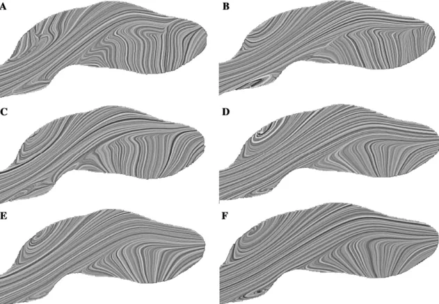
The three models with 612,000, 821,000, and 1,202,000 elements have clearly produced convergent results cerning flow pattern (Figs. 5d–5f). The generation of con-vergent planar streamline results in such a highly 3D environment is often regarded as proof of convergence for the velocity field. Therefore, it can be concluded that the minimum number of elements to obtain an accurate result in terms of the visualization of flow pattern and flow velocity is 612,000 elements (Fig. 5d).
It must be stressed that the numbers referenced here depend heavily on the underlying geometry—that is to say, on the physical dimensions of the aortic segment under investigation and on the target quantities for any particular investigation. Therefore, it is not the number of elements but the size of elements that is relevant.
Experimental Versus Numerical Flow
Comparing the experimentally generated streamlines to the numerically simulated streamlines, the run of the main
Fig. 4. Overview of the experimental setup. The closed system is shown on the left including a water tank (8), the model (5), and the pump (6). The laser is shown on the right (1) including the mirrors and prisms, which produce the fanlike split beam (4).
stream as well as the position and size of the vortices are equal (Fig. 6). The congruency of the flow pattern corrob-orates the belief that the flow volume and flow velocity are identical, but it does not imply identical pressure or shear stress.
CFD Simulation
Flow Rate
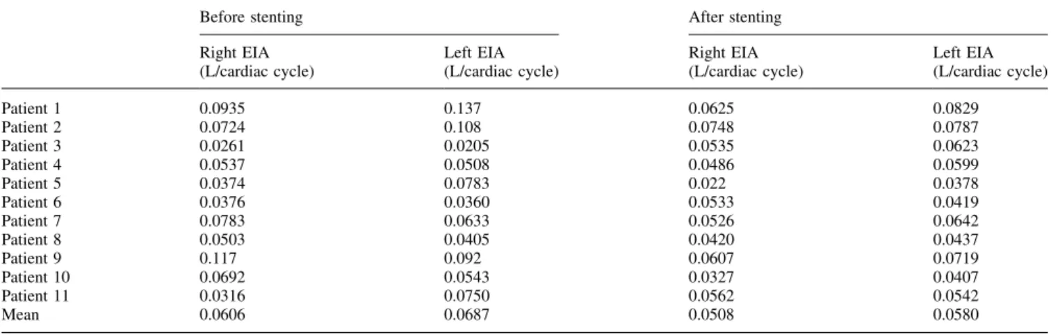
The average flow rate before and after stent-graft implan-tation was measured (Table 2). The mean flow rate before stent-graft implantation was 0.061 L per cardiac cycle for the right EIA and 0.069 L per cardiac cycle for the left EIA. After stent-graft implantation, the mean flow rate decreased to 0.051 L per cardiac cycle for the right EIA and 0.058 L pr cardiac cycle for the left EIA. The mean flow rate difference between the two legs decreased from 0.022 to 0.013 L per cardiac cycle. The EIA-ratio before and after stent-graft implantation is closer to 1 after stent-graft implantation (1-EIE-ratio: 0.29 before and 0.19 after stent-graft implanta-tion) (Table 3).
Flow Pattern
Before stent-graft implantation, the flow pattern showed areas of high velocity in the branches of the aorta and low
Fig. 5. Calculated streamlines in an identical geometric model with different number of elements: 44,000 elements (a), 103,000 elements(b), 381,000 elements (c), 612,000 elements (d), 821,000 elements (e), and 1,202,000 elements (f). Only the last three configurations (d–f) show identical flow behavior, expressing grid independency.
Fig. 6. Comparison of streamlines in a mid-sagittal plane: (a) Photo taken from the streamlines inside the silicon model; (b) the numerical calculated streamlines. The vortices as well as the mainstream are identical in position and size.
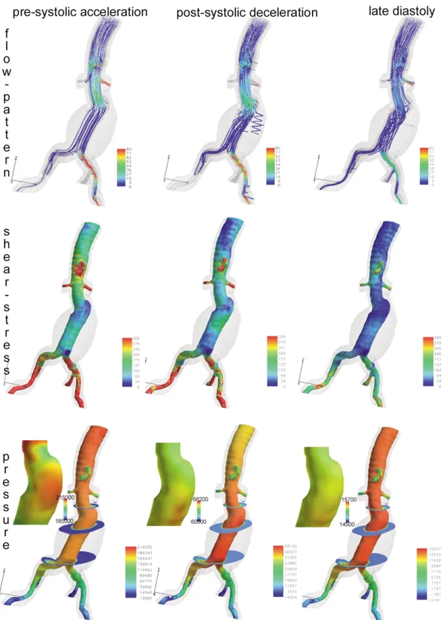
velocity in the region of the greatest diameter of the AAA, which corresponds to the normal physical findings (law of Bernoulli). Only small eddies are visible during presystolic flow acceleration (Fig. 7, flow pattern). These eddies are mostly situated outside the main stream in the concavities of the aneurysm. During the postsystolic deceleration, large vortices are visible within the aneurysm itself. During the diastole, these vortices do not fully disappear (Fig 7, flow pattern). The simulation comes to full cycle at the moment of acceleration of the flow at the beginning of the following cardiac cycle.
After stent-graft implantation, the average velocity is higher due to the smaller diameter, especially inside the stented aneurysm. No vortices are seen during presystolic acceleration (Fig. 8, flow pattern) and only small vortices appear during postsystolic deceleration (Fig. 8, flow pat-tern). At late diastoly, all vortices disappear, leading to a smooth flow pattern (Fig. 8, flow pattern). New small vor-tices appear at the distal stent end in patients with dilated common iliac arteries and might lead to endoleak type I.
Wall Pressure
Before stent-graft implantation, the areas of high wall pressure were situated where the flow was hitting the wall at a greater angle. These spots are mostly situated at the end of a vascular bend on the outer edge. On the other hand, the areas of low pressure were located at the inner edge of vascular bends (Fig 7, pressure). Inside the aneurym sac, the pressure is also elevated near the lumen, due to the fluid— structure interactions. After the systolic peak, the pressure drops significantly.
After stent-graft implantation, the maximum pressure is much lower for the aneurym sac (Fig. 8, pressure). Inside the stent, it reaches the highest value in the area of stent bifurcation. This high value is an important factor for stent migration.
At the distal end of the stent limb, near the common iliac artery bifurcation, areas of high pressure were found in the elongated vessels. These high-pressure areas were situated at the outer curvature.
The negative pressure corresponds to the Venturi effect , a special case of Bernoulli effect and is caused by the zero-force outlet condition.
Wall Shear Stress
The areas of high wall shear stress are different to the high-pressure areas. The areas of high wall shear stress are mainly situated in regions of enhanced recirculation or vortices. These locations are mostly on the inner side of kinked aneurysms. The color-coded values change rapidly over a small distance, because of the irregularity of the arteriosclerotic wall. After stent-graft implantation, there is not a significant drop in maximum shear stress. The areas
with high values are now inside the docking area. This in-creased shear stress spot is caused by a slight stenosis and wall irregularities, which is found after the intervention, due to the overlap of the stents.
Discussion
Stent-graft implantation is an attractive minimally invasive procedure to reduce the risk of rupture in AAA with well-known postoperative complications and benefits. This study investigates the effects of stent-graft implantation. The first part of the study addresses the accuracy of CFD simulations, which can be divided in two broad categories. The first category refers to grid independency, whereas the second category refers to the physical characteristics or parameters that regulate the flow.
The first part refers to the discretization of the equations that were set to describe the investigated physical phe-nomena. Numerical accuracy is directly dependent on the number of elements used for the spatial discretization of the volume of interest, as proven by the grid-independency study that was presented in the Results section. There is a threshold value concerning the required number of elements above which the simulations can be performed without lower accuracy. This threshold varies for the different he-modynamic parameters. It is higher for wall pressure and shear stress than for flow rate and flow pattern [20]. It is important to know this threshold, as computational time does not increase linearly with this value. Finer grids need more random access memory and thus require more expensive computational power. An efficient simulation technique should not only have the ability to produce results that might have clinical impact but should also be readily available to clinicians. Time is an important factor in clin-ical application. Comparing the defined threshold to other studies, it has to be pointed out that our threshold is far higher than the number of elements used in comparable studies [7, 9, 11].
In a second step, a combined experimental and compu-tational investigation of the developing blood flow field was carried out under average steady physiological flow condi-tions. The results presented here confirm a good correlation of the complex flow pattern between the numerical and experimental simulations. The positions as well as the size of the various flow characteristics such as recirculation re-gions and jets were sufficiently captured by both setups. Studies with a similar experimental environment for AAAs have already been published. These studies were also able to confirm the numerical calculation. Some of them provide additional information about flow velocity or pressure. In contrast to these studies, we used a realistic model—an approach that has so far only been used for simulations in carotic arteries or circulus Wilisii [21–25]. The use of modern CT scanning techniques, advances in the segmen-tation software, recent developments in rapid prototyping methods, and the maturing of the 3D printer permit the
construction of realistic phantom models that are well suited to fluid dynamics experiments [26, 27]. In addition, several previous studies have compared CFD simulations of bio-logical blood flow with corresponding MRI velocity map-pings [21, 22]. These studies also conclude that the results of CFD codes correspond well with the experimental investigations.
The third and main part of the study focused on the he-modynamic changes after stent-graft implantation. In terms of flow volume and flow pattern, the quantitative results of the CFD simulation after stent-graft implantation show a more equal blood flow volume through the two legs and a smoother flow pattern with a reduction in size and number of vortices. The reason for this must be the new geometry after stent-graft implantation because all other parameters remained more or less the same. The stent-graft yields a more symmetrical geometry without thinking and convexi-ties and the blood flow is almost equal due to the parallel course of the proximal part of the limbs. Li and Kleinstreuer [11] also described a reduction of vortices and a smoother flow pattern after stenting. In agreement with Chong and How [6], our results also show low flow areas inside the trunk and flow separation inside the limbs. Even if this flow
separation might be associated with thrombosis, no such thrombus was found in our population. To our knowledge no other study has described the changes in flow volume. This finding might help to explain why some patients with AAA suffer from symptoms of peripheral arteriosclerotic disease without significant stenosis. In such cases, a stent-graft implantation might be indicated even if there is only a slight risk of rupture. Focusing on the fluid–structure interaction, stent-graft implantation alone will lead to a decrease in maximum wall pressure inside the aneurysm sac. New areas of high pressure and shear stress values appear at the stent-bifurcation and to a minor degree in the docking area. Many studies have investigated the geometry of this region and its influence on stent migration.
Whereas some studies focus on stent bifurcation only, our study and that of Juchems et al. [9] point out that the docking area is also a relevant region, as it might lead to endoleak type III as a early postinterventional complication. This discrepancy is possibly caused by the fact that this region has not been specially reconstructed or displayed by the other studies. Some clinical investigations concluded that this area is the weakest and, therefore, the most vul-nerable region [28]. It has to be pointed out that in this Table 2. Flow volume (liter/cardiac cycle) through the external iliac artery before and after stent-graft implantation
Before stenting After stenting Right EIA (L/cardiac cycle) Left EIA (L/cardiac cycle) Right EIA (L/cardiac cycle) Left EIA (L/cardiac cycle) Patient 1 0.0935 0.137 0.0625 0.0829 Patient 2 0.0724 0.108 0.0748 0.0787 Patient 3 0.0261 0.0205 0.0535 0.0623 Patient 4 0.0537 0.0508 0.0486 0.0599 Patient 5 0.0374 0.0783 0.022 0.0378 Patient 6 0.0376 0.0360 0.0533 0.0419 Patient 7 0.0783 0.0633 0.0526 0.0642 Patient 8 0.0503 0.0405 0.0420 0.0437 Patient 9 0.117 0.092 0.0607 0.0719 Patient 10 0.0692 0.0543 0.0327 0.0407 Patient 11 0.0316 0.0750 0.0562 0.0542 Mean 0.0606 0.0687 0.0508 0.0580
Table 3. Flow volume ratio of the right versus the left EIA
EIA-ratio per cardiac cycle EIA-ratio per cardiac cycle
Before After Before After
Aortic stent-graft implantation Aortic stent-graft implantation
Patient 1 0.68 75 0.318 0.246 Patient 2 0.66 95 0.33 0.05 Patient 3 1.28 0.86 0.273 0.241 Patient 4 1.06 0.81 0.057 0.189 Patient 5 0.47 0.58 0.522 0.418 Patient 6 1.05 1.27 0.044 0.272 Patient 7 1.23 0.83 0.237 0.181 Patient 8 1.24 0.96 0.242 0.039 Patient 9 1.27 0.84 0.272 0.156 Patient 10 1.27 0.80 0.274 0.197 Patient 11 0.42 1.04 0.579 0.137
Fig. 7. Flow pattern, shear stress, and pressure at three different time steps in an AAA. The values for the pressure legend of the entire and zoomed figure have been adapted between the maximum values of the corresponding time step. The unit for flow is cm/sec; the unit for pressure and shear stress is Pa.
Fig. 8. Flow pattern, shear stress, and pressure at three different time steps in a stented AAA. The values for the pressure legend of the entire and zoomed figure have been adapted between the maximum values of the corresponding time step. The unit for flow is cm/sec; the unit for pressure and shear stress is Pa.
region, not the pressure as shown by Juchems et al. [9], but the shear stress plays an important role. This force is dependent on the time-step manifold being smaller than the pressure. We agree that in the early phase, this region is important until the remodelling of the stent is fulfilled. However, more important is the stent bifurcation itself. The high pressure there is one factor for stent migration. In addition, there are other factors such as stent length, greater neck angle, curvature of iliac arteries, which might lead to stent-graft migration [12, 30]. The most important factor, which interacts with the high pressure, is the enlargement of the proximal aortic neck, leading to a reduction of the radial force of the self-expanding stent [11, 30]. When this force is overcome by the traction force at the bifurcation caused by the high pressure, stent migration starts. Migration is well known in mid-term and long-term follow-up and might lead to reintervention [31–33].
Another important finding is the reduction of pressure inside the aneurysm sac, as it is the real purpose of the stent-graft implantation—shielding the aneurysm from the pul-satile blood flow. This pressure is not zero, even if the sac is completely excluded by the stent-graft. This result corre-sponds to the finding of Li and Kleinstreuer [10] and reflects the complex fluid–structure interactions between the blood flow, stent, and thrombus, which in some cases might lead to endotension [34].
A direct comparison between our results and the results of Li and Kleinstreuer [11] and Juchems et al. [9] is not possible due to the different approaches to the problem. Whereas we used deformable walls in patient-specific models, Li and Kleinstreuer [11] had idealized models and the wall in Juchems et al.’s study [9] were stiff. Another main difference is the choice of inlet and outlet param-eters, which vary among all three studies and, therefore, do not allow a comparison of the quantitative results.
Limitations
The current study has certain limitations.
1. The defined threshold for grid independency might be too low for pressure and wall shear stress. However, as long as there is a need for more computer power for realistic simulation of the environment, it is more important to visualize the hot spots and the effect of stent-graft implantation.
2. The currently available experimental setup for the first part of the study only allowed comparison of flow pattern between the experimental and numerical simulations for steady flow. It did not have the capacity to record quantitative measurements for the velocity and pressure fields. A subsequent, ongoing study is now focusing on the velocity of pulsatile flow using 3D particle tracking velocimetry [35].
3. Only the qualitative changes of wall pressure and shear stress were being investigated. The reason for this ap-proach was the lack of physiologic pressure due to the
zero-traction force at the outlet that would have given rise to false high- or low-pressure and shear stress values. 4. The results cannot be correlated to patient-specific values because the inlet parameters and wall conditions were equal for all patients.
Conclusion
After validation of the CFD program to obtain grid-inde-pendent conditions for flow volume and pattern, we were able to demonstrate quantitative and qualitative hemody-namic changes after stent-graft implantation in AAAs. The future development of more realistic models will reveal whether this new biomechanic method has the potential to help interventionalists plan and control cardiovascular interventional procedures.
References
1. Johnston KW, Rutherford RB, Tilson MD, et al. (1991) Suggested standards for reporting on arterial aneurysms. Subcommittee on Reporting Standards for Arterial Aneurysms, Ad Hoc Committee on Reporting Standards, Society for Vascular Surgery and North Ameri-can Chapter, International Society for Cardiovascular Surgery. J Vasc Surg 13:452–458
2. Alcorn HG, Wolfson SK Jr, Sutton-Tyrrell K, et al. (1996) Risk factors for abdominal aortic aneurysms in older adults enrolled in The Car-diovascular Health Study. Arterioscler Thromb Vasc Biol 16:963–970 3. Nevitt MP, Ballard DJ, Hallett JW Jr (1989) Prognosis of abdominal aortic
aneurysms. A population-based study. N Engl J Med 321:1009–1014 4. Glimaker H, Holmberg L, Elvin A, et al. (1991) Natural history of
patients with abdominal aortic aneurysm. Eur J Vasc Surg 5:125–130 5. Rydberg J, Kopecky KK, Johnson MS, et al. (2001) Endovascular re-pair of abdominal aortic aneurysms: assessment with multislice CT. Am J Roentgenol 177:607–614
6. Chong CK, How TV (2004) Flow patterns in an endovascular stent-graft for abdominal aortic aneurysm repair. J Biomech 37:89–97 7. Di Martino ES, Guadagni G, Fumero A, et al. (2001) Fluid–structure
interaction within realistic three-dimensional models of the aneurys-matic aorta as a guidance to assess the risk of rupture of the aneurysm. Med Eng Phys 23:647–655
8. Fillinger MF, Raghavan ML, Marra SP, et al. (2002) In vivo analysis of mechanical wall stress and abdominal aortic aneurysm rupture risk. J Vasc Surg 36:589–597
9. Juchems MS, Pless D, Fleiter TR, et al. (2004) [Non-invasive, multi detector row (MDR) CT based computational fluid dynamics (CFD) analysis of hemodynamics in infrarenal abdominal aortic aneurysm (AAA) before and after endovascular repair]. Rofo 176:56–61 10. Li Z, Kleinstreuer C(2005) Fluid–structure interaction effects on
sac-blood pressure and wall stress in a stented aneurysm. J Biomech Eng 127:662–671
11. Li Z, Kleinstreuer C(2005) Blood flow and structure interactions in a stented abdominal aortic aneurysm model. Med Eng Phys 27:369–382 12. Liffman K, Lawrence-Brown MM, Semmens JB, et al. (2001) Ana-lytical modeling and numerical simulation of forces in an endoluminal graft. J Endovasc Ther 8:358–371
13. Perktold K, Hofer M, Rappitsch G, et al. (1998) Validated computation of physiologic flow in a realistic coronary artery branch. J Biomech 31:217–228
14. Raghavan ML, Vorp DA, Federle MP, et al. (2000) Wall stress dis-tribution on three-dimensionally reconstructed models of human abdominal aortic aneurysm. J Vasc Surg 31:760–769
15. Walsh PW, Chin-Quee S, Moore JE Jr (2003) Flow changes in the aorta associated with the deployment of a AAA stent graft. Med Eng Phys 25:299–307
16. Wang DH, Makaroun MS, Webster MW, et al. (2002) Effect of in-traluminal thrombus on wall stress in patient-specific models of abdominal aortic aneurysm. J Vasc Surg 36:598–604
17. Kumar BV, Naidu KB (1995) Finite element analysis of nonlinear pulsatile suspension flow dynamics in blood vessels with aneurysm. Comput Biol Med 25:1–20
18. Redaelli A, Boschetti F, Inzoli F (1997) The assignment of velocity profiles in finite element simulations of pulsatile flow in arteries. Comput Biol Med 27:233–247
19. Berger SA, Goldsmith W, Lewis ER (eds.) (2000) Introduction to Bioengineering Oxford: Oxford University Press, UK
20. Moore JA, Steinman DA, Holdsworth DW, et al. (1999) Accuracy of computational hemodynamics in complex arterial geometries recon-structed from magnetic resonance imaging. Ann Biomed Eng 27:32– 41
21. Papathanasopoulou P, Zhao S, Kohler U, et al. (2003) MRI measure-ment of time-resolved wall shear stress vectors in a carotid bifurcation model, and comparison with CFD predictions. J Magn Reson Imag 17:153–162
22. Long Q, Xu XY, Bourne M, et al. (2000) Numerical study of blood flow in an anatomically realistic aorto-iliac bifurcation generated from MRI data. Magn Reson Med 43:565–576
23. Egelhoff CJ, Budwig RS, Elger DF, et al. (1999) Model studies of the flow in abdominal aortic aneurysms during resting and exercise con-ditions. J Biomech 32:1319–1329
24. Ferrandez A, David T, Bamford J, et al. (2000) Computational models of blood flow in the circle of Willis. Comput Methods Biomech Bio-med Eng 4:1–26
25. Mijovic B, Liepsch D (2003) Experimental flow studies in an elastic Y-model. Technol Health Care 11:115–141
26. Berry E, Marsden A, Dalgarno KW, et al. (2002) Flexible tubular replicas of abdominal aortic aneurysms. Proc Inst Mech Eng [H] 216:211–214
27. Knox K, Kerber CW, Singel SA, et al. (2005) Rapid prototyping to create vascular replicas from CT scan data: making tools to teach, rehearse, and choose treatment strategies. Catheter Cardiovasc Inter-vent 65:47–53
28. Kramer SC, Seifarth H, Pamler R, et al. (2001) Geometric changes in aortic endografts over a 2 year observation period. J Endovasc Ther 8:34–38
29. Mohan IV, Harris PL, Van Marrewijk CJ, et al. (2002) Factors and forces influencing stent-graft migration after endovascular aortic aneurysm repair. J Endovasc Ther 9:748–755
30. Zarins CK, Bloch DA, Crabtree T, et al. (2003) Stent graft migration after endovascular aneurysm repair: importance of proximal fixation. J Vasc Surg 38:1264–1272; discussion 1272
31. Alric P, Hinchliffe RJ, MacSweeney ST, et al. (2002) The zenith aortic stent-graft: A 5 year single-center experience. J Endovasc Ther 9:719– 728
32. Matsumura JS, Katzen BT, Hollier LH, et al. (2001) Update on the bifurcated EXCLUDER endoprosthesis: phase I results. J Vasc Surg 33:S150–S153
33. Ohki T, Veith FJ, Shaw P, et al. (2001) Increasing incidence of mid-term and long-mid-term complications after endovascular graft repair of abdominal aortic aneurysms: A note of caution based on a 9-year experience. Ann Surg 234:323–334; discussion 334–325
34. White GH, May J, Petrasek P, et al. (1999) Endotension: An expla-nation for continued AAA growth after successful endoluminal repair. J Endovasc Surg 6:308–315
35. Willneff J (2002) 3D particle tracking velocimentry based on image and object space information. In:ISPRS Commission V Symposium, International Archives of Photography, Remote Sensing and Informa-tion Sience. Corfu, Greece, 2002, Part 5