Design of interactive maps for ocean dynamics data

Design of Interactive Maps

for Ocean Dynamics Data

by

Mohamad Mirhi

B.E., American University of Beirut (2011)

S.M., Massachusetts Institute of Technology (2013)

Submitted to the Department of Mechanical Engineering

in partial fulfillment of the requirements for the degree of

Mechanical Engineer

at the

MASSACHUSETTS INSTITUTE OF TECHNOLOGY

February 2019

Massachusetts Institute of Technology 2019. All rights reserved.

Author...

Certified by...

Accepted by ...

FEB 25 2019

LIBRARIES

Signature redacted

D1tartme

neering

19 September 2018

Signature redacted

Pierre Lermusiaux

Professo

sociate Department Head for Operations

S.-ervisor

Signature

rUactWd

Nicolas IAadjiconstantinoP

Chairman, Committee on Graduate Students

Design of Interactive Maps

for Ocean Dynamics Data

by

Mohamad Mirhi

Submitted to the Department of Mechanical Engineering on 19 September 2018, in partial fulfillment of the

requirements for the degree of Mechanical Engineer

Abstract

Comprehensive spatiotemporal modeling and forecasting systems for ocean dynamics necessitate robust and efficient data delivery and visualization techniques. The multi-disciplinary simulation, estimation, and assimilation systems group at MIT (MSEAS) focuses on capturing and predicting diverse ocean dynamics, including physics, acous-tics, and biology on varied scales, thereby developing new methods for multi-resolution ocean prediction and analysis, including data generation and assimilation. The group has primarily used non-interactive ocean plots to visualize its simulated and mea-sured data. Although these maps and sections allow for analysis of ocean physics and the underlying numerical schemes, more interactive maps provide more user control over depicted data, allowing easier study and pattern identification on multiple scales. Integrating static and geospatial data in dynamic visualization creates a heightened viewpoint for analysis, enhances ocean monitoring and prediction, and contributes to building scientific knowledge. This thesis focuses on explaining the motivation behind and the methodologies applied in designing these interactive maps.

Thesis Supervisor: Pierre Lermusiaux

Acknowledgments

First, I would like to express my deep gratitude to Professor Pierre Lermusiaux. Since he gave me the opportunity to join his MSEAS group, he offered nothing but patient guidance and useful advice towards the completion of the thesis. My grateful thanks are also extended to the members of the MSEAS group especially to Deepak Subramani, Corbin Foucart, Chris Mirabito and Wael H. Ali who welcomed me to the group and significantly contributed to the work. I would also like to extend my thanks to some amazing MIT people, who supported me over the years, namely Leslie Regan, Jason McKnight, Dean Staton, Prof Abeyaratne, Prof Karnik and Prof Hardt.

Second, I am blessed with an extraordinary group of people who have been and will always be there for me. Mike has been my main support in times of stress. Bardan has always rooted for me. Many thanks to Adham, Fadel, Ozzy, Assil, Dahlia, Taha, Leila, Khaled, Hens, 1-95 and others.

Finally, I wish to thank my family for their support and encouragement throughout my studies. Thank you Salwa, Hussein, Qasim and Rana, Samer and Miriam, Sahar, and my three beautiful nieces, Reine, Rayan and Krystel.

*The MSEAS group is also grateful to the Office of Naval Research for support un-der Grants N00014-14-1-0725 (Bays-DA), N00014-14-1-0476 (Science of Autonomy

LEARNS) and N00014-15-1-2616 (DRI-NASCar), to the National Science

Founda-tion for support under grant EAR-1520825 (Hazards SEES - ALPHA), and to the Defense Advanced Research Projects Agency for support under Grant N66001-16-C-4003 (POSYDON-POINT), each to the Massachusetts Institute of Technology (MIT). We also thank the MIT Tata Center for their student support during the years

Contents

1 Motivation and Thesis Outline 8

1.1 Motivation . . . . 8

1.2 Thesis Outline. . . . . 9

2 Background 13 2.1 Oceans Keep Us Alive . . . . 13

2.2 The Significance of Ocean Data . . . . 14

2.2.1 Climate and Weather . . . . 15

2.2.2 Carbon Sequestration . . . . 16

2.2.3 Resources . . . . 17

2.2.4 Economy and Society . . . . 18

3 MSEAS Ocean Data Visualization 25 3.1 MSEAS . . . ... . . . ... . . . . 25

3.2 MSEAS Data Cycle. . . . . 26

3.2.1 Data Discovery . . . . 26

3.2.2 Data Visualization . . . . 28

3.2.3 Web Experience. . . . . 30

4 Map Design and Implementation 38 4.1 The Wishlist . . . . 38

4.2 The Options . . . . 39

4.2.1 Option 1 . . . . 40

4.2.2 Option 2 . . . . 40

4.2.4 Option 4 . . . . 4.3 The New Interactive Visualization Code 4.4 The Map

4.4.1 The Map Variable 4.4.2 Baselayer Map . 4.4.3 Data Layers . . . 4.4.4 Control Panel . . 4.4.5 Sliders . . . . 4.4.6 Other elements 4.4.7 Cache Function The Web Structure . . . The Mobile Device . . . The Applications . . . . The Demo . . . .

5 Conclusion and Future Work 5.1 Conclusion . . . . 5.2 Future Work . . . . . . . . 41 . . . . 42 4.5 4.6 4.7 4.8 . . . . . . . . . . . . . . . . . . . . . . . . . . . . . . . . . . . . . . . . . . . . . . . . . . . . . . . . 42 43 44 44 49 50 51 52 52 54 55 58 60 60 61

List of Figures

2-1 Ocean Zones . . . .. . . . . 14

2-2 Ocean Carbon Cycle . . . . 17

2-3 Marine Energy Technologies . . . . 19

3-1 Ocean Dynamics Examples - top left: vorticity profile (NSF-ALPHA 2017), top right: Backward FTLE profile (NSF-ALPHA 2017), bot-tom left: standard deviation of sound speed field (POSYDON-POINT 2018), bottom right: temperature profile (POSYDON-POINT 2018) . 30 3-2 Sea Exercises . . . . 31

3-3 POSYDON-POINT Calendar . . . . 32

3-4 Domain and Depth . . . . 33

3-5 Data Variable . . . . 34

3-6 Time Thumbnails . . . . 35

3-7 Desired Temperature Field . . . . 36

4-1 The Map View: a schematic of a generated map that shows a temper-ature field and a snapshot of the animated velocity field around the Martha's Vineyard and Nantucket's coastal region; part of the NSF-ALPHA MSEAS sea exercise issued on August 6th, 2018 . . . . 43

4-2 2018 NSF-ALPHA Data Layer Snapshots - (1: Temperature field over-laid with velocity direction field in full domain at 0 m, 2: salinity field overlaid with animated velocity in full domain at 0 m, 3: vorticity field in full domain at 0 m, 4: velocity vector field (magnitude and direc-tion) in full domain at 0 m, 5: standard deviation field of the seawater density in zoomed-in domain at a depth of 20 m, 6: standard devia-tion field of temperature overlaid with mean animated velocity field in zoomed-in domain at a depth of 20 in). Note that the fields of 1,2,3, and 4 have a 600 m resolution, while those of 5 and 6 have a 200 in

resolution . . . . 4-3 POSYDON-POINT Data Layer Snapshots - (1: temperature field over-laid with animated velocity in full domain at 0 m, 2: sound speed field in full domain at 0 m, 3: barotropic velocity vector field (magnitude and direction) in full domain at 0 m, 4: temperature field overlaid with animated velocity in full domain at a depth of 500 in, sound speed field in full domain at a depth of 500 in). Note that all these fields have a resolution of 3 km. . . . . Sample ASCII File Format (taken from a salinity field)

Data Rendering of a Scalar Field . . . . Popup Function Example (salinity field) . . . . Salinity Colorbar Example . . . . Example Control Panels - 1: an ocean physics map, 2: certainty m ap . . . . Depth and Time Range Sliders . . . . Input File Parameters . . . . New Web Front End . . . . Mobile Device Map Views (left: landscape mode, right: NSF-ALPHA LCS 6 hour Backward FTLE Map . . . .

POSYDON-POINT Sound Speed Field Maps . . . . .

an ocean un-portrait mode) 45 46 47 48 48 49 50 51 53 54 55 56 57 4-4 4-5 4-6 4-7 4-8 4-9 4-10 4-11 4-12 4-13 4-14

Chapter 1

Motivation and Thesis Outline

1.1

Motivation

Data delivery and visualization software for ocean dynamics serves numerous pur-poses. They are tools by which ocean monitoring and forecasting products are dis-tributed to end-users. These ocean products have a major impact on industries such as fisheries, coastal management, shipping, transport, marine recreation, maritime surveillance, and security [11 [2] [3]. Ocean data visualization software also depicts the chemical characteristics and quality of water in certain areas. They also help identify the potential for seabed mining and resource retention as the resources on the land are increasingly depleted. They can provide insights into the organic re-lationship between the biogeochemistry of the ocean and the weather and climate. Biological functioning modulates certain gases in the atmosphere, which influences its climate [4]. _{This influence is manifested in certain physical and biological}

pro-cesses that change in space and time and are often simulated using ocean observing and modeling systems. Moreover, ocean data provides the basis for innovative moni-toring and mitigation of issues such as water pollution, oil spills, and loss of marine productivity [5] [61 [71 [81. All these benefits also essentially drive scientific knowledge.

Although data collection/generation is the first step towards answering relevant questions, effective communication of data through visualization techniques renders

complex multivariate data much more accessible. The MSEAS group at MIT gener-ates different data variables using novel methods of multi-scale modeling and uncer-tainty quantification [9] [10] [111. This data is often encoded in visual objects such as graphs, contour plots, or static maps (horizontal maps, cross-sections, etc.) [121 [131 [141. Although these tools convey ideas effectively, interactive maps that serve user-specific purposes would provide more insight into such complex multi-resolution ocean data.

Since most of the generated data varies with time and space, dynamic maps have the advantage of capturing change in a very intuitive way. In addition to clearly com-municating information, they stimulate user engagement by giving them the ability to control what they want to see and how they want to see it. For example, one could examine the time change of temperature in a certain ocean area using the features of one dynamic map that is fully interactive and allows multi-resolution views, as opposed to several static maps, each corresponding to a certain time of the day.

This thesis builds upon the power of interactive maps. It also sets up and builds the tools required for developing dynamic maps for ocean physics and uncertainty data generated in MSEAS, using and expanding upon existing open-source software.

1.2

Thesis Outline

Chapter 2 is a background review of the indispensable impact of oceans on the life on Earth. It highlights the organic relationship between ocean-related processes and other necessary phenomena of life such as moderation of weather and climate, en-suring biodiversity and symbiotic habitats, providing resources and raw materials, and mitigating global warming. It also explains the importance of studying oceans and data that characterize ocean physics, focusing on certain economic sectors and applications that could make the best use of such data.

power is incomplete without effective communication of the data using good practices of data visualization. It describes the multi-scale equations and the uncertainty quan-tification models developed by the MSEAS group at MIT. It then depicts the need for interactive multilayered maps and compares their experience to more traditional infographics used by the MSEAS group such as snapshot images and static webpages.

Chapter 4 describes, in detail, the engineering process adopted in building the maps. This includes the educated selection of software, libraries, and plugins, and the placement of the maps within the MSEAS portal. Demonstrating examples of maps included in some MSEAS projects are also included.

Chapter 5 concludes the thesis and gives a brief insight into possible future en-hancements of the methods, product and applications.

Bibliography

[1] P. F. J Lermusiaux, P. J. Haley, Jr, and N. K. Yilmaz. Environmental prediction, path planning and adaptive sampling: sensing and modeling for efficient ocean monitoring, management and pollution control. Sea Technology, 48(9):35-38,

2007.

[2] P. F. J. Lermusiaux, T. Lolla, P. J. Haley, Jr., K. Yigit, M. P. Ueckermann, T. Sondergaard, and W. G. Leslie. Science of autonomy: Time-optimal path planning and adaptive sampling for swarms of ocean vehicles. In Tom Curtin, editor, Springer Handbook of Ocean Engineering: Autonomous Ocean Vehicles,

Subsystems and Control, chapter 21, pages 481-498. Springer, 2016.

[31 P. F. J. Lermusiaux, D. N. Subramani, J. Lin, C. S. Kulkarni, A. Gupta, A. Dutt,

T. Lolla, P. J. Haley, Jr., W. H. Ali, C. Mirabito, and S. Jana. A future for intelligent autonomous ocean observing systems. Journal of Marine Research,

75(6):765-813, November 2017. The Sea. Volume 17, The Science of Ocean

Prediction, Part 2.

[41 Lynn Margulis and J.e. Lovelock. Biological modulation of the earth's atmo-sphere. Icarus, 21(4):471-489, 1974.

[5] Pierre Lermusiaux, Patrick Haley, Wayne Leslie, Arpit Agarwal, Oleg Logutov, and Lisa Burton. Multiscale physical and biological dynamics in the philippine archipelago: Predictions and processes. Oceanography, 24(01):70-89, Jan 2011. [61 Michela De Dominicis, Silvia Falchetti, Francesco Trotta, Nadia Pinardi, Luca

Giacomelli, Ernesto Napolitano, Leopoldo Fazioli, Roberto Sorgente, Patrick J. Haley, Jr., Pierre F. J. Lermusiaux, F. Martins, and M. Cocco. A relocat-able ocean model in support of environmental emergencies. Ocean Dynamics,

64(5):667-688, 2014.

[7J C. S. Kulkarni, P. J. Haley, Jr., P. F. J. Lermusiaux, A. Dutt, A. Gupta,

C. Mirabito, D. N. Subramani, S. Jana, W. H. Ali, T. Peacock, C. M. Royo,

A. Rzeznik, and R. Supekar. Real-time sediment plume modeling in the South-ern California Bight. In OCEANS Conference 2018, Charleston, SC, October

[8] J. Coulin, P. J. Haley, Jr., S. Jana, C. S. Kulkarni, P. F. J. Lermusiaux, and T. Peacock. Environmental ocean and plume modeling for deep sea mining in the bismarck sea. In Oceans 2017 - Anchorage, Anchorage, AK, September 2017.

[9] Patrick J. Haley, Jr. and Pierre F. J. Lermusiaux. Multiscale two-way embedding schemes for free-surface primitive equations in the "Multidisciplinary Simulation, Estimation and Assimilation System". Ocean Dynamics, 60(6):1497-1537, De-cember 2010.

[101 P. J. Haley, Jr., A. Agarwal, and P. F. J. Lermusiaux. Optimizing velocities and transports for complex coastal regions and archipelagos. Ocean Modeling,

89:1-28, 2015.

[11] P. F. J. Lermusiaux, C.-S. Chiu, G. G. Gawarkiewicz, P. Abbot, A. R.

Robin-son, R. N. Miller, P. J. Haley, Jr, W. G. Leslie, S. J. Majumdar, A. Pang, and F. Lekien. Quantifying uncertainties in ocean predictions. Oceanography, 19(1):92-105, 2006.

[121 Suzana Djurcilov, Kwansik Kim, Pierre F. J. Lermusiaux, and Alex Pang. Vol-ume rendering data with uncertainty information. In David S. Ebert, Jean M. Favre, and Ronald Peikert, editors, Data Visualization 2001, Joint Eurographics

- IEEE TCVG Symposium on Visualization, pages 243-252, 355-356. Springer Vienna, 2001.

[13] Suzana Djurcilov, Kwansik Kim, Pierre Lermusiaux, and Alex Pang. Visualizing scalar volumetric data with uncertainty. Computers and Graphics,

26(2):239-248, 2002.

[141 Arkopal Dutt, Deepak N. Subramani, Chinmay S. Kulkarni, and Pierre F. J. Lermusiaux. Clustering of massive ensemble of vehicle trajectories in strong, dynamic and uncertain ocean flows. In OCEANS Conference 2018, Charleston,

Chapter 2

Background

2.1

Oceans Keep Us Alive

Oceans cover 71% of Earth's surface I1l and contain 97% of the water available on the

planet [2]. They have been always recognized as one of the most important natural

resources. Their diverse habitats and ecological systems host 99% of the living space

on Earth [3]. In oceans, life stretches from the epipelagic surfaces -

where enough

sun-light penetrates for photosynthesis [4]

-

to extreme environments in the hadal zone,

tens of thousands of feet below the surface. Figure 2-1 depicts the different ocean

zones.

Figure 2-1: Ocean Zones [5]

The profound value of oceans is not only ecological but also extends to economic

and social impact [3]. However, in order to better understand how oceans affect us,

optimize the sustainable use of their resources and act on hazardous trends, it is

crucial to measure, model and visualize ocean data.

In his opening remarks to the Ocean Conference (Sweden and Fiji, June 2017), the

UN Secretary General Antonio Guterres called for a coordinated international effort

to mitigate the intensity of the threat on oceans given the rising sea levels, climate

change, pollution and overfishing. His global action list emphasized that we must

deepen our knowledge base, with better data, information and analysis because we

simply cannot improve what we do not measure. [6]

2.2

The Significance of Ocean Data

In this chapter, we discuss some of the biological, physical, economic and social

interactions that necessitate the study of ocean dynamics.

2.2.1

Climate and Weather

Oceans regulate Earth's climate and define its different weather zones, which makes this planet habitable. Without oceans, weather zones would be more extreme [7J. Therefore, understanding ocean physics is extremely important especially amid the increasing risks of climate change and the accompanying disasters such as hurricanes, floods, droughts, heat waves, and melting glaciers. Not only do oceans store the ma-jority of solar radiation but also contribute to the even distribution of heat around the globe.

First, oceans are a major player in the hydrological cycle on Earth [8]. Solar heat causes water at the surface of the ocean to evaporate. Water vapor then rises and condenses as clouds that are driven by trade winds and cause rain and storms else-where on land. Therefore, oceans facilitate the continuous movement of water. The deep understanding of the ocean's properties translates into more control over this cycle that is a guarantee for life for many species.

Second, oceans facilitate the thermohaline circulation by distributing heat and salt around the globe [1]. Two forces mainly drive ocean circulation. These are wind stress - manifested by surface winds due to Ekman spirals - and buoyancy flux be-tween atmosphere and ocean [9] - controlled by temperature and salinity gradients and the subsequent density stratification. Although wind-driven forces seem to be more vigorous than buoyancy in regulating the redistribution of salt and heat in the upper kilometers, buoyancy effect is full-depth and often involves ocean overturning that translates into a direct effect on climate [10]. Ocean currents that often trace the coastlines, act as massive heat belts that moderate global climate by carrying heat from one zone to another. For instance, they can transport warm water and precipitation from the equator towards the poles and cold water from the poles back to the tropics [11].

Third, vertical motions in the ocean are critical to the exchange of heat and gases such as CO2 between the surface layer and the deep ocean. Processes such as

upwelling take place in the ocean. Dense, cooler, more nutrient-rich water travels up from the deep ocean to replace the warmer, nutrient-depleted surface water [121. This phenomenon is crucial for many biological processes that conserve several marine ecosystems.

The study and visualization of ocean data in a way that demonstrates trends in parameters such as temperature, salinity and stress largely contribute to better under-standing of the described cycles and more effective mitigation of potential calamities.

2.2.2

Carbon Sequestration

Oceans play a key role in the carbon cycle as they take up a large percentage of at-mospheric CO2 [131. Carbon dioxide hydrates are an effective vehicle for deep ocean

carbon sequestration [14]. These hydrates are typically denser than seawater, so they naturally sink to the deep ocean while dissolving, which facilitate dispersion.

Burning fossil fuels has accumulated carbon dioxide in the atmosphere, which exacerbates the greenhouse effect. Oceans have always captured a part of the at-mospheric carbon. However, this cycle is not infinite. One NASA model has shown that doubling the level of pre-industrial CO2 increases the ocean's carbon content, but as water temperature increases, its ability to dissolve CO₂ drops [151. This drop accumulates more CO2 in the atmosphere, which causes a rise in temperature.

The global oceans are connected by deep currents and surface currents. Carbon from the atmosphere enters the ocean depths in areas of deep water formation in the North Atlantic and offshore of the Antarctic Peninsula. Where deep currents rise towards the surface, they can release carbon dioxide stored centuries ago [16]. This is shown in Figure 2-2

oarbons

Depth (m)

>0(X 4000 0

Figure 2-2: Ocean Carbon Cycle [16]

In addition to deep injection, priming the biological pump by iron fertilization of the ocean is another approach to sequester carbon. Iron stimulates the production of phytoplanktons, which leads to an algal bloom that nourishes sea organisms and eventually accelerates CO2 dissolving [17].

Therefore, it is important to characterize seawater properties and model its tem-perature, salinity and alkalinity in order to quantify the water's ability to dissolve

CO2 and mitigate global warming.

2.2.3

Resources

Oceans are a large source of a number of human necessities. This includes - but is not limited to- food, oil and gas, energy, salt, sand, gravel, minerals and other com-mercially important materials such as diamond, manganese, copper and nickel [18].

It has become apparent that seabed mining carries a lot of potential to supply dwindling resources needed by humans. With this discovery, a number of questions about the impact of deep-sea mining arose, especially related to its effect on the ocean's ecosystems and the circulation of deep ocean pollutants [19]. Deep sea-mining

activities are being largely studied and it is unequivocally important to model ocean

dynamics during these studies.[20]

In one of the MSEAS activities, namely plume modeling for deep sea mining in

the Bismarck sea[19], the MSEAS relied on a number of models to carry out the

experiment. The modeling capabilities included implicit two-way nesting for

multi-scale hydrostatic primitive equation (PE) dynamics with a nonlinear free-surface

and a high-order finite element code on unstructured grids for non-hydrostatic

pro-cesses [21] [22] [231 [24]. Additional subsystems included Lagrangian Coherent

Struc-tures, non-Gaussian data assimilation and adaptive sampling.

2.2.4

Economy and Society

Currently, 40% of the world's population inhabits coastal regions (United Nations,

2015) and and over 3 billion people depend directly on marine resources for livelihoods

and welfare [25]. The services provided by the oceanic ecological systems contribute

significantly to welfare and therefore represent a big portion of the economic value

of the planet

[3].

Coastal environments, including estuaries, coastal wetlands, beds

of sea grass and algae, coral reefs, and continental shelves cover only 6.3% of the

world's surface, but are responsible for 43% of the estimated value of the world's

ecosystem services [26]. Preserving this economic value is crucially important to

alle-viate poverty and provide job opportunities. Sustainable governance of these systems

necessitate accurate modeling of coastal oceanic regions. In fact, the coastal ocean is

a prime example of multi-scale nonlinear fluid dynamics [25].

The economic value of the oceans is inextricably linked to social welfare. The

social importance of the oceans for global transportation and as a unifying element

in the cultures of many coastal countries cannot be overstated [3].

a. Fisheries

Modeling and visualizing ocean physics by fisheries are necessary tools for

op-timal management of fisheries and sustainable seafood supply. Overfishing has

been one of the most problematic issues oceans face as it depletes the adult fish

population in some regions [27]. Approximately 57% of fish stocks are

fully-exploited and 30% over-fully-exploited, depleted or recovering [28].

Multi-scale modeling of coastal oceans involves study of ocean fields and their

uncertainties and coastal ecosystem-based scenario analyses that help fisheries

make better technical decisions about their fishing methods and the frequency

they fish at. In addition, ocean data helps design more complex systems that

optimize guidance sensors for boats. It also helps understand changes in the

characteristic quality of fishes in terms of their plasma chloride levels and muscle

tissue moisture.

b. Energy

A number of marine renewable energy technologies have tested to be promising

(shown in Figure 2-3). Although these technologies are at their early stage of

development, they are expected to grow. Globally, the renewable energy sector

between 2004 and 2013, increased from 85 to 560 GW (led by the wind

indus-try) [29].

Ocean Energy

5 ftchnologies creating

re-ewabe e Veg from seas and oceans

With the urgency of providing a sustainable future for the Earth, ocean energy

sources prove to be necessary. As solar radiation is converted to wind energy

and later wave energy, the amount of energy per unit volume becomes more

concentrated [31]. Therefore, considering that waves are an intensified form of

wind energy that is capable to travel long distances with minimal losses, the

wave energy sector is expected to grow till it equals the importance of offshore

wind energy.

The ocean hosts a number of energy extraction options [32]. Examples include

(1) wave energy technologies that use of ocean swells created by persistent

winds [29], (2) tidal energy technologies that garner the energy effect of the

pull between the moon and the sun in the motion of tides, (3) current energy

systems that capture the enormous amount of energy contained in ocean

cur-rents, thanks to the water density, (4) salinity gradient systems such as reverse

electrodialysis and pressure retarded osmosis, and (5) thermal gradient systems

that run a heat engine between shallow and deep ocean levels.

The study and development of the potential of these energy sources necessitate

the knowledge of the temporal and spatial variations of the ocean physics.

c. Maritime Security and Surveillance

The development of comprehensive and real-time systems, targeted towards

surveillance and security in marine regions, requires advanced accurate

multi-scale ocean modeling. For instance, geospatial sound speed models are

ex-tremely helpful in detection of underwater objects and contribute to long-range

low-frequency acoustical research [33] [341 [35].

d. Other sectors

Other sectors that largely rely on ocean data include tourism (in which

tem-perature, salinity and ocean current profiles impact the type of recreational

activities to be established), shipping, coastal management serviced to protect

against flood and erosion, hazard prediction analyses, and development of ad-vanced systems such as underwater navigation and autonomous vehicles.

Hence, ocean dynamics data are undeniably crucial for the betterment of science, economies, and societies in general.

Bibliography

[11 Stefan Rahmstorf. Ocean circulation and climate during the past 120,000 years.

Nature, 419(6903):207-214, Dec 2002.

[21 NOAA. Where is all of the earth's water?:

https://oceanservice.noaa.gov/facts/wherewater.html. NOAA 's National Ocean Service, Dec 2009.

[3] Robert Costanza. The ecological, economic, and social importance of the oceans.

Ecological Economics, 31(2):199-213, 1999.

[4] Weimin Gao, Xu Shi, Jieying Wu, Yuguang Jin, Weiwen Zhang, and Deirdre R. Meldrum. Phylogenetic and gene expression analysis of cyanobacteria and di-atoms in the twilight waters of the temperate northeast pacific ocean.

Springer-Link, Jun 2011.

[5] J.D. Knight. Layers of the ocean - deep sea creatures on sea and sky: http://www.seasky.org/deep-sea/ocean-layers.html.

[61 United Nations. Secretary-general's opening remarks to the ocean conference (sweden and fiji), 2017: https://www.un.org/sg/en/content/sg/statement/2017-06-05/secretary-generals-opening-remarks-ocean-conference-delivered.

[7] NOAA. How does the ocean affect climate and weather on land?: https://oceanexplorer.noaa.gov/facts/climate.html. Deepwater Exploration of

the Marianas RSS, Jun 2013.

[81 Moustafa T. Chahine. The hydrological cycle and its influence on climate. Nature,

359(6394):373-380, 1992.

[9] M.f. Cronin and J. Sprintall. Wind and buoyancy-forced upper ocean.

Encyclo-pedia of Ocean Sciences, page 3219-3226, 2001.

[10] Andrew Revkin. Global Warming: Understanding the Forecast. Abbeville Press,

1992.

[111 Wallace Broeker. The great ocean conveyor. Oceanography, 4(2):79-89, 1991. [12] T Sarhan. Upwelling mechanisms in the northwestern alboran sea. Journal of

[13] Roger Revelle and Hans E. Suess. Carbon dioxide exchange between atmosphere and ocean and the question of an increase of atmospheric co2 during the past decades. Tellus, 9(1):18-27, 1957.

[141 Olivia R. West, Costas Tsouris, Sangyong Lee, Scott D. Mccallum, and Liyuan Liang. Negatively buoyant co2-hydrate composite for ocean carbon sequestration.

AIChE Journal, 49(1):283-285, 2003.

[151 J. G. Canadell, C. Le Quere, M. R. Raupach, C. B. Field, E. T. Buitenhuis,

P. Ciais, T. J. Conway, N. P. Gillett, R. A. Houghton, G. Marland, and et al. Contributions to accelerating atmospheric co2 growth from economic activity, carbon intensity, and efficiency of natural sinks. Proceedings of the National

Academy of Sciences, 104(47):18866-18870, 2007.

[16] NASA. The carbon cycle: : https://earthobservatory.nasa.gov/features/carboncycle. [171 K H Coale, K S Johnson, S E Fitzwater, R M Gordon, S Tanner, F P Chavez,

L Ferioli, C Sakamoto, P Rogers, F Millero, and et al. A massive phytoplank-ton bloom induced by an ecosystem-scale iron fertilization experiment in the equatorial pacific ocean. Nature., Oct 1996.

[18] P. A. Rona. Geology: Resources of the sea floor. Science, 299(5607):673-674,

2003.

[19] J. Coulin, P. J. Haley, Jr., S. Jana, C. S. Kulkarni, P. F. J. Lermusiaux, and

T. Peacock. Environmental ocean and plume modeling for deep sea mining in the bismarck sea. In Oceans 2017 - Anchorage, Anchorage, AK, September 2017.

[201 C. S. Kulkarni, P. J. Haley, Jr., P. F. J. Lermusiaux, A. Dutt, A. Gupta,

C. Mirabito, D. N. Subramani, S. Jana, W. H. Ali, T. Peacock, C. M. Royo,

A. Rzeznik, and R. Supekar. Real-time sediment plume modeling in the South-ern California Bight. In OCEANS Conference 2018, Charleston, SC, October

2018. IEEE. In press.

[21] Patrick J. Haley, Jr. and Pierre F. J. Lermusiaux. Multiscale two-way embedding schemes for free-surface primitive equations in the "Multidisciplinary Simulation, Estimation and Assimilation System". Ocean Dynamics, 60(6):1497-1537, De-cember 2010.

[22] P. J. Haley, Jr., A. Agarwal, and P. F. J. Lermusiaux. Optimizing velocities and transports for complex coastal regions and archipelagos. Ocean Modeling,

89:1-28, 2015.

[231 M. P. Ueckermann and P. F. J. Lermusiaux. Hybridizable discontinuous Galerkin projection methods for Navier-Stokes and Boussinesq equations. Journal of

[24] C. Foucart, C. Mirabito, P. J. Haley, Jr., and P. F. J. Lermusiaux. Distributed implementation and verification of hybridizable discontinuous Galerkin methods for nonhydrostatic ocean processes. In OCEANS Conference 2018, Charleston,

SC, October 2018. IEEE. In press.

[25] Deepak Narayanan Subramani. Probabilistic regional ocean predictions:

stochas-tic fields and optimal planning. 2018.

[26] Mostafa Kamal Tolba. Our fragile world: challenges and opportunities for

sus-tainable development. Eolss, 2001.

[271 E. S. Russell. Some theoretical considerations on the "overfishing" problem. ICES

Journal of Marine Science, 6(1):3-20, 1931.

[28] David J. Attard, Malgosia Fitzmaurice, and Alexandros X. M. Ntovas. The IMLI treatise on global ocean governance: UN specialized agencies and global

ocean governance Volume II. Oxford University Press, 2018.

[29] Eugen Rusu and Florin Onea. A review of the technologies for wave energy extraction. Clean Energy, 2(1):10-19, Jul 2018.

[30] EnergyWall. Ocean energy: http://energywall.in/ocean-energy. Mar 2018. [31] Australian Academy of Science. Harnessing the power of the ocean:

https://www.science.org.au/curious/technology-future/ocean-power. Sep 2017.

[32] S. Deluca, S. Zanforlin, B. Rocchio, P. J. Haley, C. Foucart, C. Mirabito, and

P. F. J. Lermusiaux. Scalable coupled ocean and water turbine modeling for assessing ocean energy extraction. In OCEANS Conference 2018, Charleston,

SC, October 2018. IEEE. In press.

[33] A. R. Robinson and P. F. J. Lermusiaux. Prediction systems with data assimi-lation for coupled ocean science and ocean acoustics. In A. Tolstoy et al, editor,

Proceedings of the Sixth International Conference on Theoretical and Compu-tational Acoustics, pages 325-342. World Scientific Publishing, 2004. Refereed

invited Keynote Manuscript.

[34] Pierre F. J. Lermusiaux, Jinshan Xu, Chi-Fang Chen, Sen Jan, L.Y. Chiu, and Yiing-Jang Yang. Coupled ocean-acoustic prediction of transmission loss in a continental shelfbreak region: Predictive skill, uncertainty quantification, and dynamical sensitivities. IEEE Journal of Oceanic Engineering, 35(4):895-916, October 2010.

[35] Frans-Peter A. Lam, Patrick J. Haley, Jr., Jeroen Janmaat, Pierre F. J. Ler-musiaux, Wayne G. Leslie, Mathijs W. Schouten, Lianke A. te Raa, and Michel Rixen. At-sea real-time coupled four-dimensional oceanographic and acoustic forecasts during Battlespace Preparation 2007. Journal of Marine Systems,

Chapter 3

MSEAS Ocean Data Visualization

The development of appropriate data visualization tools must be based upon deep understanding of the nature of the data, the relationship among different data sets, the desired features, and the user expectations. The design of our ocean dynamics maps is based upon the models developed by the Multidisciplinary Simulation, Estimation, and Assimilation Systems (MSEAS) group at MIT. In this chapter, we start from the research activities and visualization tools of MSEAS and expand to data visualization features that reflect an enhancement of the current tools.

3.1

MSEAS

MSEAS is a research group, focused on regional ocean data assimilation and led by Professor Pierre Lermusiaux. The group creates and utilizes new methods for multi-scale modeling, uncertainty quantification, data assimilation and the guidance of autonomous vehicles. These advances are then utilized to better understand phys-ical, acoustical and biological interactions [11.

The group hosts an extensive list of ocean-related research projects and adopts an integrated approach to characterize complex fluid systems and develop compu-tational models for prediction and quantification of ocean dynamics. The group is also involved in several sea exercises that test and validate the theory. Machine

learning techniques are then applied to enhance the theoretical models. Within data assimilation, a number of techniques are applied. Examples include direct multi-scale filtering and smoothing, multi-resolution data assimilation and scale-decomposition, and multi-scale adaptive sampling and modeling.

3.2

MSEAS Data Cycle

3.2.1

Data Discovery

Any data cycle starts with mining the data and understanding a potential strategy for a story. Data mining involves numerical computation or experimental results. The MSEAS group has mastered the data discovery applications starting from their PE model, described below.

PE Model

The MSEAS group utilizes their stochastic ocean PE model that mainly solves a set of nonlinear high-order partial differential equations called Primitive Equations (PE) [2]. Primitive equations are typically conservation equations of mass, momentum and thermal energy. These equations are constrained by a set of initial conditions, boundary conditions, and forcing parameters. The model output consists of a set of prognostic variables that are governed by time evolution equations, and diagnostic variables that are non-prognostic. In order to test and validate the PE model, MSEAS also works with real ocean data because data motivates discoveries and fosters new fundamental ideas.

Data Fields

In the context of map design, it is important to understand the nature of the forecasted ocean dynamics. The data variables intended to visualize are:

These are the fields that vary spatiotemporally and are a result of numerical solutions of the PE model. These data fields are divided among:

1. Scalar Fields

These fields are parameter distributions in space, whose values at each point - defined by an intersection of a latitude line, longitude line and a depth level- are scalar quantities. Examples include:

- Temperature: Temperature is a prognostic variable, computed using the first law of thermodynamics [after solving Navier-Stoke's (balance of momentum) equation for the horizontal and vertical velocity fields].

- Salinity: Salinity is a prognostic variable, computed using a conserva-tion of salt equaconserva-tion that takes into account the turbulent sub-gridscale processes.

- Density: Density is a diagnostic variable that has an equation of state, as a function of temperature and salinity profiles.

- Surface Elevation: Surface elevation is a prognostic variable defined at the ocean's surface relative to a zero line.

- Speed of Sound 2. Vector Fields

These fields assign a vector for each point in the domain. These vectors have a direction, an angle relative to a reference line, and a magnitude, that can be shown as a scalar field. Vector fields shown in our maps are:

- Velocity: Velocity is a prognostic variable that results from the solu-tion of conservasolu-tion of momentum equasolu-tions.

- Barotropic velocity: The barotropic velocity field is computed by vertical integration of the horizontal momentum, and thus character-izes the component of the total velocity that is related to horizontal transport and to changes in the ocean surface. It is depth independent. 3. Secondary Vector Fields

These include fields such as vorticity that represents the local spinning motion of continuum in the defined domains.

b. Ocean Uncertainties

Because of limitations in measurement, there are varying degrees of uncertainty in the initial conditions, boundary conditions, forcing parameters and even in the parametrization of the partial differential equations. This necessitates the development of rigorous models that make fundamental probabilistic predictions and quantify uncertainty fields [3] [41 [5]. For now, our new interactive maps will show mean and standard deviation fields of the statistics characterizing ocean physics described in the previous section.

c. Other Ocean Fields

Other fields - that do not fall under ocean physics and their uncertainties

-could be routes for optimal path planning or Lagrangian coherent structures that show complex ocean patterns especially in hazardous event studies.

3.2.2

Data Visualization

Data visualization follows data mining and it aims at effectively communicating data to users. Data visualization tools are expected to process the information that emerges out of the data discovery phase and present them in a user-friendly fashion.

An estimated 2.5 billion gigabytes of data is generated on a daily basis [6]. The overwhelming growth of data generation has necessitated parallel development of ef-fective data visualization tools. There are a number of theories that describe what is a good practice in visualizing data. However, it is easy to realize that good data visualization allows quick access and deep insight into data. It converts large com-plex sets of data into simple, easily digestible visuals. It also enables the user to recognize trends and patterns, and maybe act on them. Multilayering is a powerful tool that helps user establish hierarchies and understand the relationship between different variables. In a broader perspective, good data visualization tools foster a

new language that facilitate quick, yet insightful, decision making.

MSEAS Data Visualization

The MSEAS PE Model output variables have been typically visualized using static

plots. These plots are different types of graphics (e.g. color maps, contour plots,

quiver plots) produced in MATLAB or traditional fortran-based NCAR graphics [7].

For example, in one project (NSF-ALPHA [8]), MSEAS plots include horizontal

maps at different depths or vertical sections along different lines of (1) scalar fields

such as temperature, uncertainty in temperature, salinity, and magnitude of

veloc-ity, or (2) vector fields such as velocity vectors, or (3) secondary vector fields such

as vorticity. Other examples include plots of the backward and forward finite-time

Lyapunov exponent (FTLE) fields at different depths, drifter trajectories, buoy data

vs. atmospheric data, time-averaged HF Radar velocities, and horizontal maps of

atmospheric products such as wind velocity, air temperature, and other atmospheric

fluxes and stresses. In other projects, additional fields are plotted such as the speed of

sound in vertical sections and horizontal maps at different zoom levels

(POSYDON-POINT [9]), or glider reachability fronts in large domains and zooms in the Arabian

Sea (NASCar-OPS [10] [11]).

Some examples are included in Figure 3-1. Although these are simple and powerful

graphics, they show limited capabilities relative to maps that allow high resolution

zooming and panning.

2m Scaled Vorticity 20-Aug-2017 00:00:M0- 8.0 a7L[ m3f an W 41.5 N 0 2 41.00 0, 71.0 W 70.5 W 70.0W 69.5 W 76W 74W 72V 70V 8 76w 74X 72V 70 68W 4.4 18.3 42N 4.2 -4 -- - 7.5 02 10 . 3.8 1.1 4.6 45.7

225 100 21 Au8 2018 28 78y Fe 1 21:01:' 1 Auj 7018

Figure 3-1: Ocean Dynamics Examples

top left: vorticity profile (NSF-ALPHA

2017), top right: Backward FTLE profile (NSF-ALPHA 2017), bottom left: standard

deviation of sound speed field (POSYDON-POINT 2018), bottom right: temperature

profile (POSYDON-POINT 2018) [121

3.2.3

Web Experience

In today's world, it has become important to complement visually engaging data

vi-sualization tools with an effective web experience that completes the data story. The

importance of a web tool lies in providing the user with a fast, simple but powerful

data-driven experience, that is easy to comprehend and share. Whether it is a website

or a mobile application, an effective web experience must challenge the user to think

about the data substance rather than about the tools used to build the visualization.

access the plots

-

similar to the examples of Figure 3-1. However, the experience of

the user is not made easy or intuitive as they cannot make direct conclusions and

recognize trends that should be obvious.

In order to showcase this experience, consider the following example. Suppose

an ocean enthusiast is interested in the POSYDON-POINT sea exercise carried out

by MSEAS in the mid-Atlantic. Let's say the user is seeking information about the

horizontal temperature distribution in the exercise's full domain at a depth of 100 m,

on February

2017 at 9 a.m. In order to retrieve this information using the MIT

MSEAS web, the user must follow the following steps:

Step

1:

navigate to the MIT MSEAS Sea Exercises webpage and select the

POSYDON-POINT 2017 sea exercise. The Sea Exercises page lists the different

sea activities the MSEAS group is involved in to test and validate the models

developed in theory. A snapshot of the page is shown in Figure 3-2.

SITE MAP erh

HOME I PUBLICATIONS I RESEARCH I SEA EXERCISES I NEWS I PEOPLE EDUCATION I SEMINARS I DIRECTIONSNISITS I LINKS I SOFTWARE I OUTREACH Sea Exrcls

To test and validate new theories, methodologies and systems. it is essential to work with real ocean data. Data motivate discoveries and foster new fundamental ideas. Such sea experiments are our group's laboratory. We have participated in 28 real-time experiments, with multiple institutions, at both the national and International levels, and Involving a plethora of sensors and platforms. Depending on thi exercise's specific goals, we forecast ocean fields and uncertainties, optimize sampling operations, assimilate data and/or describe the mutl-scale dynamics. Below is a ist of exercises in which we have participated.

NSF-ALPHA Virtual Forecasting Exercises 2017 Nantucket and Martha's VIneyard - June -July 2017

he NSF-ALPHA 2017 Virtual Forecasting Exercises were for the Nantucket and Martha's Vineyard coastal region during June 14-16 and July 18-21

2017. The MIT-MSEAS Primitive-Equation (PE) ocean-modelIng system aind Lagranglan analyss were utilized in real-time to teat Lagrangian transport and coherent structure analyses. The exercises occur in close collaboration with the NSF-ALPHA team members.

-MSEAS forecasts for FLEAT around Islands In the Pacific ocean Guam and Yap - April 2017

The MIT-MSEAS PE ocean forecasts for FLEAT in the Pacific Ocean were issued for: () the Guam region for acoustics studies in January 2017, in

collaboration with Dr. Kevin Heaney; (Ii) the Yap region for the second week of April 2017, in collaboration with Dr. Gunnar Voet, to help in planning ocean sampling surveys for Lee waves and overflows at ocean ridges.

NASCar-Ops Sea Exercise 2017 Arabian Sea -February 2017

The NASCar-OPS Sea Exercise 2017 occurs in the Arabian Sea in February-March 2017. In collaboration with the DRI-NASCar team, our objectives are to utilize the MIT Multidisciplinary Simulation. Estimation, and Assimilation System (MSEAS) to: (1) forecast the regional

Ngh-resolution ocean fields and their probability, using our Error Subspace Statistical Estimation methodology; (ii) utilize these fields to forecast the reachability sets, reachability fronts, and time-optimal paths of underwater vehicles including gliders and floats; (iii) forecast the uncertainty of such reachability fields and optimal paths. We thank Dr. Andrey Shcherbina for his input, the HYCOM team for their real-time ocean fields, and the NCEP

GFSp25 and NAVGEM Op5 teams for their real-time atmospheric flux forecasts.

SON POSYDON Sea Exercise 2017 Middle Atlantic -New York Bight Region -February 2017

The POSYDON Sea Exercise 2017 occurs in the Middle Atlantic -New York Bight Region for the first two weeks of February 2017. In collaboration

with the POINT team, our objectives are to utilize the MIT Mulidisciplinary Simulation, Estimation, and Assimilation System (MSEAS) to: (I) forecast the probability of high-resolution ocean fields using our Error SLspece Statistical Estimation methodology; (ii) transfer the corresponding distribution of the sound speed field to threedimensional underwater sound propagation uncertainties; (iii) collect sufficient data to evaluate the

accuracy of the Bayesian tomographic Inversion and of its posterior estimates of range between transducers and sound velocity profiles (SVPs).

* Step 2: navigate to the POSYDON POINT calendar. In this page, the date

and type of data can be selected. In this example, the user selects a central

forecast showing a horizontal map on February

2017 as shown in Figure

3-3.

BBN POSYDON Sea Ex 17

Mid-Atlantic/New York Bight Region - January - February - March 2017

R.F.J. Lermusiaux, P.J. Haley,

S. Jana, C. Mirabito, W. Al, E. Dorfman, M. Gosnmith,

Massachusetts Institute of A. Lafefriers. G Shepard Real.te

I

Cente for Ocean Engineering K. Heaney, J. Boyle

Mechanical Engineering OASIS. Ic. Dt Or0

Cambridge, Massachusetts L. Freft~, A- Morozov Ot ore

urea

Instiution

POSYDON-POINT Project Main Page

Analyses and Forecasts Issued On

wih---ncs---ner ty n

IFeruary-

________ 1 1 13

r

-~~~~~~5[ -1"l]

11

orz nta Fo cst

orint t

tll

bean therfane oFiy h s

Fa

Physics O ro Central s s[_ in F[ g[r 3-4.

Vertical - __ __X.

II----

~_L_

JJ

Figure 3-3: POSYDON-POINT Calendar [1]

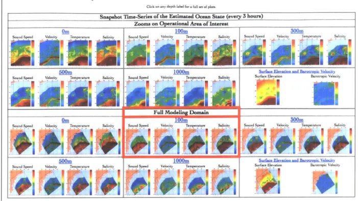
e Step 3: select the corresponding domain and depth. This page arranges data

according to the domain of interest (full domain or zoomed area) and depth

below the surface of the ocean. In this example, the user selects full-domain

and 100 m depth as shown in Figure 3-4.

Analysis and Forecasts for 26 Feb OOOOZ to 28 Feb OOOOZ 2017, Issued 26 Feb 2017

Click on any depth label for a full set of plou.

snaehot T.-serie. of the Estimated Ocean Stats_(eveg 3 hours)

Zooms on Operational Area of Interest

__

Sound Speed Velc y Temperature Salini y Sound Speed Velocit Temperature Saliniy Sound Speed Velocity Temperature Salinity

500M

1000M

Sound Speed Vi ociy Temperature Salinity Sound Speed Velocity Temperature Saie ty Surface Elevation Brr* Velocity

Figure 3-4: Domain and Depth [ll

SStep 4: select the desired data variable. This page lists the different modeled

Analysis and Forecats for 26 Feb OOOOZ to 28 Feb 0000Z 2017, Issued 26 Feb 2017

0100M

Sad Spmd

rip

Figure 3-5: Data Variable [1]

* Step 5: select the desired time. This page arranges the temperature maps

by their time stamp. The difference between each two consecutive thumbnails

correspond to a period of 3 hours. In this example, the user selects the fifth

thumbnail because the first one corresponds to 00:00 a.m. and they are

inter-ested in the profile at 9 a.m. The selected time thumbnail is shown in Figure

3-6.

ii

I

ii

I

Xa

Figure 3-6: Time Thumbnails [1]

9 Step

6:

visualize the data. This page shows a png (portable networks graphic)

or a graphics interchange format (gif) generated by MATLAB or NCAR. The

graphic plots a colormap of the temperature field in the full domain. It also

features a date and time stamp, longitude and latitude lines, extrema

informa-tion, and a well-defined color legend. The image of this example is shown in

Figure 3-7.

76W

70W

68W

-j

77

42N

Min= 7.6443E+00 Max- 2.3726E+01

1.38 Day Forecast : 9:00:00 26 Feb 2017

Figure 3-7: Desired Temperature Field 11]

As we have seen, the web experience is not very friendly as the user must return

to different webpages if they're interested in changing a parameter such as time,

depth, or the desired field. This necessitates a more intuitive approach that captures

variables in a multi-layered platform and allows the user to make quick conclusions.

This is why we designed user-controlled multi-layered multi-variable web maps.

7VW 68W 76W 74W 72V

23.0

22.1

21.3

20.4

19.6

18.7

17.9

17.0

16.2

15.3

14.5

13.6

12.8

11.9

11.1

10.2

9.4

8.5

7.6

Bibliography

[1] Multidisciplinary Simulation Estimation and MIT Assimilation Systems MSEAS. http://msea.s.mit.edu/.

[2] Deepak Narayanan Subramani. Probabilistic regional ocean predictions:

stochas-tic fields and optimal planning. 2018.

[3] P. F. J. Lermusiaux. Uncertainty estimation and prediction for interdisciplinary ocean dynamics. Journal of Computational Physics, 217(1):176-199, 2006. [41 Pierre F. J. Lermusiaux, P. Malanotte-Rizzoli, D. Stammer, J. Carton, J.

Cum-mings, and A. M. Moore. Progress and prospects of U.S. data assimilation in ocean research. Oceanography, 19(1):172-183, 2006.

[5] P. F. J Lermusiaux. Adaptive modeling, adaptive data assimilation and adaptive sampling. Physica D: Nonlinear Phenomena, 230(1):172-196, 2007.

[6] Geospatial big data: Challenges and opportunities. Big Data Research,

2(2):74-81, Feb 2015.

[7] http://ngwww.ucar.edu/whatisncarg.html.

[8] Advanced lagrangian predictions for hazards assessments (nsf-alpha): https://goo.gl/b2alky/. MSEAS-MIT.

[9] Precision ocean interrogation, navigation, and timing (point) posydon-mit-bbn: http://mseas.mit.edu/research/posydon-point/. MSEAS-MIT.

[10] Northern arabian sea circulation - autonomous research: Optimal planning sys-tems (nascar-ops): http://mseas.mit.edu/research/nascar-ops/. MSEAS-MIT.

[11] P. F. J. Lermusiaux, P. J. Haley, Jr., S. Jana, A. Gupta, C. S. Kulkarni, C. Mirabito, W. H. Ali, D. N. Subramani, A. Dutt, J. Lin, A. Shcherbina,

C. Lee, and A. Gangopadhyay. Optimal planning and sampling predictions for autonomous and lagrangian platforms and sensors in the northern Arabian Sea.

Oceanography, 30(2):172-185, June 2017. Special issue on Autonomous and

La-grangian Platforms and Sensors (ALPS).

[12] Mseas sea exercises. vorticity: https://goo.gl/2u8cuk, backward ftle: https://goo.gl/qhskbw, standard deviation of sound speed: https://goo.gl/u8ujof, temperature: https://goo.gl/tb6cqa.

Chapter 4

Map Design and Implementation

The need for interactive maps that characterize ocean fields and their uncertainties was established in the previous chapter. This chapter discusses the engineering pro-cess adopted while designing these maps and describes, in details, the steps of the process from software selection to styling methods.

The process of selecting the appropriate software program and libraries to design the maps consists of identifying the desired features and capabilities, evaluating a list of options, and selection. Here, we discuss each step.

4.1

The Wishlist

The wishlist is a list of features and capabilities the map and the corresponding software library are expected to possess. In our project, the desired features are:

a. Lightweight maps: The web maps are expected to provide a fast user expe-rience and handle many users at the same time without affecting their perfor-mance rate.

b. Browser compatibility: The web maps and the coding software are expected

to be compatible across different browsers. Main browsers to be covered are Chrome, Internet Explorer, Firefox, Opera and Safari.

c. Mobile device friendliness: Having a mobile-friendly web map is of critical importance as smartphone traffic is rising to exceed desktop traffic. The product is also expected to run on different operating systems for mobile devices. d. Multidimensional visualization capabilities: In order to match the nature

of the ocean fields and uncertainties and their change with space and time, the used software library should support multidimensional capabilities.

e. Open source and mature library: It is important to use a software library that is open-source and that has extensive API documentation. The ability to reach out to library developers and a plethora of supporting plugins are fringe benefits.

f. Modern visuals: As discussed in good data visualization requirements, it is important that the used library supports modern-looking graphics.

g. Minimized disruption to existing processes and workflow: Although this seems to be a local concern, it is crucial to select a design process that causes minimal disturbance to the current data cycle in the MSEAS group. The data fields to be visualized are big data sets that are generated in the back end in a certain fashion. Building upon this fashion and expanding into the web requires certain capabilities discussed in the next section.

4.2

The Options

Similar to any engineering process, after identifying the needs and constraints of the problem, developing possible solutions and iterating over their end use are necessary to build a prototype. As a team in MSEAS, we considered and discussed several options for the flow of the data cycle. These are summarized below.

4.2.1

Option 1

MSEAS traditional data generation practice + a JavaScript mapping library. This involves:

1. Performing numerical computation locally in the back end: Performance en-hancing techniques such as optimized scripts and parallel analysis frameworks are considered.

2. Generating georeferenced data files of a certain format compatible with the used library: these are files that list the scalar quantities of an ocean scalar field at points in space (intersection of a latitude and longitude lines) and time, or the scalar quantities of the two components of an ocean vector field (e.g. barotropic and baroclinic velocities of the velocity vector field).

3. Saving the data files in a web directory (such as the MSEAS run PE directories)

4. Visualizing the data on web/mobile devices by writing a Javascript code that utilize the Leaflet mapping library and the d3.js data handling library.

4.2.2

Option 2

"On-the-fly" cloud computation + a JavaScript mapping library. This involves: 1. Moving the raw data to a server (or to the cloud)

2. Performing numerical computations on the cloud in response to a certain re-quest fired in a web/mobile device using (1) "xarray", a Python package that uses powerful N-dimensional variants of the pandas data structures [1], and (2)

"Dask", a parallel computing library for analytics [2].

3. Saving the output in georeferenced data files