Quantifying biologically and physically induced flow and tracer dynamics in permeable sediments
21
0
0
Texte intégral
Figure
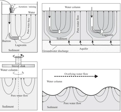
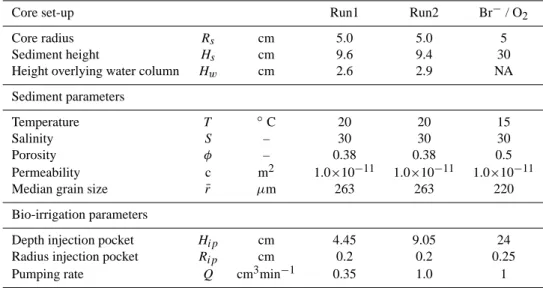
![Fig. 2. Model [1]: lugworm bio-irrigation in a laboratory core set-up. (a) scheme of the sediment domain geometry and the finite element mesh; (b) simulated flow line pattern; (c) simulated concentration pattern for the conservative tracer bromide after tw](https://thumb-eu.123doks.com/thumbv2/123doknet/14658393.553535/7.892.163.742.94.477/irrigation-laboratory-sediment-geometry-simulated-simulated-concentration-conservative.webp)
![Fig. 3. Model [2]: interaction between lugworm bio-irrigation and upwelling groundwater on a tidal flat](https://thumb-eu.123doks.com/thumbv2/123doknet/14658393.553535/8.892.203.698.95.401/fig-model-interaction-lugworm-irrigation-upwelling-groundwater-tidal.webp)
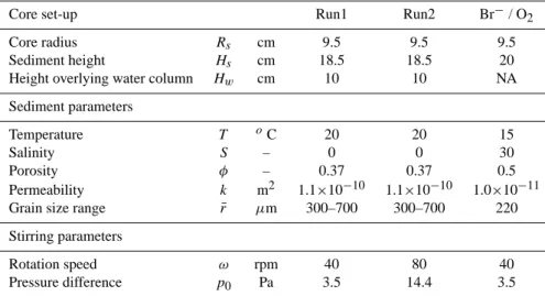
![Fig. 4. Model [3]: pore water flow induced in a stirred benthic chamber. (a) geometry of the sediment domain and the finite element discretization; (b) flow line pattern; (c) bromide concentration pattern after 12 h of incubation with the rotation speed of](https://thumb-eu.123doks.com/thumbv2/123doknet/14658393.553535/10.892.152.740.96.382/induced-stirred-geometry-sediment-discretization-concentration-incubation-rotation.webp)
+5
![Fig. 5. Model [4], laminar variant: Unidirectional flow over a ripple field with laminar flow conditions](https://thumb-eu.123doks.com/thumbv2/123doknet/14658393.553535/12.892.193.709.107.476/model-laminar-variant-unidirectional-ripple-field-laminar-conditions.webp)
![Fig. 7. Validation of the model [1] of the lugworm bio-irrigation.](https://thumb-eu.123doks.com/thumbv2/123doknet/14658393.553535/15.892.474.815.108.563/fig-validation-model-lugworm-bio-irrigation.webp)
Documents relatifs
