HAL Id: inserm-00188489
https://www.hal.inserm.fr/inserm-00188489
Submitted on 19 Nov 2007
HAL is a multi-disciplinary open access
archive for the deposit and dissemination of sci-entific research documents, whether they are pub-lished or not. The documents may come from teaching and research institutions in France or abroad, or from public or private research centers.
L’archive ouverte pluridisciplinaire HAL, est destinée au dépôt et à la diffusion de documents scientifiques de niveau recherche, publiés ou non, émanant des établissements d’enseignement et de recherche français ou étrangers, des laboratoires publics ou privés.
Model-based measurement of epileptic tissue excitability.
Paul Frogerais, Jean-Jacques Bellanger, Fabrice Wendling
To cite this version:
Paul Frogerais, Jean-Jacques Bellanger, Fabrice Wendling. Model-based measurement of epileptic tissue excitability.. Conference proceedings : .. Annual International Conference of the IEEE Engi-neering in Medicine and Biology Society. IEEE EngiEngi-neering in Medicine and Biology Society. An-nual Conference, Institute of Electrical and Electronics Engineers (IEEE), 2007, 1, pp.1578-1581. �10.1109/IEMBS.2007.4352606�. �inserm-00188489�
HAL author manuscript inserm-00188489, version 1
HAL author manuscript
Abstract— In the context of pre-surgical evaluation of
epileptic patients, depth-EEG signals constitute a valuable source of information to characterize the spatiotemporal organization of paroxysmal interictal and ictal activities, prior to surgery. However, interpretation of these very complex data remains a formidable task. Indeed, interpretation is currently mostly qualitative and efforts are still to be produced in order to quantitatively assess pathophysiological information conveyed by signals. The proposed EEG model-based approach is a contribution to this effort. It introduces both a physiological parameter set which represents excitation and inhibition levels in recorded neuronal tissue and a methodology to estimate this set of parameters. It includes Sequential Monte Carlo nonlinear filtering to estimate hidden state trajectory from EEG and Particle Swarm Optimization to maximize a likelihood function deduced from Monte Carlo computations. Simulation results illustrate what it can be expected from this methodology.
I. INTRODUCTION
D
uring, pre-surgical examination of epileptic patients, diagnostic is mainly based on merging information from anatomo-functional imaging, semiology and from electrophysiological signals recorded from scalp-electrodes (EEG signals) or depth-electrodes (SEEG signals). The latter capture important information about dynamical electrical activities arising from neuronal populations close to electrode contacts (2 mm long, 0.8 mm diameter for intracerebral electrodes). Interpretation of recorded signals is a crucial issue that is addressed, in this paper through modeling. The goal is to relate various temporal patterns observed in depth-EEG signals during interictal/ictal to modifications of model parameter values. These parameters can be interpreted in the model as pathological modifications of excitation and inhibition efficiencies. In order to establish such a relationship, parameters must be estimated from real observations. After description of the model (section II), we present a new identification methodology (section III) which is essentially based on likelihood computations through Monte Carlo (MC) sequential Bayesian filtering. In section IV simulation results are given and discussed before conclusion.II. MODEL DESCRIPTION
The model we introduce here belongs to the class of lumped-parameter models [1] introduced in the 70s to describe background activity or evoked potential responses.
Manuscript received April 16, 2007. P. Frogerais, J.J Bellanger and F. Wendling are with INSERM, U642, Rennes, F-35000, France; Université de Rennes 1, LTSI, Rennes, F-35000, France (corresponding author: +33 223 235 605; e-mail: [email protected]).
Here, it was adapted to hippocampus activity in epilepsy [6]. In the cortical tissue, distinct neuronal subpopulations types can be distinguished. The interactions between these subpopulations are either inhibitory or excitatory. The electrical activity they develop can be modeled as illustrated on fig. 1. Three subpopulations of neurons are considered: excitatory pyramidal neurons (Pe1 and Pe2) and two types of interneuron providing either slow dendritic inhibition (Psi) or fast somatic inhibition (Pfi). Coefficients Ci
correspond to (mean) numbers of synaptic contacts between subpopulations and are supposed known and time invariant. Each subpopulation module includes one (or more) linear filtering operator(s) whose output(s) is (are) applied to a nonlinear no memory operator S(.). This operator mimics threshold and saturation effects occurring at the soma. Input of filters and outputs of nonlinear operators represent the mean firing rate of action potentials. Outputs of filters represent excitatory or inhibitory (when weighted by -1) post synaptic membrane potentials resulting from time averaging in dendrites of impulse synaptic currents induced by afferent population(s). Biophysically, the EEG signal (field potential) recorded with an depth-EEG contact depends primarily on postsynaptic potential variations in Pe1 and Pe2 pyramidal cells. In such signal the influence of Psi and Pfi electrical activities can be neglected. Only three distinct transfer functions denoted he, hsi and hfi are introduced here. Their generic Laplace transfer function is
2 1 ( ) ( k ) h s s
τ
= + whereτ τ
= e,τ τ
= si orτ τ
= fi<τ
siare time constants whose respective values are fixed in accordance with those reported in literature [6]. Each transfer function introduces two scalar state variables. The influence of cortical neighborhood random activity on the four local subpopulations is resumed by a positive-mean time continuous Gaussian white noise W(t) applied on he input of Pe1 in addition to Pe2 output activity. The three
Model-based measurement of epileptic tissue excitability
P. Frogerais, J.J. Bellanger, and F. Wendling
S(.) C2 S(.) S(.) W + -A.he B.hsi G.hfi - + C6 B.hsi A.he A.he C5 A.he S(.) C7 C4 C3 Pe1 Pe2 Psi Pfi + + Physiological noise + + Model Output (EEG) V Instrumental noise Fs = 256Hz C1 S(.) C2 S(.) S(.) W + -+ -A.he B.hsi G.hfi - + C6 B.hsi A.he A.he C5 A.he S(.) C7 C4 C3 Pe1 Pe2 Psi Pfi + ++ + Physiological noise + ++ + Model Output (EEG) V Instrumental noise Fs = 256Hz C1
Fig. 1. The SEEG model.
positive parameters A, B and G are interpreted as positive synaptic excitation gain, synaptic slow inhibition gain and synaptic fast inhibition gain, respectively. These quantities are those we want to measure as they are supposed to vary during the transition to seizures. Therefore, the 3D parameter
3
( , , )A B G
θ= ∈ must be estimated from real signals in order to 'observe' these modifications. Finally instrumentation high pass filter and additive observation Gaussian noise are included in the model before sampling operator and the overall system can be written:
( ) ( ) t
dX = f X,θ dt G+ θ βd (1)
k k k
Y =HX +v (2)
where (1) is a vector (X∈ 14) stochastic differential equation (SDE) with a linear diffusion term G( )θ β and a d t
drift term f X( ,θ)dt. The Brownian motion increment t
d
β
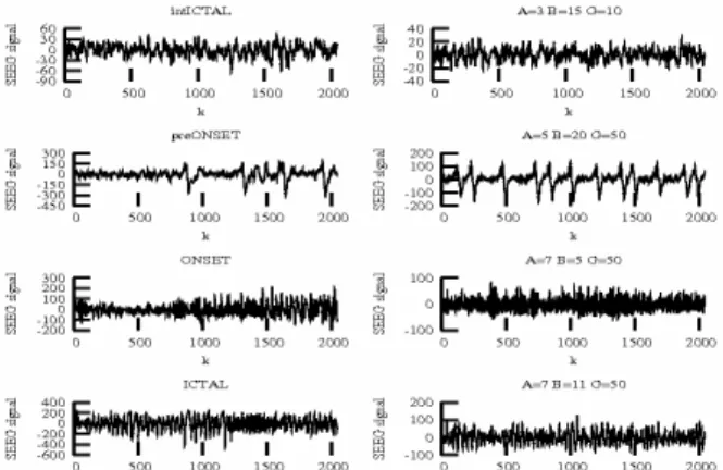
is the centered version of W t dt( ) . Vector X regroups state variables of subpopulation input filters plus two variables for the output high-pass filter. The function f accounts for i) nonlinearities (sigmoid S(.) functions), ii) transfer functions and iii) parameter θ. The output Yk is alinear form of sampled state vector Xk. In fig. 2 four real
depth EEG segments recorded before and during onset of a seizure (left) may be visually compared with model simulations (right) obtained with empirically adjusted values of (A,B,G).
III. IDENTIFICATION METHOD
A. Discrete scheme for the state equation.
To simulate time continuous SDE system (1) with discrete time observation (2), the SDE can be discretized by a second order Runge-Kutta method. In our particular model, we showed that this discrete approximation leads to:
2( 1 ) 2( ) (0 )
k frk Xk Grk Wk Wk N k
X = −, , ∆ +θ ∆,θ ∼ ,σ (3)
The two identification methods presented below and illustrated on fig. 3 use discretization (3) and equation (2).
B. First method: estimated moment method.
The first method involves only boxes b) and c) in figure
3). It consists in comparing estimated values
θ
ˆ with the observed sampled signal y1:N (modeled as an outcome of therandom vector Y1:N=[Y1,…,YN]) through a feature F(θ) define
as a functional of the probability law
1:N Y
Pθ . According to the moment parameter estimation method [8] an estimation
ˆ
θ
can then be defined as ˆ arg min ˆ( 1: ) ( ) NF y F
θ
θ = − θ
where F Yˆ ( 1:N) is an estimation of F(θ) computed on observation and . a quadratic norm. Here we retain
F=[F1,F2,F3] where the Fi,,i=1,2,3 are normalized expected
powers of four filtered versions of observation Y1:N
obtained by band-pass filtering through three frequency bands: delta (0-4Hz), theta and alpha (4-12Hz), beta and gamma (12-64Hz). As F(θ) can not be calculated analytically, we estimate it as function F yˆ (S S n1:S( , ))θ W of an outcome of model output (2) (nS time samples) simulated
with parameter value θ and input noise sequence W in (3). Because the function ˆ arg min ˆ( 1: ) ( )
N
F y F
θ
θ→ =θ − θ
may have several local minima a Particle Swarm Optimization Algorithm (PSOA) [7] is then utilized to compute
θ
ˆ(box c) fig.3).A PSOA is a global optimization procedure that propagates a set of K candidate
θ
valuesθ
kj,k=1..Kduring iterations j=1..J before stopping. At iteration j and for each particle k, its performance is valuated by computing Fig. 2. (left) segmented signals recording during an epileptic seizure.
(right) simulated signals by the model (Fig. 1) with different values of the parameters (A,B,G).
obser vation like lihoo d 1 2
c)
Par ticle Swar m Optimi zation Spec tral distance a) State and Like lihoo d computations b) Mode l sim ulation compu tations of PS D and of Spec tral distance
Fig. 3. The identification method.
Fig. 4. The function -h(θ,wk) calculated in the A-B plane (G=50) on a
realization of the second model (A=5, B=20,G=50).
1: 1: ˆ ˆ ( , ) ( ) ( ( , ) r k k j N S S n j h
θ
W = F y −F yθ
W which israndom since it depends on noise outcome W (Fig. 4 illustrates the effect of this randomness which entails difficulties to find an reliable optimum). For each j value the PSOA compute a small displacement for each particle as a function of its current position, of its position at preceding iteration and of best encountered positions in the past for itself and for a currently and randomly defined set of some other particles in the swarm (named advisors). The algorithm hence combines different randomly selected candidate values to produce new values in the same manner as evolutionary algorithms. It is stopped when h values became stable.
C. Second method: Maximum likelihood method.
This method involves mainly boxes a) and c) in fig.3). It necessitates an estimation L yˆ( 1:N, )
θ
of the likelihoodL(y1:N,θ) which cannot be computed analytically. This
approach was proposed in [1] for neural mass models simpler than our model (only three subpopulations) and in a non-pathological context: it consists in implementing a nonlinear Bayesian filter for state point estimation (a form of improved extended Kalman filter [9]) and to compute likelihood as a function of innovations (prediction errors of the observation) for each
θ
value. Here we propose to utilize a particle filter [2] which provide information concerning state conditional probability distribution given observations. Hence we compute the likelihood by mean of a particle filter included in a) fig.3) and values ofθ
that lead to large likelihood values are, as for the first method, obtained with a PSOA algorithm (c) fig. 3)). In order to limit the particle filter computational time, the parameter space research is reduced by forbiddingθ
values (action of b) on c) fig.3)) which do not respect the constraint -h(θ,W)>α where α is set to an empirical value (α= - 0.2). This constraint is faster to calculate than the particle filter.Non-linear Bayesian filtering methods [9] are used to
estimate the hidden state trajectory X(t) of a non-linear Markov system observed through a noisy no memory function y t( )=g X t noise( ( ), )of this state. In case of discrete time state evolution, these methods consist in estimating the probability density
1:
|
k k
X Y
p of the state Xk at
discrete time tk given discrete observations Y1:k . Generally it
is a difficult problem, which necessitate approximate numerical resolutions, as doing by particular filters. Particular filtering [3] is an application of a MC method called sequential importance sampling with re-sampling (SISR) algorithm. This recent and popular method sample at each time k a set ˆx , i=1,…,Nki s, from an auxiliary density,
the instrumental density q, and compute associated weights
i k
w . These weights may be chosen such that the expectation 1: [ ( k) | k] E f X Y can be approximated by 1: 1 ˆ[ ( ) | ] Ns i ( )i k k i k k E f X Y ω f x =
=
∑
for arbitrary f(.) when Ns islarge [2]. Hence, when Ns is large the information provided
by the set ( ˆi k
x , i k
w ), i=1,…Ns, is equivalent to the
1:
|
k k
X Y
p knowledge. A natural and classical choice for the instrumental law is
1
|
k k
X X
q= p − which correspond to the so-called bootstrap filter [3]. But for reasonable (not too large) Ns value degeneracy phenomena appear: after several
steps, only a very little subset of particles give valuable information on
1:
|
k k
X Y
p . So, we used here a more sophisticated importance law called optimal instrumental density [2]. Particle filtering with optimal importance density was applied to discretized version (3) of system (1).
Furthermore it can be shown [4] that the likelihood can be approximated by: 1 1 1 1 ˆ( ) log s N N i N k k i L y: θ w = = , =
∑ ∑
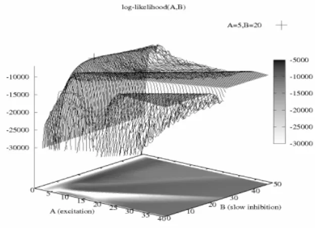
(4)To illustrate, fig. 5 shows estimated values of the log-likelihood as a function of (A,B) and with Ns=20 on a signal
simulated with θ =(5,20,50). G was set to its real value (G=50). We can notice several local maxima and the global maximum argument (the ML estimation) proximal to the real value (A=5,B=20).
IV. RESULTS ON SIMULATED DATA
We focused on four different models corresponding to four different activities shown in fig. 2 (right). For each model, ten realizations were simulated. Then the second parameter estimation method, presented in the previous section, was applied on these 40=10x4 signals, with Ns=20.
A 40 particles swarm with 3 advisors for each particle was used in the PSOA. Estimated parameter values are plotted in the parameter space, fig. 6. Different symbols are used to mark different models. Each set of links represents ten estimations obtained with ten output outcomes of a given model. We can note that, despite the estimation dispersion, Fig. 5. The log-likelihood calculated on a realization of the first model
A=5, B=20, G=50.
four sets can be easily distinguished. This shows the
relevance of the estimation procedure.
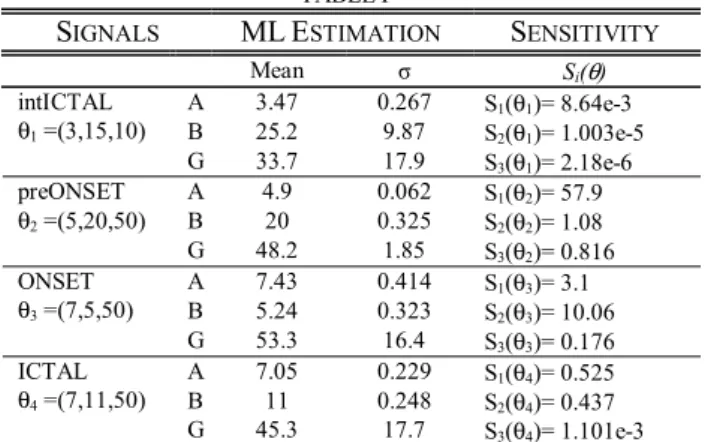
The experimental means and standard deviations of the four sets of parameter estimations are reported in table I. Except for the second model, the estimation of parameter G presents high variations. In the first model, B and G estimates have also a high variance.
In order to compare the two identification methods described in section III, parameters were estimated ten times for each model and for each of the two methods. For each model, this process was performed on the same simulated observation. The obtained experimental means and standard deviations are reported in table II. Globally the first
estimator shows more dispersion than the second one. This dispersion is due to the dependency on W of the feature vector estimate. It could be reduced by taking nS larger than
observation duration but it can be shown that this would also introduce bias.
For the second method, the MC sampling is the essential cause of dispersion. It can be reduced by increasing Ns and,
therefore, proportionally increasing the computational time. In order to numerically evaluate how a small variation ∆θ on parameters has an effect on the EEG output, we simulated, with two models: M1=M(θ) and M2=M(θ +∆θ) and for a
same realization W of input noise, two signals ys1:ns(θW)
and ys1:ns(θ+∆θ,W). An measure of the sensitivity is obtained
by calculating the mean square error between these signals:
2
1: 1:
( ) ( , ) ( , )
i s ns r s ns i r
S θ = y θ n −y θ+ ∆θ n (5)
for i=1,2,3 with ∆θ1=(0.2,0,0), ∆θ2=(0,0.2,0),
∆θ3=(0,0,0.2). An evaluation of this quantity for a
realization of each simulated model (fig. 2) is reported in Table I. Note that identifiability of the model increases when this parameter increases.
V. CONCLUSION
Results obtained on simulated signals show that estimation of synaptic gains is not easily achieved in some regions of the parameter space. Nevertheless, the ML method with MC approximation and particle swarm optimization we presented here makes this estimation feasible. The main difficulty before being able to apply it on larger databases is to address the problem of required computer time, more especially in case where model outputs are less sensitive to parameter vector values.
REFERENCES
[1] P.A. Valdes, J.C. Jimenez, J. Riera, R. Biscay, T. Ozaki “Nonlinear EEG analysis based on a neural mass model” Biol. Cybern. 81, 415-424 (1999)
[2] Olivier Cappé, Eric Moulines, and Tobias Ryden. Inference in Hidden Markov Models (Springer Series in Statistics). Springer-Verlag New York, Inc., Secaucus, NJ, USA, spinger edition, 2005.
[3] N.J. Gordon, D.J. Salmond, and A.F.M. Smith. Novel approach to nonlinear/non-Gaussian Bayesian state estimation. IEE Proceedings, 1993.
[4] M. Hürzeler and H. R. Künsch. Approximating and maximizing the likelihood for a general state-space model. 2001.
[5] Joshua Wilkie. Numerical methods for stochastic differential equations. Physical Review E (Statistical, Nonlinear, and Soft Matter [6] F. Wendling, A. Hernadez, J.J. Bellanger, P. Chauvel, F. Bartolomei
“Interictal to ictal transition in human temporal lobe epilepsy: Insights from a computational model of intracerebral EEG” JCN, 2005. [7] M. Clerc. Particle swarm optimization. ISTE, 2006.
[8] B Porat., Digital processing of random signals, Prentice-Hall, 1994. [9] A. H. Jazwinski, Stochastic processes and filtering theory, Academic
Press, 1970. TABLEI
SIGNALS ML ESTIMATION SENSITIVITY Mean σ Si(θ) A 3.47 0.267 S1(θ1)= 8.64e-3 B 25.2 9.87 S2(θ1)= 1.003e-5 intICTAL θ1 =(3,15,10) G 33.7 17.9 S3(θ1)= 2.18e-6 A 4.9 0.062 S1(θ2)= 57.9 B 20 0.325 S2(θ2)= 1.08 preONSET θ2 =(5,20,50) G 48.2 1.85 S3(θ2)= 0.816 A 7.43 0.414 S1(θ3)= 3.1 B 5.24 0.323 S2(θ3)= 10.06 ONSET θ3 =(7,5,50) G 53.3 16.4 S3(θ3)= 0.176 A 7.05 0.229 S1(θ4)= 0.525 B 11 0.248 S2(θ4)= 0.437 ICTAL θ4 =(7,11,50) G 45.3 17.7 S3(θ4)= 1.101e-3
Parameter estimation on ten simulated signals for different activities
(models) (intICTAL, preONSET, ONSET, ICTAL). Fig. 6. Results of parameter estimation with simulated data. Ten signals were simulated by the model for 4 different values of theta corresponding to the different cases on the Fig. 1.
TABLEII
SIGNALS ML METHOD MOMENTMETHOD
Mean σ Mean σ A 3.42 0.338 16.26 9.24 B 29.96 13.2 15.9 7.71 intICTAL (3,15,10) G 53.6 20.5 38 31.6 A 4.92 0.0362 5.72 0.375 B 20.8 0.143 24.2 2.36 preONSET (5,20,50) G 50.5 0.995 64.8 12.6 A 7.38 0.713 23.9 6.71 B 5.06 0.663 6.72 2.03 ONSET (7,5,50) G 50.8 27 48.8 12.3 A 7.2 0.436 11,1 24,3 B 11.4 0.430 24,3 29,9 ICTAL (7,11,50) G 34.4 18.2 29.9 8.2 Comparison of two parameter estimation methods computed 10 times on the same simulated signal. The real parameter values are in brackets.