The design and implementation of a synchronous manufacturing system in a job-shop environment

THE DESIGN AND IMPLEMENTATION OF A SYNCHRONOUS MANUFACTURING SYSTEM

IN A JOB-SHOP ENVIRONMENT by

JEFFREY L. ALCALDE

B.S., Civil Engineering, University of California, Berkeley, 1992

Submitted to the Department of Civil and Environmental Engineering

and the Sloan School of Management

in partial fulfillment of the requirements for the degrees of

and

MASTER OF SCIENCE IN MANAGEMENT

IN CONJUNCTION WITH THE LEADERS FOR MANUFACTURING PROGRAM AT THE MASSACHUSETTS INSTITUTE OF TECHNOLOGY

June 1997

@ 1997

Massachusetts Institute of Technology. All rights reserved.

Signature of Author _ _ __,_

u o MIT Sloan School of Management Department of Civil and Environmental Engineering

June 1997

Certified by

Stephen Graves, Professor

Co-Director, Leaders for Manufacturing Program Thesis Advisor Certified by

Joel Clark, Professor Department of Material Science Thesis Advisor Certified by

David H. Marks, Professor Department of Civil and Environmental Engineering Thesis Reader Accepted by

"a ' UJJgep M. Sussman

Chairman, DepartmentaL rnmittee dGrfduate Studies

Accepted b. o

0 _{0c , Jeffrey Barks}

Associate Dean, Sloan Master's and Bachelor's Programs

JUL 0 11997

THE DESIGN AND IMPLEMENTATION

OF A SYNCHRONOUS MANUFACTURING SYSTEM

IN A JOB-SHOP ENVIRONMENT

by

JEFFREY L. ALCALDE

Submitted to the Department of Civil & Environmental Engineering and the Sloan School of Management June 1997

in partial fulfillment of the requirements for the degrees of

MASTER OF SCIENCE IN CIVIL AND ENVIRONMENTAL ENGINEERING

and

MASTER OF SCIENCE IN MANAGEMENT at the

MASSACHUSETTS INSTITUTE OF TECHNOLOGY

ABSTRACT

This thesis presents how a company can design a synchronous manufacturing system in an environment as complex as a large job shop. Because the job shop has many unique features such as shared processing resources over many product lines and the fact that many of the products are made to order, it is not feasible to use existing literature with regards to synchronous manufacturing systems on single product lines. This thesis uses the theory of constraints as proposed by Eliyahu Goldratt as a baseline and then modifies its use to meet the needs of the large job shop.

When analyzing the large job shop using the theory of constraints, one finds that constraints are defined as much by manufacturing policy as by process capacities. This combination of policy and process constraints creates the need to define several types of constraints. These constraints are single product constraints, multiple product constraints, and plant capacity constraints. An increase in the capacity in each of the types of constraints results in different benefits to the plant.

In addition to using the theory of constraints to analyze throughput, the thesis analyzes inventory management using Goldratt's drum-buffer-rope system. This system allows for the development of tools which can be used to continuously improve the synchronous manufacturing system. In order to measure the benefits of a synchronous manufacturing system, the thesis calculates several costs, such as inventory holding costs, inventory obsolescence costs, strategic costs, quality costs, and environmental costs. All costs are calculated in dollars with the exception of environmental costs which include mass of air emissions as well as utility dollar costs.

Finally, the thesis asserts that, in addition to designing a synchronous manufacturing system for the large job-shop, there are many difficulties in implementation. The thesis claims that changing from a batch and queue manufacturing system to one of synchronous manufacturing is a change of corporate culture and manufacturing strategy and therefore must be supported by an entire change in thinking which values systematic thinking to increase manufacturing flexibility in addition to traditional throughput oriented values.

THESIS ADVISORS

Dr. Stephen Graves, Professor of Management Dr. Joel Clark, Professor of Material Science

A

First, I wish to thank my family for supporting me in my efforts over my entire lifetime. Both of my sisters, Keri and Lisa, have listened to me when I needed support and inspired me. My parents, Herman and Sherry have been so loving and encouraging that there is no way in which I can return their favor over my lifetime. I only hope that I can provide as much support, guidance, and inspiration to the people I come in contact throughout my life. I also wish to thank my Grandfather, Herman Alcalde Sr. for the laughs and the love he gave his grandson throughout his lifetime.

I would also like to thank Steve Graves and Joel Clark, my advisors at MIT, for their guidance and support during this research effort. Their support was critical to its success. Without the support of everyone at Alcoa, I would have never been able to achieve as much as I did over such a short period of time. The atmosphere they provided was one of openness, change, and enthusiasm both in helping me understand the workings of their plant and in listening to the ideas I presented. I specifically wish to thank TPK, RGM, JVV, BSB, KES, and JPD. Unfortunately, it is not possible to mention all of the people who shared with me their knowledge and support, but they are definitely remembered and thanked.

I am thankful to have been a part of the LFM Class of 1997. I will remember you all with such fondness. You are all amazing people who have graciously shared your knowledge, experiences, and smiles. I hope that I have given as much to you all as I have received from you. I especially want to thank Ms. Joetta George for brightening my life for the past two years.

I gratefully acknowledge the support and resources provided to me through the Leaders for Manufacturing Program, a partnership between MIT and major U.S. manufacturing companies.

TABLE OF CONTENTS Abstract 3 Acknowledgments 5 Table of Contents 7 CHAPTER 1 -- INTRODUCTION 9 1.1 Plant Background 9

1.2 The Need for Change 10

1.3 Management's Support of Change 11

1.4 Thesis Organization 12

CHAPTER 2 -- SYNCHRONOUS MANUFACTURING THEORY 13

2.1 Theory of Constraints 13

2.2 Inventory Management 14

2.2.1 Single Piece Flow 15

2.2.2 Drum-Buffer-Rope 17

2.3 Summary 19

CHAPTER 3 -- APPLICATION OF THE THEORY OF CONSTRAINTS 21

3.1 Identifying Flowpaths 22

3.1.1 Material Defined by Products and Markets 22

3.1.2 Material Defined by Manufacturing Process 23

3.2 Types of Constraints 23

3.2.1 Single Product Constraints 24

3.2.2 Multiple Product Constraints 24

3.2.3 Plant Capacity Constraints 25

3.2.4 Non-Constraints 25

3.3 Analysis of Tim's Metal Finishing Company 26

3.3.1 Determining Flowpaths 26

3.3.2 Analyzing Each Process 33

3.3.2.1 Initial Cleaning 34

3.3.2.2 Metal Softening 34

3.3.2.3 Machining 34

3.3.2.4 Deburring 35

3.3.2.6 Surface Preparation 35

3.3.2.7 Inspect/Test 36

3.3.2.8 Painting 36

3.4 Summary 36

CHAPTER 4 -- INVENTORY ANALYSIS 39

4.1 Purpose of Inventory 39

4.2 Effects On Inventory 40

4.2.1 Batch Processes 42

4.2.1.1 Costs of Batch Processes 43

4.2.2 Process Variability 44

4.2.2.1 Costs of Variability 45

4.2.2.2 Costs of Variability Example 45

4.2.2.3 Environmental Costs 47

4.3 Summary 52

CHAPTER 5 -- ON TIME DELIVERY 53

5.1 Special Issues Within a Job-Shop Environment 53

5.2 Scheduling and Order Processing 55

5.2.1 Production Capacity Vs. Product Variety 56

5.2.2 Measurement Systems 56

5.2.3 Machine Capabilities 58

5.3 Summary 59

CHAPTER 6 -- FLEXIBLE SYSTEM THINKING 61

6.1 Allocation of Capital 62

6.2 Measurement and Reward Systems 62

6.3 Expedited Batch Runs 62

6.4 Training 63

6.5 Scheduling Systems 64

6.6 Summary 67

CHAPTER 7 -- CONCLUSIONS 69

Chapter 1 -- Introduction

The theory of constraints [Goldratt and Fox, 1984] applies very cleanly when a manufacturing facility is structured by product or flow lines. In this case, a group of machines work together to produce a particular product or product family and no other. The constraint can be identified by its production capacity relative to the other machines in the product line. One of the main challenges of applying the theory of constraints in a job shop environment is that machines are constantly being shared between product lines or families. This is not a complication when the machine is a non-constraint. However, when the machine is a constraint, and it is shared between products, management policy regarding which products are more valuable becomes critical. This paper identifies

several unique aspects to the job shop environment and proposes ways to modify existing theories to meet those unique needs.

1.1

PLANT

BACKGROUND

The plant in this study is an Aluminum Company of America (ALCOA)

aluminum processing plant. The plant has been in existence for more than 50 years and has grown steadily during that time. The plant currently employs approximately 2,000 hourly workers.

As part of its growing process, the plant has had to endure many business cycles. In order to do so, management has made it a point to retain the capabilities for processing aluminum to suit many uses. In doing so, the plant is able to shift its production between markets as market demand changes, thus reducing the variability associated with a single market. Because of the large capital expenditures associated with increasing metal processing capacity, the plant has added one machine at a time as the need arose. This piecemeal growth, accompanied with the desire to manufacture a wide array of products, led the plant to grow as a job-shop, not as an increasing number of manufacturing lines.

Even as the 90's passed and a growing number of companies began to focus on particular markets well suited for their core competencies, management persists with its strategy of manufacturing a wide array of products. There is a strong belief within upper management that a diverse product mix offering will support the plant through future business cycles.

Along with realizing the advantages of providing a wide product range, management faces many of the challenges associated with operating a large job-shop. One challenge is that equipment is extremely costly, leading it to be designed and

operated to produce large batches, taking advantage of economies of scale. Additionally, because the plant is a large job-shop, the measurement systems that have been in place measure production at each individual machine. The more metal processed by a particular machine, the better the performance evaluation. This combination of large batch runs and local measurement systems lead to very large inventory and long lead times.

1.2

By choosing to provide such a wide variety of products, plant management has created a way to deal with business cycles. However, at the same time, management has created the risk of providing so many products that it is difficult to keep up with

increased competition for each product line. This large job-shop faces some business threat from other large plants producing a full array of products; however, those plants will face the same risks as the plant in this study. Similar to the large steel plants of the 70's, this plant faces a larger threat of becoming uncompetitive one product line at a time as numerous smaller competitors focus on producing and delivering a single product. Even though these smaller plants face the risk of supplying a narrower market, they are able to focus their efforts on creating value for a specific type of customer. At the time of this study, the plant was performing quite well, and not losing market share to smaller

producers; however, it is believed that small producers still present the largest long-term business threat to the large job-shop.

At the same time that competitors are focusing on taking business from the large job-shop, one product at a time, there is another factor pushing the need for change. Because customers are operating with less inventory themselves, they have been

requiring a broader variety of metal and have been ordering smaller batch sizes of metal delivered more frequently. These demands are very difficult for a plant to meet when its machines have been constructed to process large batch runs of a single product.

In order to face increased competition and to create the value its customers demand, the large job-shop must either focus on a smaller number of products or operate differently. Reducing the number of products produced eliminates the advantage of operating a job-shop and runs the risk of becoming a commodity, rather than a make to order, producer. Changing the method of operating, however, retains the job-shop advantage of producing a wide variety of products made to order and allows the plant to compete effectively with several different competitors at the same time. In smaller job shops, changing the method of operation may be relatively easily accomplished by moving or modifying old equipment. However, because, in the large job shop, it can be more expensive to move or modify current machines compared to purchasing new ones, it is forced to either work with the equipment in its current state or undertake costly capital improvements. This thesis explains how one can use the Theory of Constraints (TOC) and synchronous manufacturing theory [Umble and Srikanth, 1990], [Burgess and

Srikanth, 1989] to design and implement a synchronous manufacturing system within the constraints of the large job-shop.

1.3

At the time of this study, a new plant manager was in the process of transforming this job-shop to a series of flow shops. In the process, the traditional functional

organization of the past was flattened and transformed into a matrix type organization. This transition from job-shop to flow shop was underway at the start of this study and management was very supportive of the efforts, including my own, to analyze the plant as a system, make recommendations for improvement, and actually implement the

improvements. In short, the plant was under significant change, supportive of my efforts, and eager to hear of my findings.

1.4 THESIS ORGANIZATION

The lessons learned at the Aloca plant are applicable to the generic large job-shop. In order to provide clear illustrations of the learnings, the thesis creates a fictional

manufacturing facility referred to as Tim's Metal Finishing Company.

Chapter one provides the background of the plant on which this study is based as well as how changing competition and markets are forcing plants to change. Chapter two provides some background theory of Synchronous Manufacturing as developed by

Eliyahu Goldratt. Once the reader has an understanding of synchronous manufacturing theory, chapter three describes the specific application of synchronous manufacturing theory to the job-shop environment. In short it describes how to create and analyze virtual product lines within the job-shop. Chapter four provides an analysis of inventory costs and benefits. Chapter five provides the reader with an analysis of issues impacting on-time delivery. Chapter six addresses some of the cultural issues with implementing such a large scale change. Chapter seven provides a summary and conclusions of this paper.

Chapter 2 -- Synchronous Manufacturing Theory

This chapter provides the reader with some background in the field of the Theory of Constraints as advanced by Eliyahu Goldratt. [Goldratt and Fox, 1986] It is essential that the reader is somewhat familiar with these ideas as they are the foundation of the analysis applied in this paper.

2.1

The Theory of Constraints is based upon the belief that there is a single factor which restrains the advancement of an entire system. If we are able to identify that factor and improve it, the entire system will improve. Additionally, improvements made in factors which are not the restricting one will result in little or no improvement to the entire system.

One popular example of the theory of constraints is an analogy to a troop of marching soldiers. The goal of this troop is to march from one location to another as quickly as possible. However, the entire troop does not arrive at its destination unless every soldier does. Therefore, in order to improve the ability of the troop to march to its final destination, we need to increase the speed of the slowest soldier. If we increase his/her speed, we increase the ability of the entire troop to march more quickly.

Likewise, if we increase the speed of a soldier who is not the slowest, the speed of the entire troop will not increase.

We can expand the analogy of the troop of marching soldiers to explain some of the workings of a manufacturing facility. Much like the troop of soldiers who each must

cover a portion of ground before the troop covers that ground, a manufacturing facility must perform a series of processes before it can sell a finished product. Additionally, just as the first soldier must cover ground before any other soldier can, the first manufacturing process must be performed before any other can proceed. In other words, the

manufacturing process as well as the troop of soldiers has a designated ordering to it. So, as a troop of soldiers increases its speed by increasing the speed of its slowest soldier, a manufacturing facility increases its throughput by increasing the throughput of the process with the least capacity.

2.2

Historically, manufacturing companies have placed high emphasis on throughput issues for you cannot sell what you cannot make. However, until relatively recently, American manufacturing companies have not placed as much emphasis on inventory management. But, as competition has increased and power has shifted from sellers to buyers, the importance of inventory has risen for several reasons.

When there are more suppliers of a product, buyers can afford to be more selective as to the products they purchase. This has forced companies to offer a much wider selection of product lines as the "one size fits all" products lose their advantages. Offering a wider variety of products means that companies must manufacture a wider variety of products. However, customers tend to buy a variety of products at the same time whereas manufacturing tends to produce a single product at a time. In order to deal with this issue, suppliers have chosen to hold a large amount of inventory. Inventory causes delays in the responsiveness of manufacturing as companies must "fill the distribution pipeline" every time they change a product line. This is critical for companies where time to market is important. These delays often result in excess of product that is not in demand and stockouts of high demand products, both of which result in less customer value and increased finished goods inventory at the plant. Short lead times allow a plant to counter this effect. Additionally, the amount of inventory is directly proportional to the amount of time it takes a company to deliver special ordered products (Little's Law). Shorter lead times can create value for customers by allowing quicker delivery as a variety of factors contributing to delays are reduced.

Another disadvantage of carrying inventory is it reduces product quality by causing feedback delays in the manufacturing and sales information, which is critical to operating a manufacturing plant. If there is a week of inventory between two processes, the downstream process will not learn of any defects until a week after they have been created. This makes it very difficult to find the cause of the defect. Additionally, there is a good chance that much, if not all, of the inventory between the two processes is

defective. A plant with less inventory is much more likely to find the cause of its quality problems and correct them when compared to a plant with high inventory and long feedback delays. More so, the plant with less inventory will have fewer defective parts when a quality problem should occur.

One final reason for carrying as little inventory as possible is that inventory is expensive to carry. By reducing inventory, companies are able to convert inventory to cash and increase their working capital. Most companies have determined a "cost of holding inventory" (expressed in percentages per year) which they feel is indicative of their cost of capital as well as some of the risks listed above. The purpose of this section is not to discuss the accuracy of the percentages, but to acknowledge that holding

inventory incurs costs.

2.2.1 Single Piece Flow

Recently, there has been much written concerning cellular manufacturing and single piece flow of material through a plant [Costanza, 1994], [Womack, 1996]. Whereas there have been several companies which have been successful at reducing product lead times and increasing product quality by converting to cellular manufacturing and single piece flow, there are several other companies which face difficult challenges in

implementing a system such as this.

A cellular manufacturing system assumes that a plant will have a group of

is relatively easy to accomplish if a facility produces a small product range or if it is possible to purchase several small machines with the same capabilities and equivalent price of large capacity equipment, for the job-shop environment there are several

difficulties. One such difficulty is that the very strategic strength of a job-shop is that it is able to produce a wide variety of products. Restricting the amount of products a job shop is willing to produce in order to achieve cellular manufacturing may undermine one of the plant's overall strengths. Another difficulty some job-shops lies in the fact that most of the current capital is very expensive and has been designed and built to process material

in very large batches. In order to implement cellular manufacturing, the plant would have to redesign and repurchase much of its capital base. For capital intensive industries, such

a large change may be too expensive. This is not to say that cellular design should not be considered for large job-shops. Large job-shops must consider smaller, more flexible machinery for any future capital expenditures, but to replace all current capital is prohibitive.

Another necessity of cellular manufacturing is that the machines are located near each other in order to form the cell. For some pieces of equipment, it may be relatively routine to move them about. However, for large pieces of equipment, it may cost several million dollars to move a single piece of equipment much less an entire plant. The cost of moving equipment can restrict a facility's ability to achieve cellular manufacturing.

In summary, cellular design has proven to be very effective in reducing lead times, improving product quality, and increasing flexibility and should be considered for any future capital expenditures. However, this conversion may take an extremely long time if most capital in place is durable. For the large job shop environment, a solution which is less capital intensive and is possible to implement in a shorter time horizon is needed.

2.2.2 Drum-Buffer-Rope

One inventory system solution which is applicable to the large job shop has been designed and called "Drum-Buffer Rope"(DBR) by Eliyahu Goldratt. In order to

understand the ideas behind it, we once again return to the analogy of a troop of marching soldiers.

For the troop of marching soldiers, the amount of inventory in a plant is

represented by the spreading of the soldiers. The larger the distance from the first soldier to the last, the larger the "inventory" of the troop. This raises the question, "How do we allow the soldiers to march as quickly as possible in as tight a formation as possible?". One solution to this problem has been to tie each of the soldiers together. By doing this we predetermine the largest distance the troop is allowed to spread. However, we have also created a tie between two soldiers neither of which is our slowest soldier.

Remembering that it is the slowest soldier which determines the maximum speed our troop marches at, these ropes may create an artificial constraint on the troop.

Transferring this analogy to a manufacturing plant, tying a rope between soldiers is analogous to setting a maximum inventory between each machine, with the length of each rope being the amount of possible inventory between any two processes. This system has been very successful in Japan and is called a Kanban system.

The DBR system is an extension of the Kanban system. Rather than tying soldiers together, another way to keep them from spreading is to give the slowest soldier a drum. As the slowest soldier moves, he beats the drum so that all other soldiers know the pace of the unit. This keeps the other soldiers from moving at their own pace and

spreading out the troop. Additionally, the troop can only move as quickly as the slowest soldier does. In order to prevent variations in the speed of the soldiers in front of the slowest soldier from slowing down the slowest soldier, we include a buffer space in front

of the slowest soldier. This way, if one of the faster soldiers should stumble and regain himself before the slowest soldier's progress is hindered, there will be no effect on the troop's speed. However, we do not want the soldiers to spread indefinitely, therefore we

must have some limit to the buffer. In order to control the spreading of the troop, we can attach a rope from the slowest soldier to the first soldier. We have now effectively limited the spreading of the troop. Additionally, we do not have to worry about the soldiers behind the slowest soldier because, although they will spread some due to variations in individual speed, they have the capability of catching the slowest soldier (and therefore the troop) if they fall behind, but they will never impede the speed of the slowest soldier. Note that if all soldiers were tied together, such as the Kanban system, two soldiers behind the slowest soldier have the ability of unnecessarily stop the troop if they should stumble.

Expanding this analogy to the manufacturing environment provides us with the basis for a powerful inventory management system. In section 2.1, I have discussed the Theory of Constraints. The constraining machine in the plant is analogous to the slowest soldier. Therefore, the pace of the constraint process should be the "drum" of the system dictating the pace of the entire plant. The "buffer" in the plant is the amount of inventory in the system which prevents the constraint from running out of work. This is the amount of inventory between the material release point (usually the first process in the plant) and the constraint. The "rope" dictates that this is a pull system. The amount of inventory between the material release point and the constraint has a maximum limit. As the constraint processes material, it will pull material from the material release point. The implications of this system are that there need only be tight control over material release and constraint operation. All other machines should process material until they run out of work.

One additional advantage the DBR method has over the Kanban method is the manner in which process variability is mitigated. DBR looks at all variability occurring between the material release point and the constraint as system variability whereas Kanban analyzes the variability between two processes regardless of whether one is the constraint or not. The effect of the DBR view is a smoothing of variability of process performance. Much like holding a diverse portfolio of stocks is less volatile than holding

an individual stock, the combined variability of all machines upstream of the constraint is less than the summation of the variability for each individual process. Therefore, in order to protect against variability, the DBR system holds enough inventory between the

material release point and the constraint to mitigate the system variability. In contrast, the Kanban system holds enough inventory to mitigate variability between each machine even when that variability has no effect on throughput.

2.3 SUMMARY

In this chapter, I have introduced the Theory of Constraints and the Drum-Buffer-Rope inventory management system as designed by Eliyahu Goldratt. The underlying concept of the theory of constraints is that there is a single factor which inhibits the performance of the entire system. If we can determine what this factor is, we can focus efforts to improve it and, thus, improve the performance of the entire system. If our efforts go towards improving non-constraining factors, we will have little or no impact on the performance of the entire system.

Whereas the Theory of Constraints is applicable to many manufacturing facilities, inventory control systems must be tailored to meet the specific needs of each

manufacturing plant and to each market being sold. One successful inventory

management system incorporates cellular processing and single piece flow. This system has been implemented in a number of facilities, but it presents some difficulties for plants which offer a wide variety of products and are capital intensive. Unfortunately, large job shops have both of these properties and therefore seek another system better suited to their needs. One such inventory management system is the Drum-Buffer-Rope system as it does not require the movement or purchase of new capital and is not limited by the size of the product line offered. The DBR system is based on the belief that the only reason to hold work in process (WIP) inventory is to keep the constraint from running out for work. For this reason, the two main issues are the system WIP before the constraint and the

throughput of the constraint. All other machines simply operate until they run out of work.

Chapter

3 -- Application of the Theory of Constraints

Understanding the Theory of Constraints allows one to conceptualize how a plant making a single product type would find its bottleneck (constraint) and design a DBR inventory system. Unfortunately, manufacturing plants are never this simple. Most make more than a single product and many have very difficult process flow diagrams. The term spaghetti diagram is sometimes used to describe these complicated process flow diagrams. The plant which this study is based on has very complicated process flows resulting in a large spaghetti diagram.

In order to provide an example of how to apply the theory of constraints in a job-shop environment, we will examine a fictitious company named Tim's Metal Finishing Company (Tim's). Tim's started out as a tool making facility consisting of many processes including metal softening, specialty cooling, machining, deburring, grinding, surface preparation, and painting. Additionally, some of Tim's newer products must be 100% inspected and tested whereas others have already had quality build in and therefore skip this step. As Tim's business increased, it became apparent that there was demand for specific processes Tim's performed aside from demand for tools, specifically metal softening and surface preparation. Tim's decided to perform some contracting for these services in addition to producing tools. As Tim's is currently operating as a job-shop, it is suffering from high inventory, long lead times, and poor delivery performance.

When analyzing Tim's as a group of machines which process parts independently, it is difficult to see how production at one resource effects the production of another. "Wandering bottlenecks" and "difficult product mixes" are used by Tim's workers to explain why production capacity seems to vary widely. However, by looking at Tim's as different "product lines" rather than a single group of machines, we are able to gain a much greater understanding of it as a manufacturing system.

This chapter provides an example of applying TOC to Tim's as well as the special modifications one can make to TOC in order to tailor it to this job-shop environment.

3.1

One of the first difficulties in applying TOC to a job-shop is that there are several different processes material undergoes depending on the final product. In order to handle this difficulty we must group our products together depending on what processes they undergo. In other words, we must separate our soldiers into different troops. Each combination of processes is called a flowpath. Flowpaths are "virtual processing lines" comprised of each machine used in the manufacturing process (in the order in which it is used) and treated as a single manufacturing line (although the machines may not be physically located near one another and only a portion of a machine's capacity may be needed for a particular processing line).

Tim's has historically identified flowpaths depending on the customer of the tool (for example general distribution, Sears, and contract work), not depending on what processes are performed. Although the customer is a decent proxy for the processes performed, it can sometimes disguise what the true constraint of a flowpath is.

3.1.1 Material Defined by Products and Markets

Tim's defines its products depending on the customer to which the product is going to be shipped. Those customers are: general distribution, Sears (Tim's has a large Sears contract), and contract work. However, these customers do not map perfectly into process flow paths. For example, some general distribution products are softened, cooled, ground, and painted, whereas other general distribution products are softened, cooled, and ground, but not painted. Additionally, some contract work falls under three different flow paths. This may not make much difference to the marketing department

when it forecasts demand for contract work, but it makes a huge difference in production

as grinding can process 250 parts a day, but painting can process only 50.

3.1.2 Material Defined by Manufacturing Process

In contrast to defining product families based on the customer, it is possible to define products by what processes are required to make them. I believe that this is a better way to analyze the system for the purpose of manufacturing planning of the products.

Referring back to the troop analogy, the first step is to identify which soldiers comprise which troops. It is impossible to determine what the constraint of the system is unless the system is defined accurately. By defining the flowpaths based on processes rather than customer, we can obtain accurate results for both the capabilities of the current system as well as performing "what if' scenarios for future planning. Defining flowpaths is done by determining all combinations of processes performed in the plant. For

example, a plant may have four processes called A, B, C, and D. Some products are processed by A and then either C or D. Other products are processed by B and then either C or D. This plant would have four flowpaths, AC, AD, BC, and BD.

Once flowpaths have been determined, one identifies the constraint for each flowpath based on processing capacity. Then, one combines flowpaths with the same constraint into a single flowpath. Finally, one checks to ensure that the demands of all constraints do not exceed the capacity of the processes which were non constraints on any single flowpath.

3.2 TYPES OF CONSTRAINTS

Another difficulty one encounters when applying TOC to Tim's is that not only are there many constraints due to the fact that Tim's produces many products, but there

are different types of constraints resulting because limited machine capacity is shared between several flowpaths. The idea of marginal machine capacity is important when analyzing shared resources. Over the course of this study, the different constraints displayed specific properties. I have identified the different constraints by their properties.

3.2.1 Single Product Constraints

There are constraints which touch only a single flowpath. These are identified as

single product constraints. A single product constraint determines a plant's capacity of a

single product type only. It is important to identify single product constraints because any increase of decrease in their capacity (marginal capacity) will change the plant's ability to manufacture products which fall on that particular flowpath. At Tim's, painting and inspect/test are examples of single product constraints. If Tim's were to increase painting capacity, we could make more paint constrained products, but not more grinding constrained products.

3.2.2 Multiple Product Constraints

There are constraints which touch multiple flowpaths. These are identified as

multiple product constraints. A multiple product constraint determines a plant's capacity

of more than one flow path. If a plant increases the capacity of a multiple product constraint and it is not fully utilizing a single product constraint on one of its flowpaths, the plant will have to choose on which flowpaths to increase throughput. However, if all single product constraints on the flowpaths are fully utilized, increases in multiple

product constraints will result in increased throughput only on the flowpath for which the multiple product constraint is the constraint. At Tim's, grinding is an example of a multiple product constraint. If Tim's increases the capacity of the grinders, the sum of paint constrained products and grinder constrained products Tim's can produce increases. If the plant was not fully utilizing its paint capacity, it can choose whether to produce

more paint constrained or grinder constrained product. However, if painters are fully utilized, increasing grinding capacity will result in increased throughput on the grinding constrained flowpath only. Once again, it is important to ask the question, "What result is the marginal increase/decrease in capacity going to allow the plant to achieve?".

3.2.3 Plant Capacity Constraints

If a constraint limits the amount of total product a plant can produce, it is aplant

capacity constraint. At the beginning of this study, I struggled with the question of why

increasing the capacity of a constraint might not lead to increased overall plant capacity. As the study progressed, it became apparent that some constraints restricted the plant's ability to offer a specific product mix; however, those constraints may not restrict the plant's total throughput.

In the discussion of single and multiple product constraints, the ability to increase overall plant throughput was not discussed. This is because whether a production center is a single product constraint or a multiple product constraint is independent of whether it is a plant capacity constraint. A constraint can be both a single product or multiple

product and a plant constraint.

The reason these two ideas are independent is, once again, due to the fact that a job-shop shares production center resources among its flowpaths. Increasing the

throughput capacity of one flowpath may require taking constraint capacity from another flowpath. This results in the ability to make a wider product mix, but no net increase in plant capacity.

3.2.4 Non-Constraints

In some senses, non-constraints is a misnomer. It is true that there are many production centers which have more processing capacity than is needed at this time.

However if there were demand for a product which used only non-constraint production centers, the plant should seriously consider making that product for the costs of doing so are low (materials and labor) and there will be no need to reduce production of any other product. Assuming management would produce this product if there were sufficient demand for it, I believe that demand constrained is a more accurate term; demand for the product (the market), not any of the processes, restricts its production. A machine is demand constrained if it is capable of producing more product than the market will bear. These machines are frequently called non-constraints.

One of the important adaptations of TOC to a job shop environment is the idea that management policy as well as machine capacity determines constraints. In addition to demand constrained processes, there may be processes which management has intentionally chosen to starve. For example, it may be more profitable to produce on a flowpath which has a multiple product constraint than to produce on a flowpath with a single product constraint. It is possible to allocate so much of the multiple product constraint's capacity to its flowpath so as to starve the constraint on another flowpath. A machine is starved if it is the constraint for a particular product type but is not fully utilized so that more of another product type can be produced.

3.3 ANALYSIS OF TIM'S METAL FINISHING COMPANY

Now that the general principals which were discovered as part of this project have been discussed, this section provides a specific example of their application in Tim's Metal Finishing Company.

3.3.1 Determining Flowpaths

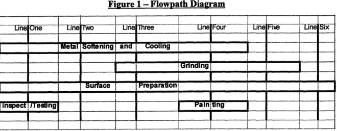
In order to determine the various product lines present at Tim's, the diagram shown in Figure 1 was constructed. The lines in the diagram are flow paths and show how material flows through the plant. If a line crosses a box labeled with a process name,

then the material in that product line is processed by that process. There should be a line for each combination of processes which make a final product. For example, there is one group of material which is processed through the metal softening, cooling, surface

preparation, and then inspect/test (labeled Line One). There is another group of material which is processed through metal softening, cooling, grinding, and then surface

preparation (labeled Line Three). Each of these lines represents the flow of a group of material.

Figure 1 - Flowpath Diagram

115- T 'Mf In m .

... So. ening a O. Cooling i

urface Preparation

InspectTesting Painting

The next step is to look at each line and determine which process on the flowpath has the least capacity. This process will be the constraint for that particular group of metal. For Tim's, the following capacities were used:

Metal Softening & Cooling -- 350 parts./day

Grinding -- 200 parts./day

Surface Preparation -- 650 parts/day

Inspect/Test -- 50 parts/day

Painting -- 50 parts./day

This results in the following combination of lines and constraints.

Line # Product Name Constraining Process Production Name

1 Contract Work Inspect/Test Inspect/Test Constrained

2 Contract Work Metal Softening Softening Constrained

3 General Distribution Grinding Grinder Constrained

4 Sears Painting Paint Constrained

5 Sears Grinding Grinder Constrained

(For clarity, I have labeled each line with its most appropriate "product name". However, as I have discussed in section 3.1.2, the most useful production name for each group is given by its constraining process, not by its end use.)

Finally, we can group all lines with the same constraint together to form flow

paths. At Tim's, we can group lines 3 and 5. This results in five different flow paths at

Tim's. Tim's employees comfortable working with product names might not want general distribution and Sears grouped together because one goes through metal softening and cooling and goes through a grinding process whereas the other is not softened and goes through a grinding process. However, both products demand resources from the grinders. It is important when booking the business to realize that different products consume different amounts of time on a constraint process so that a flow path does not become overbooked. However, once the business is booked, the capacity of the constraint is determined. The objective of the constraint is still to process as much product as possible and in the correct order regardless of whether the product is for Sears or for general distribution.

In order to implement a synchronous manufacturing system, it is important that the resources needed to produce the product are considered more so than the market in which the product will be sold. At Tim's, each product can be mapped into a particular flow path depending on which constrained process it flows through. At Tim's, all products fall into one of five categories listed below in order of descending processing capacity.

Surface Preparation constrained -- Products which do not pass through metal softening,

cooling, grinding, inspect/test, or paint.

Metal Softening Constrained -- Products which pass through metal softening and cooling,

Grinder Constrained -- Products which pass through grinding, but do not pass through painting.

Inspect/Test Constrained -- Products which pass through inspect/test.

Paint Constrained -- Products which pass through painting.

By looking at a product with regards to which flow path it maps into rather than by which market it serves, it is possible to determine how each process impacts the entire

plant production system. And, even more powerful, Tim's can now schedule production so that it benefits the entire plant operations rather than the operation of the single process in isolation.

One possible way to display the relevant data is shown in Figure 2. In Figure 2, we have created a grid layout in which graphs of cumulative monthly production at each process can be placed. All material flowing through the plant will be displayed on one of the horizontal flowpaths. By creating a matrix of data, with the flowpaths displayed horizontally and the production centers displayed vertically, it is easy to see how each of the processes is performing relative to the drum on each flowpath. Gray areas of the chart have no graphs as the flowpaths, by definition, do not have those processes on them. This information can help in determining which flowpath a process should be producing for in order to level production and ensure that a constraint does not become starved.

Figure 2

. I

I

o ... .... .... I.

i- Initial Cleaning Metal Softening: Grinding Surface Prep lnspect/Testi Paint

a.

Surface Prep

(Rope)

Grinding Material Release Constraint

Gri(Rope) nding

_(Rope)

_(Drum)

Material Release Inspect/Test

S (Rope)

Pt Material Release

Pa(nting

(Rope)

In addition to assisting process scheduling, the grid layout of cumulative monthly production graphs will display whether the material release point is changing the amount of WIP inventory in the system by releasing either more or less material than the

constraint on the flowpath has consumed. At Tim's, the material release point is initial cleaning.

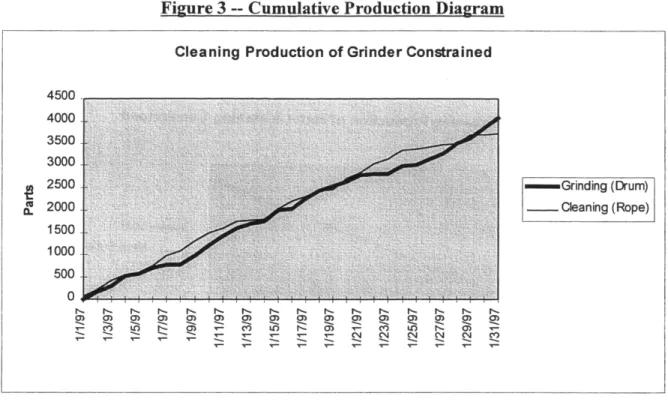
Figure 3 shows cumulative January initial cleaning for the grinder constrained flowpath. Analysis of this graph reveals that the initial cleaning process has released less material than the constraint has processed for the month of January. This would result in decreased inventory in the grinder constrained flowpath relative to the end of December inventory levels. Additionally, we can see that the material release rate as well as the grinder (constraint) production rate vary on this flowpath.

Figure 3 -- Cumulative Production Diagram

Cleaning Production of Grinder Constrained

4500 _ 4000 3500 3000 ~_ns 2500 2000 a. 1500 1000 500 0 ... ... ... ... ... ... ... ... ,... ,... ,... ,... ,... ... ... ,... Q? ~ ~ ~ ~ Q? Q? Q? Q? _§5 Q? _~ Q? m Q? Q? ... ... (") It) ,... ... It) r::: m

§

-

-

-

-

-

-

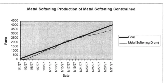
If we choose to analyze the production for a particular process, we can see how much capacity the process has allocated to each flowpath. Figures 4 through 7 display the metal softening cumulative January production on each of the four flowpaths which it produces. Figure 4 shows that metal softening produced less metal than was the goal for the metal softening constrained flowpath. Figure 5 shows that metal softening processed more metal than the grinder for the grinder constrained flowpath. This will increase the amount of inventory between the two processes, but will not alter the total inventory in the system as only the material release process effects system WIP. Figure 6 shows that metal softening produced roughly 500 pieces more than the inspect/test did on the inspect/test constrained flowpath. Figure 7 shows that metal softening produced approximately 400 pieces more than painting for the paint constrained flowpath.

If metal softening had used more capacity for the grinder and metal softening constrained flowpaths (assuming the demand existed for metal softening constrained pieces) and less on the inspect/test and paint constrained flowpaths, it would have assisted in leveling production at Tim's. And, the more level production is, the less

inventory the plant needs. Analyzing production by flowpath allows the plant to assist in leveling production over each flowpath.

Figure 4 -- Cumulative Production Diagram

Metal Softening Production of Metal Softening Constrained

4500 4000 3500 3000 ~ 2500 ~ 2000 1500 1000 500 o - G o a l

_ _ N'etal Softening Drum)

Date

Figure 5 -- Cumulative Production Diagram

Metal Softening Production of Grinding Constrained

4500 4000 3500 3000 ~_ns 2500 -2000 D. 1500 1000 500 0

""

"" "" "" ""

"" ""

""

-

-

-

-

-

Figure 6 -- Cumulative Production Diagram

Metal Softening Production of Inspect/Test Constrained

1800 1600 1400 1200 ~_nl 1000₈₀₀ a. 600 400 200 0 ... ... ... ... ... ... ... ... ... ... ... ... ~ _{~ ~} m ~ ~ _{~ ~} m ~ ~ ~ ....-

t:

-

....

-

Figure 7 -- Cumulative Production Diagram

Metal Softening Production of Paint Constrained

1800 1600 1400 1200 ~_nl 1000₈₀₀ a. 600 400 200 0 ... ... ... ... ... ... ... ... ... ... ... ... ~ m _~ ~ ~ ~ _~ m en _{~ ~} ~ ....- _~ LO ....- in r:: m

....--

-

-

- -

-

-

3.3.2 Analyzing Each Process

Determining the flowpaths of a production system provides the framework with which to analyze the system. This section provides an interpretation of the flowpath and constraint identification process as it applies at Tim's. Itis organized by process so that the impact each process has on Tim's can be examined.

3.3.2.1 Initial Cleaning

The capacity of cleaning is greater than the demands on them from each of the constrained processes; therefore, initial cleaning is a non constraint. Increased cleaning capacity will not increase plant capacity.

3.3.2.2 Metal Softening

Because metal softening produces on four flowpaths (paint, inspect/test, grind, and metal softening constrained) they are multiple product constraints. Much like the grinders, an increase in metal softening capacity will allow the plant to increase its total combined throughput of paint, inspect/test, grinder, and metal softening constrained products. However, the increase will not allow a flowpath's throughput to be greater than the throughput of its constraining process. For example, no matter how much metal softening capacity increases, the amount of paint constrained product produced cannot be greater than the capacity of the paint process. Again, much like the grinders, an increase in throughput on flowpaths which the metal softening process touches will result in increased demand for surface prep resources on those same flowpaths. This increased demand will reduce the amount of surface prep resources dedicated to the surface prep constrained flowpath resulting in no net throughput increase. Metal softening is not a plant throughput constraint.

3.3.2.3 Machining

The capacity of machining is greater than the capacity of the constraints on the flowpaths they produce on. Therefore, machining is a non-constraint and increasing their capacity will not increase the plant's throughput capabilities.

3.3.2.4 Deburring

The capacity of deburring is greater than the capacity of the constraints on the flowpaths they produce on. Therefore, deburring is a non-constraint so increasing their capacity will not increase the plant's throughput capabilities.

3.3.2.5 Grinding

Because grinding produces on two flowpaths (paint constrained and grinder constrained), it is a multiple product constraint. If we are able to increase the capacity of the grinder group, we can increase the total of paint constrained and grinder constrained product produced. If painting is not operating at full capacity, we can choose to produce more paint constrained product or more grinder constrained product. However, painting

is already operating at capacity, an increase in grinder throughput can only result in increased grinder constrained product throughput. Additionally, because increased throughput on the paint constrained or grinder constrained flowpath will demand

additional metal softening resources, an increase in grinder throughput will be offset by a reduction in metal softening constrained product throughput. Therefore, grinding is not a plant throughput constraint.

3.3.2.6 Surface Preparation

Because surface preparation produces on all five flowpaths, it is a multiple product constraint. An increase in surface prep capacity will result in an increase in the combined throughput of all five flowpaths. Once again, however, the throughput on an individual flowpath cannot be greater than the capacity of its constraining process. Additionally, because an increase in surface preparation capacity does not require additional resources from other constraint processes in order to utilize it, surface preparation is a plant capacity constraint.

3.3.2.7 Inspect/Test

Inspect/test is a single product constraint since it touches only one flowpath and has the least capacity of all the processes in that flowpath. However, by increasing

inspect/test capacity, we not only increase the production of that flow path, we increase the demands on the metal softening and surface preparation to serve that flowpath. This

decreases the amount that metal softening can serve the metal softening constrained flow path. This, in turn, decreases the amount that surface prep serves the metal softening

constrained flow path. Assuming that metal softening and surface preparation have the same productivity regardless of the flow path they produce on, an increase in inspect/test capacity results in a shift in product mix from metal softening constrained product to inspect/test constrained product, but does not increase the overall capacity of the plant.

3.3.2.8 Painting

Painting is similar to inspect/test in that they are single product constraints. If we are able to increase the painting capacity, we will be able to produce more paint

constrained products only. Additionally, if we produce more paint constrained products, the amount of grinder resources dedicated to making paint constrained products must

increase. This will result in the grinders not being able to make as many grinder

constrained products. Very similar to the case of inspect/test, an increase in the amount of paint constrained products produced will result in an equivalent reduction in grinder constrained products produced. Therefore, painting is not a plant capacity constraint.

3.4 SUMMARY

After analyzing Tim's using the theory of constraints, we can see that it is actually five plants in one. This helps explain why Tim's workers would think there were

"wandering bottlenecks" and that a "difficult mix" could ruin overall production. If you looked at Tim's as a single plant, it would be easy to see the grinders backed up while metal softening stood idle whereas the next month metal softening would be overloaded

and the grinders would be idle and think the bottleneck had "wandered". By the same reasoning, if most of the plant's business were booked on a single flowpath and that flowpath were overbooked, you would have a "difficult mix" that month. On the other hand, if all of the flowpaths were booked evenly and below their capacity, you would have a "good mix" that month.

Another important finding in adapting the TOC to the job shop environment is that constraints are determined by management policy as well as process capability. Throughout the analysis of Tim's, I have been assuming that the products with the least capacity are the most desirable to produce. For example, it is more desirable to produce paint constrained products than grinder constrained products. And, it is more desirable to produce grinder constrained products than metal softening constrained. And so on. However, this is not necessarily the case. Tim's management must realize that it has the

option of distributing its grinder resources in any manner which it sees fit. The plant is perfectly capable of producing 225 pieces/day of grinder constrained products and 25 pieces/day of paint constrained products. The demand on the grinders would remain 250 pieces/day and paint would be required to produce only 25 pieces/day. In effect,

management has chosen to under utilize painting in order to produce more grinder constrained product.

Chapter 4 -- Inventory Analysis

In addition to the application of TOC to analyze Tim's throughput, this paper performs a second plant inventory analysis using Goldratt's Drum-Buffer-Rope system described in Chapter 2. Section 2.2 contains some reasons why effective inventory management can be a competitive advantage for a manufacturing company. The analysis performed in Chapter 4 includes descriptions of how different types of machines effect inventory levels as well an example of determining a cost/benefit relationship to inventory decisions.

4.1

Inventory can be divided into three categories, raw material, work in process inventory (WIP) and finished goods inventory. Although each is costly to carry, the reasons for carrying each is vastly different. Raw goods inventory is carried to account for variability in supplier delivery of raw goods. Finished goods inventory is carried to speed the rate at which products can be delivered to the customer. WIP inventory, by contrast, is carried to increase throughput by mitigating some problems in the

manufacturing process. The most common analogy for WIP is that it is the level of water in a stream. The rocks in the bottom of the stream are problems in the manufacturing system. If we lower the water, we expose more rocks. We must either remove the rocks (problems) or else we will hit them. This section focuses on WIP inventory and ways to reduce it.

In order to determine how to reduce WIP, we must first understand what it is used for. If WIP is used to increase the throughput of a manufacturing system, and, TOC tells us that the constraint is the determinant of throughput, WIP should be used to maximize throughput at the constraint. Put more simply, WIP should be used to keep the constraint from running out of work. Additional WIP is a waste. Reduced WIP will cause a

constraint to starve and throughput will suffer. WIP at any other place in the system is waste and should be minimized.

4.2 EFFECTS ON INVENTORY

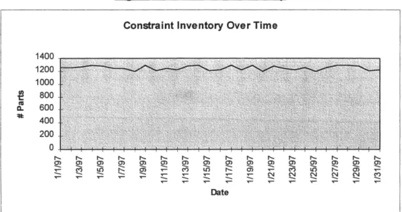
With the understanding that WIP should be needed at the constraint only and should be minimized at all other locations, I will discuss a methodology for reducing a plant's WIP. Once I questioned if inventory is truly protecting the constraint from starving, I found the two main ways to reduce WIP are through process flexibility and reliability. One tool which can be used to determine where to have the largest impact is an inventory vs. time graph at each constraint. Figure 8 contains an example of a

constraint inventory vs. time graph. The X axis is time and the Y axis is inventory level. A flat line indicates a constant level of inventory at the constraint, whereas a jagged line indicates a highly variable inventory level at the constraint.

Figure 8 -- Constraint Inventory Over Time

Constraint Inventory Over Time

1600 1400 1200 t! 1000 ~ 800 tL 600 =It 400 200 0

I'- I'-

I'-~ ~ _~

... _£2

-... ... ...

I'- I'- I'- I'- I'- r-... I'- I'- I'- I'- I'- I'-

I'-~ ~ ~ ~ _{~ ~ a5} ~ _{~ ~ ~} ~ ~

t:: ~ ... C"') ... (J) ...

... ... ... ... ... _{~ ~ ~ ~ ~ £2}

... ... _...

-

-

-

- -

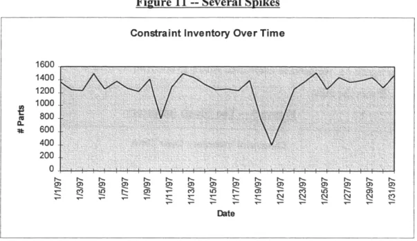
Keeping in mind that the reason for holding inventory is to protect the constraint, we can see the effect that reducing inventory will have on the manufacturing system. Any sudden drops in inventory, or spikes inthe graph, represent problems in our

manufacturing system (rocks). These spikes are of varying depth and therefore we need different levels of inventory to mitigate them. If the graph is relatively flat as in Figure 9,

the plant is carrying too much inventory and can reduce it without having any effect on throughput. If the graph reaches zero often as in Figure 10, the plant is carrying too little inventory and can increase throughput by increasing WIP. If the graph has several spikes such as in figure 11, we need to determine where to concentrate efforts to reduce

inventory levels the most.

Figure 9 -- Too Much Inventory

Constraint Inventory Over Time

1400 1200 1000 ~ 800 ClS 600 a.. :JI: 400 200 0 l""- f'-- l""- f'-- f'-- l""- f'--Q? _~ ~ m ~ Q? Q? T'"" _t?

t:

-

-

- -

-

Figure 10 -- Not Enough Inventory

Constraint Inventory Over Time

1600 1400 1200 ~_C'lI 1000₈₀₀ a.. 600 :JI: 400 200 0 f'-- f'-- f'-- l""- f'-- f'-- f'--m m ~ ~ m m ~ ;:: _{~ ~} ;::

-

- - -

Figure 11 -- Several Spikes

Constraint Inventory Over Time

1600 1400 1200 ~_l'IS 1000₈₀₀ ~ ~ 600 400 200 0 ,... ,... ,... ,... ,... ,... ,... ,... ,... ,... ,... ,... ,... ,... ,... ,... ~ m _{~ ~} ~ ~ _~ ~ ~ _~ ~ 0') m ~ m _~ ... _{~ !!? t:::} ... LO ,... ... M in en ...

-

- - -

-

-

In short, efforts should be concentrated on the largest spike. Itis important to determine the cause (or causes) of each of the spikes in inventory. Keeping in mind that we have WIP in order to keep our constraint from starving, eliminating the cause (or causes) for the largest spike allows us to reduce WIP without any adverse effects on throughput. Additionally, if we eliminate the cause for any other spike, we cannot reduce WIP for we need it to mitigate the effects of the largest spike. Manufacturing facilities should engage in the continuous process of determining the cause of the largest spike, eliminating it, and reducing the WIP levels. In doing so, the facility may find that a combination of factors has caused the spike. If this is the case, the factor contributing the largest portion to the spike is compared to the single factor causing the largest spike and that causing more inventory loss should be eliminated. By analyzing inventory at the constraint, plants can eliminate the rocks (problems) in their streams without going through the pain of hitting them.

4.2.1 Batch Processes

One cause of spikes in the Tim's inventory levels is batch processing. Some batch processes are technology imposed such as metal softening and others are self

imposed such as large batch sizes at surface preparation. It is important to understand the cause of batching in order to become a more flexible manufacturing facility. In order to minimize the amount of self imposed batching, people need to continuously question the reason for batching and work on ways to reduce the needs in the every day process. On the other hand, minimizing technology imposed batching should be addressed in the capital purchasing stage. For example, reducing the needs for batching at the surface preparation can be addressed by focusing efforts on reducing the disruptiveness of daily load/unload of the surface preparation solution baths on the surface prep process whereas reducing metal softening batching requires the use of a greater number of smaller cooling chambers rather than a smaller number of larger ones or an improvement in metal treating technology.

4.2.1.1 Costs of Batch Processes

When analyzing the cost of a batch process, it is important to know if the batch process is the cause of the largest spike in the constraint inventory chart. If it is, we can calculate the cost of holding inventory for that batch process. We do this by calculating the difference between the largest spike and the next largest one. This difference is the

amount of inventory the plant must hold to mitigate the batching effect associated with this process. We can multiply this amount of inventory by the cost of holding inventory to get a cost for batch processing. It is important to realize that if a particular process is

not the cause of the largest spike, the plant cannot reduce inventory at all by eliminating batching in this particular process. Eliminating the largest spike is the only way to reduce inventory levels and still maintain the same constraint protection.

In addition to the economic value associated with the cost of tied up capital, there is a strategic and quality value to reducing inventory. Although these two values are much more difficult (or even impossible) to accurately calculate, they must be addressed.

Determining a strategic value to flexible manufacturing is a task combining