The design and implementation of a portable data acquisition system

by

Thomas Deng

Submitted to the Department of Electrical Engineering and Computer Science

in Partial Fulfillment of the Requirements for the Degrees of

Bachelor of Science in Electrical Science and Engineering

and Master of Engineering in Electrical Engineering and Computer Science

at the Massachusetts Institute of Technology

Hi

May 1994

,'-

n

..

rOF TECHNOL.)CYY

AtAC;rUSETTS 1HS1-iI UaTE

Copyright 1995 Thomas Deng. All rights reserved.

JAN 2 9 1996

LIBRARIES

The author hereby grants to M.I.T. permission to reproduce

and to distribute copies of this thesis document in whole or in part,

and to grant others the right to do so.

Author

De-Artment of Electric Engineering and

~

by

/Certified

(\

l

-

/-.

Certified

by

(oh,5~

,,~

L

. , A_ ,

X__

Accepted

by

! i

.* f

-B

-

.

II

1

-Chairman, Department Committe o:

Computer Science May 18, 1995

George W. Pratt

Thesis Supervisor

F.R. Morgenthaler

n Graduate Theses .

The Design and Implementation of a Portable Data Acquisition System

by

Thomas Deng

Submitted to the

Department of Electrical Engineering and Computer Science

May 18, 1995

In Partial Fulfillment of the Requirements for the Degrees of

Bachelor of Science in Electrical Science and Engineering

and Master of Engineering in Electrical Engineering and Computer Science

ABSTRACT

The portable data acquisition system provides a way for a person with minimal technical background to sample and analyze impact data for various running surfaces. The system allows the the user to sample and store input data from an accelerometer. After the data is acquired, the system calculates velocity and displacement curves, which are then used in a non-linear damped spring model to determine loss and stiffness characteristics for the impacted surface. The graphical user interface and the developed suite of tools that drive the data analysis engine can readily be adapted to a variety of applications.

Thesis Supervisor: George W. Pratt Title: Professor of Electrical Engineering

Table of Contents

Table of Contents ...

3

List of Figures ...

... ...

5...

List of Tables ...

6

1. Introduction ...

7

1.1. Background ... ... ... ... 7 1.2. Objective... 8 2. Impact Analysis ... 8 3. Design Overview ... 9 4. System Hardware ... 10

4.1. Data Acquisition Hardware .

.

.

...

10

4.1.1. Signal Acquisition ... 10

4.1.2. Signal Conditioning ... ...

11

4.1.2.1. Signal Amplification/Attenuation ... 11

4.1.2.2. Noise Filtering ...

11

4.1.3. Data Sampling ... 12

4.1.4. Data Storage ...

...

12

4.2. Laptop System Requirements ... 12

5. System Software... 13

5.1. Programming Methodology

..

..

...

13

5.2. Microsoft Visual Basic ... 13

5.2.1. Microsoft Visual Basic Selection ... 13

5.2.1.1. Portability ... ... 13

5.2.1.2. Adaptability ... 14

5.2.1.3. Programmability ... 14

5.2.1.4. Comprehensibility ... 14

5.2.2. Introduction to Microsoft Visual Basic ... 14

5.2.2.1. Forms, Controls, and Event-Driven Messaging ... 14

5.2.2.2. Object-Oriented Programming and Code Modules ... 15

5.3. Graphical User Interface ... . 15

5.3.1. Common Dialog Form (frmCDlog) ... 15

5.3.2. File Input/Output Test Form (frmCheckFiles) ... 16

5.3.3. Main Program Form (frmMain) . ... ... 17

5.3.4. Show Status Form (frmStatus)

... 18

5.3.5. Data Acquisition Configuration Form (frmConfig) ... 19

5.3.7. Data Plot Form (frmGraphl)

... 20

5.3.8. Set Graphing Range Form (frmRange) ... 21

5.3.9. Display Results Form (frmResults) ...

... 22

22...

5.4. Data Acquisition ... 23

5.5. Data Analysis ...

... ...

...

... 24

5.5.1. Data Processing ...

24

5.5.1.1. Data Filtering ...

...

24

5.5.1.2. Data Conversion

.

...

24

5.5.1.3. Integration ...

...

24

5.5.1.3.1. Trapezoidal Method ... 24

5.5.1.3.2. Constants of Integration ...

25

5.5.1.4. Non-Linear Damped Spring Model ... 25

5.5.2. Data Display ...

...

... 26

5.5.2.1. Setting Default Ranges ... 26

5.5.2.2. Checking for Valid Ranges ...

...

2...

26

5.5.2.3. Setting User-Defined Ranges . ... 26

5.5.2.4. Zooming ...

...

27

5.5.2.5. Plotting a Grid ... 27 5.5.2.6. Showing Coordinates .. ... 27 5.6. File H andling ... 27 5.6.1. File Types ... ... ... 27

5.6.2. File Functions ...

...

27

6. Using the Impact Analysis System ... 28

6.1. Installing the Impact Analysis System ... 28

6.2. Running a Characterization Trial ... 28

6.3. Manipulating Graphs ... 28

6.4. Saving and Retrieving Data ... ... 29

7. Sample Impact Analysis Trial . ... 29

7.1. Data Acquisition Configuration ...

... 29

7.2. Results ...

...

...

.

...

29

8. Expandability and Adaptability .. ... ... 31

8.1. Impact Analysis . ... 31

8.2. Other Applications ...

...

31

9. Conclusions ... ... ... . ...32

Bibliography... ... 33

FRM CONFI.FRM (frm Config) ... 39

FRM DATA.FRM (frm Data)...4... 44

FRM GRAPH .FRM (frm G raphl) ... ... 46

FRM M A IN.FRM (fim M ain) ... ... 48

FRM RAN GE.FRM (frm Range) ... 60

FRM RESULT.FRM (frm Results) ... 67

FRM STATU.FRM (frmStatus) ... 68

Appendix B: Code ... 70

DAQ.BAS ...

71

GRAPH ICS.BA S ... 74

IOFUN C.BA S ...

95

M AIN .BAS ... 104

PRO CESS.BA S ...

122

WDAQ_

VB.BAS ...

130

List of Figures

Figure 1: System Functional Block Diagram ... 10

Figure 2: Sample Plots for an Impact Analysis Trial ... 11

Figure 4: Windows Standard Dialog Box ... 17

Figure 5: M ain Program Form ... 18

Figure 6: Status Dialog Box ... 20

Figure 7: Data Acquisition Configuration Dialog Box ...

...

... 20

Figure 8: Data M atrix Display Form ... 21

Figure 9: Data Plot Form ...

22

Figure 10: Range Dialog Box ... 23

Figure 11: Results Form ... 24

Table 1: Main Menu Item Description ... 18 Table 2: Results from Sample Impact Analysis Trial ... 32

1. Introduction

1.1. Background

Recent technological advances have allowed for the development of electronic devices which are smaller and more powerful than ever. These enhanced capabilities have led to a corresponding shift in the engineering paradigm towards portable onsite

computing. Laptop computers and the wide array of available PCMCIA expansion cards

provide the computing power and application flexibility required. Increasingly lower

power consumption, longer battery life, lower component prices, and better computational

power, as well as heightened networking capabilities, help drive the revolution towards mobile computing, and there remain fewer and fewer reasons to remain tied to a laboratory or central computational facility. Data can now be collected efficiently in the field and analyzed easily on the spot for such diverse applications as geological surveys or biophysical studies.

Traditionally, the field data required for such analyses could be obtained only by using expensive and cumbersome electronic equipment. Operating this equipment required a nontrivial amount of technical expertise, and because such systems did not generally have a standardized user-friendly interface, a significant amount of training was

often required. Furthermore, after the data was acquired, it had to be ported to a

computer system back in the laboratory where it could be analyzed. Problems with the acquisition equipment would not be detected until the data reached the lab, in which case

it could take weeks or months to handle the logistics of arranging to acquire new data.

In addition to the problems presented by the acquisition equipment, the analysis system was both expensive and not relatively accessible. Even under normal

circumstances, it would not be uncommon for several weeks to pass before the end user

received the computer analysis, which would often be too abstruse to offer the end user

much valuable insight.

With a portable data acquisition system, data could be acquired and analyzed within seconds of a sample run. The entire system would be self-contained, with no additional unwieldy equipment necessary. Problems with the signal acquisition equipment

would be detected immediately and could be corrected on the spot.

Using an

implementation based on a laptop computer and a PCMCIA data acquisition card would be comparably inexpensive and extremely portable. Finally, with the development of appropriate application software with a user-friendly interface, there would be no reason why an end user with minimal technical background could not operate the system and gain immediate and accurate feedback in a useful form from the resulting analysis.

1.2.

Objective

With this motivation in mind, the primary objective of this thesis will be to develop

a set of software tools to exploit the capabilities of a laptop-based portable data

acquisition system. Although these tools will be easily adaptable to the needs of a variety

of applications, the particular application for which these tools will be tailored is the

analysis of impacts on various track surfaces.

2.

Impact Analysis

The field of impact analysis is particularly well suited to the development and testing of a data acquisition system for several reasons. First, there are several well-understood models that have been developed for analyzing impacts. Second, the forces that characterize an impact can be determined readily by using an accelerometer as the input to the system. Finally, there are many applications for a portable impact analysis system.

The motivation for gearing the impact analysis system specifically towards studying the characteristics of tracks is twofold, since both track speed and safety could be optimized. Intuitively, one would consider harder tracks to be faster, since less energy is dissipated in the impacts on the track. For the same reason, harder tracks could be

considered less safe than tracks with more resiliency. It would seem, therefore, that track

design necessarily involve a tradeoff between speed and safety concerns.

However, McMahon and Greene [1,2] discovered that by modeling a track as a non-linear damped spring with a characteristic natural frequency and matching this frequency with the corresponding frequency of a runner, tracks could be designed which

were up to 3% faster than traditionally designed tracks. In addition to being faster, these

tracks would be more compliant than the traditional tracks, which would lead to an increased degree of safety and comfort.

Track safety is arguably even more crucial for horse racing. Each racehorse

represents a tremendous investment for his/her owner, and safety for the racehorse during

both races and training is a major concern from both a financial and a humanitarian perspective. A portable impact analysis system could be used to quickly and easily determine the relative safety of a variety of racetracks.

Therefore, the system could be used both in the design of safe, fast tracks, as well as in the analysis and characterization of existing tracks.

3. Design Overview

The design and implementation of the system can be divided into three functional blocks, as depicted in Figure 1. The interface is used to obtain user-defined parameters and to present results to the user in a meaningful form. The data acquisition module

performs the sampling and the storing of the data, and the data analysis module processes

and formats the data for easy interpretation.

Figure 1: System Functional Block Diagram

For example, a typical track characterization may take the following form: First, the user initializes the system, either using a set of default parameters or customizing the

parameters. The user would then drop a hammer fitted with an accelerometer onto the

track surface. The impact would trigger the acquisition module, which would store the

sampled acceleration data. From this data, corresponding velocity and displacement data would be generated, and characteristics of the impact could be extrapolated. Figure 2

shows sample results for one typical trial.

User Interface

Data

Acquisition

Data Acquisition

Data Analysis

I

Figure 2: Sample Plots for an Impact Analysis Trial

4.

System Hardware

The system hardware has two main functions. First, the data

provides the system with the data. Second, the laptop computing

capability for data analysis and user interface.

acquisition hardware system provides the

4.1. Data Acquisition Hardware

The data acquisition hardware has four components: 1) signal acquisition, 2) signal conditioning, 3) data sampling, and 4) data storage.

4.1.1. Signal Acquisition

For a general data acquisition system, the analog voltage input would be generated by a transducer in response to a physical phenomenon. For instance, a thermistor could be

used to measure temperature change, a strain gauge to determine force on an object, or a

microphone to characterize acoustic waves. The range of the transducer's output voltage

levels would not be constrained by the overall system, since the signal could be attenuated or amplified to the desired range.

JEile Sample nalyze Graph .1~ndow Help

A'i ' "~ f''"'""""''~ -'- ' ":l::ii-i" i. Displacement t* vs. Time ::. Stiffness vs. Time - I

.005

60-.i

' .5 i

t

1 1.5 f2

.

Aso

.

5 -2 -.005 -4-.01 -.015, -50

Velocity vs. Time I i Loss vs. Time Results

4000 Threshold: -.6157

_impact 121

.1 tokeoff: .187

3000. Impact Duration: .007

mpact Rise Time: .03 .05 2iVelocity at Impact .098263

Energy at Impad: .004820

elocity at Takeoff- -. 079:39

sO~~~ . , ' . } 1 E~~~~~~~~nergy at Takeoff: 003187

.1 .2

/

1000 nergy Absorbed during Impact -.001641

t

/~verage

Loss: 2012.144

Pek Loss; 3273.137

.1 .2 .3 verage Stiffness: 6.15436

The test framework for the transducer could range from extremely elaborate

mechanisms to relatively simple devices. For example, a heating mechanism may be used to heat or cool an object whose temperature change would be measured by the thermistor;

a tank fitted with a rowing framework could have strain gauges attached to the oarlocks

to measure forces on the oar; or an ultrasound system could be used to broadcast acoustic waves through a material into a microphone to determine the characteristics of that material.

For the impact analysis system, the signal acquisition mechanism uses an accelerometer based on a piezoelectric cantilever beam, which is attached to a hammer designed to isolate acceleration to one dimension. The accelerometer used generates an

analog voltage output calibrated 10 mV/G, where G is the Earth's gravitational constant

(9.8 m/s2 or 32 ft/s2).

4.1.2. Signal Conditioning

After the transducer signal is produced, signal conditioning may be required to

amplify/attenuate the voltage ranges to the desired levels or to filter out any associated

noise.

4.1.2.1. Signal Amplification/Attenuation

Because of the wide output voltage ranges for the variety of transducers that could

be used, amplification and/or attenuation of the signal may be necessary. Depending on the particular characteristics of the given transducer signal, almost any type of

amplifier/attenuator could be used that would preserve an allowable signal to noise ratio

and satisfy frequency constraints.

The accelerometer signal for the impact analysis system is amplified with a battery-powered amplifier (Bolt Beranek and Newman) which acts as a voltage follower with a gain of 10. The input to the amplifier is a single small-gauge wire connected to the

accelerometer, while the output is a coaxial cable with a two-pin connector at the other

end. A plastic tab embossed with "GND" differentiates the ground pin and the signal pin

on the connector.

4.1.2.2.

Noise Filtering

Filtering may also be necessary to condition the amplified/attenuated signal in order to improve the signal to noise ratio. This may involve using various bandpass filters to remove a DC offset from the signal or to attenuate high frequency noise. Again, the filtering methods available are numerous and virtually unconstrained. In general, however,

software filtering during the data analysis and processing phase would allow for more

flexibility than hardware filtering.

For the impact analysis system, no signal filtering in hardware is used besides the buffering of the signal amplifier.

4.1.3.

Data Sampling

Sampling is performed by a National Instruments Type II PCMCIA data acquisition card (DAQCard-700). The card is characterized as a multifunction input/output board equipped with a 12 bit ADC which has 16 single-ended or 8 differential

analog inputs.

The input voltage range is configurable for ±10 V, 5 V, or ±2.5 V, but has overvoltage protection of ±45 V. The analog signal resolution of the 12 bit ADC is 4.88 mV in the ±10 V range, and the output is automatically sign-extended to 16 bits. The maximum sampling rate is 100 kSamples/s, and the board has an internal counter/timer which can be used as the sampling interval clock at a 1 s resolution. However, an external sampling clock signal can also be provided.

For the impact analysis system, the DAQCard-700 is connected through a ribbon-cable to the DAQCard-700 I/O connector. Pin 1 on the DAQCard-700 is indicated by a white dot, while Pin 1 on the ribbon cable is indicated by an arrow impressed into the plastic. Analog ground wires were soldered to Pins 1 and 2 (AIGND) and an input wire was soldered to Pin 3 (ACHO), since the conditioned accelerometer signal requires only

one single-ended analog input channel. No other connections to the DAQCard-700 are

necessary, since the internal sampling clock is used.

The actual interface between the sampling module and the acquisition module are a pair of wires with alligator clips on the ends. These wires connect the soldered extensions

of the DAQCard-700 I/O connector to the two-pin connector of the amplifier output.

Ground on the two-pin connector is marked with a tab on which "GND" is embossed.

4.1.4.

Data Storage

The sampled data is then read into the laptop's main memory (RAM) and can be later saved to disk. The laptop running the impact analysis application should have a

minimum of 8 megabytes of RAM and at least 30 megabytes of free disk space.

4.2.

Laptop System Requirements

The laptop computer should be capable of running Microsoft Windows 3.1 and should be equipped with a Type II PCMCIA slot. The application software itself will not be demanding in terms of memory requirements, but system memory will constrain the maximum allowable size of the data array (maximum number of samples stored). As mentioned before, the system should have at least 8 megabytes of RAM and 30 megabytes of free disk space.

5.

System Software

In addition to the above hardware, software would be required to control the

interaction among the listed components, as well as to provide a user-friendly interface.

Software drivers provided by National Instruments provide a low-level interface, but the

software framework for the application should be implemented in a high-level language, preferably in an environment supporting a graphical interface.

The following description of the application software is intended only to give a

broad overview of the developed tools and the design choices that were made. An

exhaustive description of the functionality of each subroutine or function would be

redundant for three reasons: 1) the code itself is written in a highly readable programming

language, 2) the program is written in a very structured format, which should enhance readability, and 3) the comments in the body of the code serve as sufficient documentation

for the intended function and operation of each subroutine/function.

The overview will discuss the following: 1) the development methodology of the code, 2) the selection of Visual Basic as the application development language, 3) the

graphical user interface, 4) data sampling and the interface to the National Instruments

DAQCard-700, 5) data analysis methods and plotting techniques, and 6) file handling.

5.1.

Programming Methodology

The top-down design was approached in a modular fashion, with each of the tools designed with a broader perspective in mind than just the current application. This approach is consistent with the objective to build not just an impact analysis system, but to construct a suite of tools that would be readily adaptable to a variety of data acquisition applications.

Implementation and testing was undertaken modularly also, but with a bottom-up methodology. Each of the individual modules was built and tested in a stand-alone fashion

before being integrated with the rest of the tools in the application. This approach was

taken to ensure the portability and adaptability of the individual modules in the system.

5.2.

Microsoft Visual Basic

5.2.1. Microsoft Visual Basic Selection

Microsoft Visual Basic was chosen as the high-level programming language in which the tools and integrated application would be developed. Four primary reasons justify this choice: 1) portability, 2) adaptability, 3) programmability, and 4)

comprehensibility.

Although the development of the Visual Basic tools supports a library-oriented design methodology, the capability of Visual Basic to synthesize all the necessary library files into an executable file was very attractive, since this would facilitate the distribution of the application software.

5.2.1.2. Adaptability

Visual Basic's support of library-oriented development and object-oriented

programming was consistent with the objective of developing a set of tools that could be

adapted for use in other data acquisition applications. In addition, Visual Basic's event-driven messaging capabilities are supported by the data acquisition function library developed by National Instruments.

5.2.1.3. Programmability

A straightforward user interface was required so that an untrained user could easily operate the system and obtain the needed information quickly. A graphical user interface is therefore ideal for this application. Every effort was taken to make the appearance and function of the application consistent with standard Windows applications, including the menu-driven interface and multiple-document interface (MDI). In this manner, the application interface was designed for an intuitive look and feel that would be attractive and non-intimidating even for inexperienced computer users.

The desire to create a user-friendly graphical interface for the application was fulfilled by Visual Basic's use of forms. By using these forms, with their set of defined controls, a graphical user interface was easy to construct. In addition, library-oriented, object-oriented programming in Visual Basic supported the modular design and

implementation methodologies that were key to programmability.

5.2.1.4.

Comprehensibility

Finally, these features not only made Visual Basic attractive from a programmer's perspective, they also enhanced the readability and comprehensability of the code. Even someone with limited programming experience would be able to easily adapt the tools for his/her own data acquisition application.

5.2.2. Introduction to Microsoft Visual Basic

Microsoft Visual Basic is based on the familiar BASIC programming language,

which was designed to make programming as intuitive as possible. The biggest difference between Visual Basic and conventional BASIC is Visual Basic's use of forms, controls, and event-driven messaging, which makes the creation of a graphical user interface relatively simple. In addition, Visual Basic's support of object-oriented programming and individual code modules makes program flow easy to follow.

Visual Basic forms provide the tool set from which the familiar window/dialog box

interface is constructed. A variety of different controls can be placed on each form,

including list boxes, command buttons, option buttons, picture boxes, text boxes, and

scroll bars. With conventional programming tools, each window and control would have to be individually coded into the body of the application. Visual Basic, however, provides a graphic form editor which allows the application designer to custom tailor the form and its controls. In addition, code is automatically attached to each form and its controls

which generate events corresponding to user actions. For instance, when the user moves

the mouse on a form, a Mouse_Move event is generated. Similar events are generated for

other mouse operations, command button clicks, text box changes, etc.

In conventional BASIC, program flow is largely sequential, even with the use of subroutines and conditionals. With the additional power and flexibility event-driven messaging provides, Microsoft Visual Basic allows the developer to give the user much more control over program flow. With this capability, a much more intuitive graphical user interface can be created with Visual Basic than the traditional text menu interface

common in conventional BASIC.

5.2.2.2.

Object-Oriented Programming and Code Modules

In addition to providing tools for constructing a graphical user interface, Microsoft

Visual Basic also facilitates application development by treating forms and controls as objects, each with its own set of attached attributes, which are either properties or

methods. Using linked attributes (object-oriented programming) reduces the complexity

of application code by several orders, since the linking and updating is done automatically. This contributes to relative ease in development and in program comprehensibility.

Achieving these goals are also aided by Visual Basic's support of development modularity. Each code module has a section where general variable declarations can be made. Although Visual Basic supports variable definition by context, using explicit

variable declaration makes the code more readable. The use of stand-alone code modules

is also consistent with the objective of producing a library of procedures and functions from which additional data acquisition applications can easily be generated.

5.3. Graphical User Interface

The graphical user interface for the impact analysis system consists of nine forms,

which are described below.

5.3.1. Common Dialog Form (frmCDlog)

This form is always hidden because the two custom controls on the form, the

Common Dialog custom control and the National Instruments Analog Trigger custom

control never need to be visible. The only reason there is a separate form for these two controls is that the main form is an MDI (Multiple-Document Interface) form, which does

not allow custom controls to be placed on it.

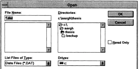
The Common Dialog custom control itself is used for generating several

Windows-standard dialog boxes (Figure 4), including Open File, Save File, Save As, and Print. Although the control offered much more functionality than was used, incorporating these

standard dialog boxes into the integrated application was consistent with the goal of

providing a standard Windows look and feel for the application.

i.-1-

.1 .-.-_-_-- F e ... .. : -::~~~·2::::·5··: ... .-..: : :: ..-... :... ,:... :::::::::::. ... '. .- .a,

File Name: Directories: _{I'.'i~l ·iiiiiiiii?~ :'ii!i iiii'i}

Lis..Files of

T~jrp.-rList Files of Type:

c:\aarghthesis

; c:l

b

aargh

b

thesis

.tf backup Drives:

l

Blead Only

IDate Files r.DAT)

I

N c : I

.::-.:. ::.: .: :.:.: :%::::: :-.·~:. .:.:.: .:.:~:~-. : .: .--. ~-.-.--..,-...-- :::..-.-..-:.... ...

:~-.~:~;~:.-Figure 4: Windows Standard Dialog Box

The National Instruments Analog Trigger custom control ties the National

Instruments data acquisition device drivers to Visual Basic's high-level event-driven messaging capabilities. The Analog Trigger fires only when the signal passes through a

specified window and crosses a specified threshold, at which point an event is generated and passed back to the Visual Basic environment, where the event can be used to trigger

other program actions.

5.3.2. File Input/Output Test Form (frmCheckFiles)

This form is used only as a testbed for the file input/output functions for both

sequential files and binary files (described in Section 5.6 File Handling). As each entry of the specified file is read into main memory, it is also appended to the entry in the given text box. The two text boxes allow the contents of two files, a sequential file and a binary file, to be compared.

5.3.3.

Main Program Form (frmMain)

I

I

The Main Program Form (Figure 5) serves as the primary interface form for the impact analysis application. The menu-driven interface is incorporated into this form, and the various menu items are delineated in Table 1.

File Sample .::::::: :: .. 1 Window Help:::

Figure 5: Main Program Form

Table 1: Main Menu Item Description

Menu Item Function

File Open

Binary reads data from binary file

Text reads data from sequential file

Close clears data in memory

Save As

Binary saves data into binary file

Text saves data into sequential file

Print

All Forms prints all forms Sample

Run starts data acquisition

Configuration... allows user to define data acquisition parameters

Analyze

Show Data tabulates data in memory

Process Data processes the raw acceleration data

Prepare Graphs prepares and displays data plots

Graph ___

Line connects data points

Grid plots a grid on the graph

Coordinates displays coordinates of cursor position

Zoom In allows user to zoom into a user-defined window

Zoom Out displays full graph

Replot redraws data plot

Scale allows user to manually define plot ranges

Window

Cascade arranges windows in cascade fashion

Tile Horizontal tiles windows horizontally

Tile Vertical tiles windows vertically

Arrange Icons arranges iconified windows

Help displays help awindow

5.3.4.

Show Status Form (frmStatus)

An important part of the graphical user interface is to keep the user involved at all

times, even at points when the processor is busy. Otherwise, with no feedback, a lengthy

computation or process could cause the user to believe that the application has crashed.

Therefore, besides the status bar on the main form, a Show Status Form (Figure 6) is provided which is activated during longer periods of latency, such as during file operations and initial data processing.

* .*.*...;...~:~i~:~:~:~;:

~

* :xxm *. t

1200 of 2000

Figure 6: Status Dialog Box

5.3.5.

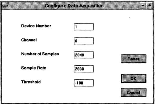
Data Acquisition Configuration Form (frmConfig)

The Data Acquisition Configuration Form (Figure 7) allows the user to specify

several parameters for the actual sampling of the data. These parameters are later passed

to the National Instruments device drivers through the data acquisition function calls.

This form is accessed through the main menu on the main form under Sample -> Configuration. Five parameters can be specified: 1) the device number of the PCMCIA data acquisition card, as set in the Windows card configuration utility, 2) the channel on the PCMCIA card which the input analog signal is driving, 3) the desired number of samples, 4) the desired sampling rate, and 5) the threshold signal level at which the system should trigger. The default values for the above parameters are held in the Tag fields of

the respective text boxes.

Device Number 1 Channel Number of Samples 2048 Sample Rate 2000

Threshold-100

[-1 O0~~

5.3.6.

Data Matrix Display Form (frmData)

Figure 7: Data Acquisition Configuration Dialog Box

·51·II·'·'·f·:·'·:·Sf·.:·:C··5:

iil::::::.:..ii::::R::::::: 55'22·'·';·"::::::::5·· ::;:;X::::::::·:S·:·:;X ·_{,tc·fil '" ';2·':::::,:::1:::1::::::':':': , c.:::::::::::::iiii:::I:::::} . : :.·.·2.:.::;::·:·:·:Ss·.. _{·:· :} s ;:;:·1··:':::::::::.:"..:;:.n, W :::j s·;·;··::;:;:;:;:;::::: iiii Lf t:·:fX;I:::::::SY... ;:;:;:·:;:;·;·C·-·5::::: :::::::'''':.:5.::::..'; S5...s 5···i ·· 2·51

A data matrix display form (Figure 8) was provided for two reasons. First, for

debugging and testing purposes, some method was required to be able to see all the

information that was in the data array, included measured and calculated values. Second,

the data display form allows the end user to get more detail about specific data points, if

sufficiently detailed information is not readily discernible from the data plot.

Eie Sample Analyze QGraph AIndow elp

.. . I

t, j~ I'- ~, A, 4 !~.- i. Velocity vs. Loss vs.

Acceleration isplacementArlnessvs. Results Time Time vs. Time vs. Time Time

Figure 8: Data Matrix Display Form

5.3.7.

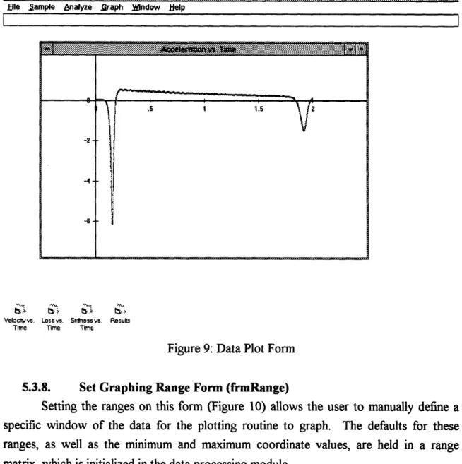
Data Plot Form (frmGraphl)

The graphs of the data series contained in the data matrix are plotted on the Data

Plot form (Figure 9). This form exploits the capabilities of the Multiple Document

Interface (MDI) and Visual Basic's object-oriented support by using an array of instances

of the Data Plot Form. This approach facilitated programming, since creating a new form

for each of the data series would have been tiresome. In addition, the array of Data Plot

Form instances corresponded to each of the data series stored in the data matrix, so rather

than having to write plot programs separately for each series, only one plot routine had to be implemented.

Jima Aelerntion Yeloci D DnlammeaI na stiflmess

.0002 -.02563 .018279 -.000235 0 0 .0004 -.02626 .018274 -.000232 2.103212 1.463707 .0006 -. 02626 .018269 -.000228 -173.4878 .7289092 .0008 -.02563 .018263 -.000224 2.004265 1 427991 o001 -.02563 .018258 -.000221 2.004034 1.427998 .0012 -. 02563 .01 853 -.000217 2.005411 1.428005 .0014 -.02563 .018248 -.000214 -170.7284 -.593083 .0016 -.02501 .018243 -.00021 174.6444 3.380021 .0018 -.02563 .018238 -.000206 2.007097 1.428014 .002 -.02563 .018233 -.000203 2.007575 1.428021 .0022 -.02563 .018228 -.0001 99 2.008245 1 .420027 .0024 -.02563 .018222 -.000195 177.6017 3.309734 .0026 -.02626 .018217 -.000192 2.109704 1 463682 .0028 -.02626 .018212 -.000188 2.11108 1.463696 .003 -.02626 .018207 -.000184 -173.4855 -.314263 .0032 -.02563 .010202 -.00101 2.011195 10034 42863 0196 00077 .0034 -.02563 .018196 -.000177 177.6077

Ble Sample nalyze raph WIndow Help I L Velocityvs Time Loss vs. Time i'~y.e v. Shtfness vs. Results Time

Figure 9: Data Plot Form

5.3.8.

Set Graphing Range Form (frmRange)

Setting the ranges on this form (Figure 10) allows the user to manually define a

specific window of the data for the plotting routine to graph. The defaults for these

ranges, as well as the minimum and maximum coordinate values, are held in a range matrix, which is initialized in the data processing module.

~~~s~

s~~·~~~2~s~

. ....

.. .. ...

...

s....ss....

J

Figure 10: Range Dialog Box

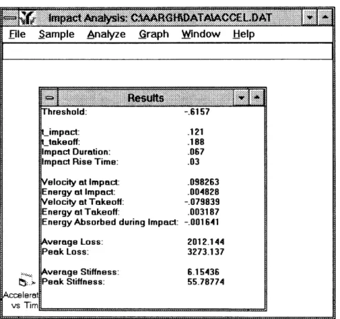
5.3.9. Display Results Form (frmResults)

Statistics of particular interest are calculated during the data analysis segment of

the code, and the Display Results Form (Figure 11) provides the medium for these final

results to be communicated to the user. Such information as impact time, rise time, peak acceleration, initial and final velocities, initial and final energies, etc. are summarized on this form. Minimum X -05 MaxIwmumX: 125 Minimum Y: 9467 047336

I

15 :~:::::~~::~:::

~:~:~w

· ;·;~;;:i.ss.s·:: ;e

~

..,M;:~.:~:.:::ss·:S:~::::~ii~:: f... ·· ' · i

~S

::::x··::~::~;~:~::~:::

~siwF·;·;:::::::'5'·

· ·

~:~":.0::.n

:::2··~· ... ...

ii~~i~i: i:. iii8 ... :~~::::: _--- - --- --- ...ji· ...

·:X: i:~::~::i::::::·... . :::::: ':i'xww:·.:·.::::

File Sample Analyze Graph Window Help

I Accelerat vs Tim Threshold: - 6157i Threshold: -.6157 Limpact: .121 _ takeoff: .188 Impact Duration: .067

Impact Rise Time: .03

Velocity at Impact: .098263

Energy at Impact: .004828

Velocity at Takeoff: -.079839

Energy at Takeoff: .003187 Energy Absorbed during Impact: -. 001641 Average Loss: 2012.144 Peak Loss: 3273.137 Average Stiffness: 6.15436

Peak Stiffness: 55.78774

,...

Figure 11: Results Form

5.4. Data Acquisition

Data sampling is achieved simply through the use of the dynamic linked library (DLL) provided by National Instruments (NIDAQ.DLL). A set of useful function calls are defined specifically for Visual Basic, which is extremely helpful in keeping the programming at a high level of abstraction. The data acquisition routines that are required are contained in (DAQ.BAS), and the National Instruments declared functions are contained in (WDAQ_VB.BAS).

As mentioned previously, five parameters are needed to characterize a data acquisition run: 1) the PCMCIA device number, 2) the analog input channel , 3) the number of samples to be acquired, 4) the desired sampling rate, and 5) the threshold signal level. These five parameters are used to initialize two GeneralDAQEvent controls which generate events when certain conditions are fulfilled. GeneralDAQEventl is configured to trigger when half of the desired number of samples are acquired, while

GeneralDAQEvent2 .triggers when the sampled signal passes through the threshold.

In order to run the acquisition continuously until the trigger conditions are met, the double-buffering mechanism provided by National Instruments is used in conjunction with

National Instruments' memory management functions. Both mechanisms are discussed in

detail in the National Instruments Function Reference.

5.5. Data Analysis

Data analysis for the impact analysis system consists of two components. First, the

sampled data needs to processed in order to extract useful information. After the data

processing is completed, the results need to be presented back to the user in a clear and concise format.

5.5.1.

Data Processing

The bulk of the data processing for the impact analysis system takes place in PROCESS.BAS. The key steps in the processing of impact data are: 1) filtering the sampled data, 2) converting the data to acceleration units, 3) integrating the acceleration data to obtain velocity and displacement data, and 4) using the non-linear damped spring model to determine loss and stiffness data.

5.5.1.1.

Data Filtering

Only rudimentary data filtering techniques were implemented, such as compensating for offsets and performing a moving average on the data. In the final impact analysis system, only offset compensation was required.

5.5.1.2. Data Conversion

As mentioned before, the output of the data acquisition hardware was an analog

voltage signal scaled to 10 millivolts per one unit of Earth's gravitational acceleration (10 mV/G). In addition, to make the information more intuitive, positive acceleration was redefined to be down, whereas the original data had positive acceleration defined to be up.

5.5.1.3.

Integration

After the acceleration data is calculated, it is integrated twice; once to obtain velocity data, and once for displacement.

Two methods of integrating were considered. First, a curve fit could be used to

determine an expression for the raw data, and that expression could be used for the integration. The alternative was to use a numerical integration technique. The first method was attractive because of the existence of models which give empirically derived

equations for acceleration in an impact, which would help in curve-fitting. In addition, numerically integrating the acceleration data would still leave the problem of determining

constants of integration. Despite these factors, the second method was chosen because it

was more adaptable to other applications, and would therefore be more consistent with the

stated overall objective.

Numerical integration was done using the trapezoidal method, with no set time

increment, but rather calculating the time increment for each step. The error inherent in using this integration technique should be negligible compared to the sampling error.

5.5.1.3.2. Constants of Integration

The constant for the first integration is determined by using the time of flight

between the first and second impacts of the hammer. From this time of flight, the takeoff

velocity from the first impact can be calculated and reconciled with the corresponding value from the numerical integration.. The constant for the second integration is determined by setting the displacement equal to zero at the point where acceleration crosses the zero axis, representing physically the time at which the hammer contacts the

track surface.

5.5.1.4.

Non-Linear Damped Spring Model

The linear constant coefficient differential equation for a linear damped spring is

Ma + av+ kx =0

where M is mass, ax is loss, k is stiffness, a is acceleration, v is velocity, and x is displacement. The nonlinear damped spring model differs from this only in that the loss and stiffness coefficients are not constant and instead vary with time. Track characterization using this model was investigated by McMahon and Greene, and their work shows that the model is accurately descriptive.

In order to determine the loss and stiffness coefficients at each point in time for the track being characterized, a numerical method is used. The assumption is that the loss and stiffness coefficients for two adjacent sample points do not vary excessively, so for each

two adjacent sample points, the corresponding two equations for the nonlinear damped

spring model are solved for the loss and stiffness coefficients. The resulting expression for the loss at each point is

a = -M xi +

l

_-

1

ai

V. Xi i- + xi

k=MVi+lai

1

_Vi-lai

V-i lXi+1

i+ lxi-i

5.5.2. Data Display

As mentioned before, three forms are used to give the user feedback about the

analyzed data. First, all the data can be viewed using the Analyze -> Show Data menu command. Second, a synopsis of the calculated characteristics of the impact is tabulated automatically on the Display Results Form. Finally, each of the five calculated curves (acceleration, velocity, displacement, stiffness and loss) are plotted on Data Plot Forms.

The code responsible for generating and manipulating the data plots for the

application was the most complex in the application. The preparation of the data plots, including the initial definition of the range matrix and the actual plotting of the data, is handled by the code in GRAPHICS.BAS, as could be expected. However, plot manipulations were triggered by events generated by selections from the main menu, as

well as mouse operations on the actual Data Plot Forms (FRMGRAPH1.BAS), A lot of

functionality was implemented, all of which may not be exploited in the impact analysis system. However, the comprehensiveness of the graphics tool set makes it especially useful in the development of other applications. The graphics functions implemented are described below.

5.5.2.1. Setting Default Ranges

The default ranges of the data plots are set by finding the first acceleration peak and centering that in the plot. These default ranges are then stored in the range matrix,

where the user can revert to at will. Also, the plotting routine will revert to the default

when the user defines an invalid plot range.

5.5.2.2. Checking for Valid Ranges

During data processing, each of the data series is searched through to find

minimum and maximum values. These extrema are stored in the range matrix, and when the user defines a custom range, these values are checked to ensure that the user-specified

data plot window lies within the data range.

5.5.2.3.

Setting User-Defined Ranges

As mentioned before, the Set Range dialog box can be used to manually enter the minimum and maximum coordinates for the plot routine to use. The user-defined ranges are then checked to ensure their validity (see Section 5.5.2.2). If the defined range is

valid, the data in the active window is replotted using this scale, and if the defined range is invalid, the application reverts to the default range as defined in Section 5.5.2.1.

5.5.2.4.

Zooming

In addition to manually setting the plot range using the Set Range dialog box, the user can zoom into a certain region of the current plot by selecting Graph -> Zoom In on the main menu and then drawing a zoom box on the current graph. Again, the new ranges that would be defined by zooming in are checked for validity before they are used (see

Section 5.5.2.2).

Zooming out allows the user to display the entire range of acquired data without

having to manually specify the ranges.

5.5.2.5. Plotting a Grid

Besides having the tick marks on the axes, it is useful in certain cases to plot a full grid on the graph so that data values on the graph can be read off more easily.

5.5.2.6. Showing Coordinates

If even more precision is needed than using a plotted grid would provide, the user

can also have the application show the coordinates of the current cursor position, which

would allow the user to pick points off the curve and determine their coordinates. If even more accuracy is desired, the actual data points can be seen by using the Analyze -> Show Data menu option.

5.6. File Handling

The impact analysis system is capable of handling input/output for two kinds of files: 1) sequential (text) files, and 2) binary files. The file functions that are incorporated in the system (IOFUNC.BAS) include 1) opening and reading the data from a file into main memory, 2) saving the data in memory to a file, and 3) closing a data file.

5.6.1. File Types

As mentioned, the system is capable of dealing with both sequential files and binary files. Although the majority of the data files should be in binary format to be efficient with respect to read/write speed, as well as file size, the ability to read sequential files, which

are basically text files, is important because the end user may want to take the data out of

the integrated system and read it into another data analysis application, in which case a sequential file would be much more portable than a binary file.

5.6.2. File Functions

Two basic file functions are supported. First, data files can be opened, and the acceleration data can be read out into memory. In order to simplify the operation of this

function, the program reads in the first data entry as the total number of sample data

points, which it then uses to dimension the data matrix which will hold the actual acceleration data. Similarly, the second file function, which allows the user to save the

data in memory, writes the number of sample points as the first data entry.

Closing a data file is not in the strict sense an operation on a file. Instead, choosing the File -> Close menu command serves only to clear the memory and prepare

the system for another characterization trial.

6.

Usina the Impact Analysis System

6.1. Installing the Impact Analysis System

The program files that are necessary for the impact analysis system are

IMPACT.EXE, CMDIALOG.VBX, GRID.VBX, MSOLE2.VBX, NI-AT100.VBX,

NIDAQ.DLL, and VBRUN300.DLL. To install the system to run on any Windows based

system, the .DLL files and the .VBX files need to be copied into the WINDOWS\SYSTEM directory. IMPACT.EXE can be placed in any directory, and an

Windows startup icon can be created for the impact analysis application by choosing File

-> New from Program Manager, entering a name for the icon, and entering the full path of

IMPACT.EXE.

6.2. Running a Characterization Trial

After the system is installed, double-clicking on the IMPACT.EXE icon will start the impact analysis application. Preparing to run a characterization trial involves several steps. First, the signal acquisition hardware needs to be connected. Then, the user should verify that the data acquisition card is in the proper slot, and that it is configured properly using the PCMCIA card utility. At this point, the user should choose Sample -> Configuration from the main menu and verify the desired data acquisition parameters or enter new parameters. After this step is complete, the system is ready to run a characterization trial, and to initiate the trial, the user needs only to choose Sample -> Run from the main menu and let the hammer drop. After the system acquires the data, it will automatically analyze and plot the data.

6.3. Manipulating Graphs

After the data is acquired and analyzed, the application automatically generates

plots for the data over the range centered around the first acceleration peak. At this point,

the user can choose to plot a grid on the active graph by toggling Graph -> Grid. The

user may also elect to have the data plotted without the sample points connected by

toggling the Graph -> Line option. A coordinate display for the current cursor position

can also be toggled on and off by choosing the Graph -> Show Coordinates menu item.

Finally, the user can optimize the resolution of the plot by using the Graph -> Zoom In,

Graph -> Zoom Out, or Graph -> Scale menu items.

6.4. Saving and Retrieving Data

After each characterization trial, the user may choose to save the acquired and analyzed data. This can be done simply by choosing the File -> Save As function from the main menu. In general, saving in binary format is more efficient, but saving in text format allows the user to read the data into other data analysis packages. After the data has been saved, the user can call up the results from that characterization trial at any time by using the File -> Open function from the main menu.

7.

Sample

Impact

Analysis Trial

In order to test the completed system, characterization trials were run. For each

trial, the hammer was dropped from heights varying from about two inches to six inches onto several different kinds of surfaces. including soil and sections of synthetic running tracks. The data and results for one sample impact analysis trial are discussed below.

7.1.

Data Acquisition Configuration

For this trial, the default data acquisition configuration was used:

1) Device: 1

2) Channel: 0

3) Number of Samples in Buffer: 1500

4) Sampling Rate: 2000

5) Trigger: 20

The drop height was measured to be approximately two and a half inches, and the

hammer was dropped onto a synthetic running track composed of latex.

7.2.

Results

The graphs in Figure 12 were generated automatically after the samples were acquired.

The threshold of 81.25 ft/s

2

_{was calculated to be 1/40 the magnitude of the first}

acceleration peak. This threshold level was then used to define the points at which an impact started and ended. Using this algorithm, the first acceleration peak started at t = 0.328 s and ended at t = 0.337 s, resulting in a total impact duration of 9 milliseconds.

The rise time was then calculated to be the time from the start of an impact to the

acceleration peak. Similarly, the second impact started 100.5 milliseconds after the end of

the second impact, which yielded the time of flight for the hammer between the two

impacts.

Figure 12: Results from a Sample Impact Analysis Trial

After using the time of flight as the velocity offset (constant of integration), the velocities at the times just before the first and second impact were calculated to be -3.55 ft/s and 1.608 ft/s, respectively. The kinetic energy associated with these impact velocities were then simply calculated, and the total energy absorbed during the first impact was determined to be about 3.44 ft-lb, which was about 80% of the total kinetic energy of the hammer just before the first impact. Also, from using the calculated velocity of the hammer just before the first impact, the drop height was determined to be about 2.36 in. The full results are tabulated in Table 2..

file Sample Analyze Graph WTndow Help

Accelerationvs. Time (f/s/s)

ON

*i: Displacement vs. Time (ft) :i: " I ' ' I..

Io

ii\

\

_ _

-.01

; O .3 , k~ ,.325 0 335 34

.325 .. . -m . .. 3

Veloctyvs. Time (f/s) Loss rs. Time (lb~s/ ) iiii~-~iJ Results

euv r hre~~~~~~shold 81.24999 tUs/s

2+ Irmpactl 32B s takeoffl 337 s !300 mpactl Duration: 009 s

t

· mpactl RiseTime: .04 s _impact2: .4375 s &f l flight, .0D s 325 200

/

h a pact1 Velocity -3.550204 t/s

P325

|R3

/,

.

mpactl

Energy:

4.332608

'lb

-14 / akeoffi Velocity 1.&18 Il/s

f/ 1 i Takeoff'lEnergy e 888822 t'lb

.2_i 100 nergy Absorbed: 3.443786 tlb (79.49 %)

/

X }X rop Height 2.363241 in

% V { ax Displacemen:-.142141 in

-39 | "*'""~, '- >c .: xAverage .- Loss. 105.5058 b'sM

.325 31 .335 .34 _verage eak Loss: 329.027 b'st Stmness: 54975.4 lb/t

eak Stdness' 793446 lb/t

I4 40

-~~~~~~~~~~~~~~~~~~~~~~~~~~~~~~~~~~~~~~~~~~~~~~~~~~~~~~....

Table 2: Results from Sample Impact Analysis Trial

8.

Expandability and Adaptability

8.1. Impact Analysis

Although the system was designed explicitly for the characterization of racetracks,

there are no inherent program limitations that would constrain the designed system from being used for other impact analysis applications, such as determining the effectiveness of

safety vests for jockeys, measuring the shock-absorbing characteristics of different sorts of

running shoes, analyzing the effects of an automobile collision, etc. The application software would need little or no conversion for these applications, and only the design and

construction of a new test framework would be required.

8.2. Other Applications

Results

Threshold: 81.25 ft/s2

t impactl:

.328 s

t takeoffl

.337 s

Impact Duration: .009 s

Impact I Rise Time: .004 s

t impact2: .4375 s t flight: .1005 s Impactl Velocity: -3.55 ft/s Impact Energy: 4.33 ft-lb Takeoffl Velocity: 1.608 ft/s Takeoffl Energy: .889 ft-lb Energy Absorbed: 3.44 ft-lb (79.49%)

Drop Height: 2.36 in.

Max Displacement: .142 in.

Average Loss: 105.5 lb-s/ft

Peak Loss:

329.027 lb-s/ft

Average Stiffness: 54975.4 lb/ft

The comprehensive set of tools that were developed would easily be adaptable to

applications outside of impact analysis. The file handling tools, the data plotting tools, the

data acquisition tools, and the interface could all be used directly from the impact analysis library, and the only new modules that would have be designed would be the data processing and analysis segments.

9. Conclusions

The design and implementation of the impact analysis system took a secondary role to achieving the broader objective of developing a set of Visual Basic tools that would readily serve as the engine for virtually any sort of data acquisition application. This objective was achieved, and in the process, many valuable skills and lessons regarding programming methodology, data acquisition, and data analysis were learned. The impact analysis system itself was also successful, with the results from running several test

characterization trials correlating well with what was expected.

Future development on the tool set should concentrate on making the system more

robust, including error detection and error-trapping algorithms.

Bibliography

1. McMahon, Thomas A. and Greene, Peter R., "Fast Running Tracks," Scientific American, Dec. 1979

2. McMahon, Thomas A. and Greene, Peter R., "The Influence of Track Compliance on Running," Journal of Biomechanics, Vol. 12, pp. 893-904, Jul. 1978

3.

Microsoft Corporation, Programmer's Guide: Microsoft Visual Basic, Version 3.0,

c. 1993

4. Microsoft Corporation, Language Reference: Microsoft Visual Basic, Version 3.0, c. 1993

5.

National Instruments, NI-DAQ Function Reference Manual for PC Compatibles.

Version 4.6.1, Sept. 1994

6.

National Instruments, NI-DAQ User Manual for PC Compatibles, Version 4.6.

Sept. 1994

7. National Instruments, DAQCard-700 User Manual, Jul. 1994

8.

Nelson, Ross, Running Visual Basic for Windows, Microsoft Press, 2nd ed., c.

1993

9.

Pratt, George, "A Biomechanical Evaluation of the Safety Vest for Jockeys", Nov.

1994

FRMCDLOG.FRM (frmCDlog)

VERSION 2.00

Begin Form frmCDlog

BorderStyle = 0 None ClientHeight = 636 ClientLeft = 3216 ClientTop = 5100 ClientWidth = 2100 Height = 1056

Left

= 3168

LinkTopic = "Forml" ScaleHeight = 636

ScaleWidth

= 2100

Top = 4728 Visible = 0 'False Width = 2196

Begin AnalogTriggerEvent AnalogTriggerEventl

Board

= 1

ChanStr = "AI0" Left = 64 Level = 0 PostTrigScans = 0

PreTrigScans = 0

Slope = 0 'Positive Top = 8 TrigSkipCount = 0 WindowSize = 0

End

Begin CommonDialog FileDlog

Left = 240

Top = 120

End

End

Option Explicit

Trigger = True

End Sub

FRMCHECK.FRM (frmCheckFiles)

VERSION 2.00

Begin Form frmCheckFiles Caption = "CheckFiles" ClientHeight = 6216 ClientLeft = 876 ClientTop = 1524 ClientWidth = 10632 Height = 6636 Left = 828 LinkTopic = "Form

1"

ScaleHeight = 6216 ScaleWidth = 10632 Top = 1152 Width = 10728

Begin TextBox txtRFile Height = 3252 Left = 5400 MultiLine = -1 'True ScrollBars = 3 'Both TabIndex = 2 Top = 1080 Width = 3732

End

Begin CommandButton btnOK Caption = "OK" Default = -1 'True Height = 372 Left = 960 TabIndex = 1 Top = 5040

Width

= 1212

End

Begin TextBox txtSFile Height = 3252

MultiLine ScrollBars TabIndex Top

Width

End

Begin Label Label

Caption = Height = Left = 5 TabIndex = Top =

Width

=

End

Begin Label SFile

Caption =

Height

=

Left = 2 TabIndex = Top = Width =

End

End Sub btnOK_Click ( Hide End Sub = -1 'True = 3 'Both

= 0

= 1080 = 3972 1 "RFile" 252 5400 4 720 852 "SFile" 252 40 3 720 852

FRMCONFI.FRM (frmConfig)

VERSION 2.00

Begin Form frmConfig

Caption = "Configure Data Acquisition" ClientHeight = 4020 ClientLeft = 288 ClientTop = 1500 ClientWidth = 6540 Height = 4440 Left = 240 LinkTopic = "Form

1"

ScaleHeight = 4020 ScaleWidth = 6540

Top

= 1128

Width = 6636

Begin TextBox txtThreshold

Height = 285

Left

= 3120

TabIndex = 12 Tag = "-100" Text = "-100" Top = 3000 Width = 855 End

Begin TextBox txtSampleRate

Height = 285 Left = 3120 TabIndex = 10 Tag = "2000" Text = "2000" Top = 2400 Width = 855

End

Begin TextBox txtNumSamples

Height = 285

TabIndex

= 9

Tag = "2048" Text = "2048" Top = 1800

Width

= 855

End

Begin TextBox txtChannel

Height = 285 Left = 3120 TabIndex = 8 Tag = "0"

Text

= "0"

Top = 1200

Width

=

855

End

Begin TextBox txtDeviceNumber

Height = 285 Left = 3120 TabIndex = 7 Tag = "1" Text = "1" Top = 600

Width

= 855

End

Begin CommandButton btnReset Caption = "Reset" Height = 375 Left = 5160 TabIndex =

2

Top = 1920 Width = 1095

End

Begin CommandButton btnCancel Cancel = -1 'True Caption = "Cancel" Height = 375

Left TabIndex Top Width = 5160

= 1

= 3360 = 1095 End

Begin CommandButton btnOK Caption = "OK" Height = 375 Left = 5160 TabIndex = 0

Top

= 2760

Width = 1095

End

Begin Label Caption Height Left TabIndex Top Width End Begin Label

Caption

Height Left TabIndex Top Width End Begin Label

Caption

Height Left TabIndex Top Width IblThreshold = "Threshold" = 255 = 840 = 11 = 3000 = 975 Label4 = "Sample Rate" = 255 = 840 = 6 = 2400 = 1575 Label3 = "Number of Samples" = 255 = 840

= 5

= 1800 = 1815

End

Begin Label Label2

Caption = "Channel" Height = 255 Left = 840 TabIndex = 4 Top = 1200

Width

= 1335

End

Begin Label Label 1

Caption = "Device Number" Height = 255 Left = 840 TabIndex = 3 Top = 600

Width

= 1575

End

End

Option Explicit Sub btnCancel_Click () Hide End Sub Sub btnOK_Click ()

DeviceNumber = txtDeviceNumber. Text

Channel = txtChannel.Text NumSamples = txtNumSamples.Text SampleRate = txtSampleRate.Text

Threshold = txtThreshold.Text

Hide End Sub Sub btnReset_Click (

txtDeviceNumber. Text = txtDeviceNumber. Tag

txtChannel.Text = txtChannel.Tag

txtNumSamples. Text = txtNumSamples. Tag txtSampleRate. Text = txtSampleRate. Tag txtThreshold. Text = txtThreshold. Tag End Sub

FRMDATA.FRM (frmData)

VERSION 2.00

Begin Form frmData

AutoRedraw = -1 'True BorderStyle = 3 'Fixed Double Caption = "Data" ClientHeight = 6132 ClientLeft = 876 ClientTop = 1524 ClientWidth = 6372 Height = 6552 Left = 828 LinkTopic = "Forml" MDIChild = -1 'True ScaleHeight = 6132 ScaleWidth = 6372 Tag = "0" Top = 1152 Width = 6468 Begin VScrollBar scrV Height = 6132 Left = 6120 Max = 10000 Min = 1 TabIndex = 0 Top = 0 Value = 1 Width = 252 End

End

Option Explicit

Sub Form_GotFocus ()

frmMain. pct Status. Cls End Sub