A design by example Regular Structure Generator

(1)

A Design by Example

Regular Structure Generator

Cyrus S. Bamji

Technical Report 507

February 1985

Massachusetts Institute of Technology Research Laboratory of Electronics

Cambridge, Massachusetts 02139

(2)

(3)

A Design by Example

Regular Structure Generator

Cyrus S. Bamji

Technical Report 507

February 1985

Massachusetts Institute of Technology Research Laboratory of Electronics

Cambridge, Massachusetts 02139

This work has been supported in part by the U.S. Air Force Office of Scientific Research Contract F49620-84-C-0004.

(4)

(5)

A DESIGN BY EXAMPLE

REGULAR STRUCTURE GENERATOR by

Cyrus S. Bamji Submitted to the

Department of Electrical Engineering and Computer Science on February 28, 1985 in partial fulfillment of the requirements

for the degree of Master of Science.

Abstract

This thesis investigates technical issues concerning the automated gen-eration of highly regular VLSI circuit layouts (e.g. RAMs, PLAs, systolic arrays) that are crucial to the designability and realizability of large VLSI systems. The key is to determine the most profitable level of abstraction, which is accomplished by the introduction of true macro abstraction, inter-face inheritance, delayed binding, and the complete decoupling of procedural and graphical design information. These abstraction mechanisms are imple-mented in the Regular Structure Generator, an operational layout generator with significant advantages over first generation layout tools. Its advantages are demonstrated by a pipelined array multiplier layout example. A leaf cell compactor that can make the RSG technology transportable is also investi-gated.

Thesis Supervisor: Jonathan Allen

Title: Professor of Electrical Engineering and Computer Science

1

(6)

(7)

Acknowledgments

I would like to thank Professor Jonathan Allen whose insight and guidance have helped put this work in the right perspective and have given it the right direction. It has been my privilege to work with him.

I thank Charles Hauck for substantially contributing to the form as well as the content of this thesis. I have learned a great deal from our teamwork.

I would like to thank Robert Armstrong, Don Baltus, Paul Bassett and Steven McCormick for their many ideas and often needed help.

I especially want to thank my parents whose love and support have been the backbone of my education.

This work was supported by the Air Force Office of Scientific Research, Air Force Systems Command, USAF, under Contract Number

AFOSR F49620-84-C-0004

2

- - -

(8)

(9)

List of Figures

1.1 RSG Layout Generation ... .. . ... 10

1.2 Comparison with other layout generators. . . . 13

2.1 Instance of cell B in cell A. .. 19

2.2 Interface between two cells .. 21

2.3 Different Interfaces between two cells. ... 25

2.4 Interface Inheritance ... 26

2.5 Coordinate mapping for the 4 basic rotations ... 35

3.1 RSG algorithm ... 37

3.2 Graph and Layout Equivalents ... 37

3.3 Graph Connectivity Requirements ... 39

3.4 Different routing configurations ... 41

3.5 Interface ambiguity in undirected graphs ... 43

3.6 Layout ambiguity for undirected Graphs. . . . ... 45

3.7 Resolving layout ambiguity with a directed graph. ... 46

4.1 Environment lookup ... 51

4.2 Celldefinition Data Structure. . . . .... 53

4.3 Instance Data Structure. . . . 54 6

(14)

Node Data Structure ... mkinstance operator ...

connect operator ...

mkcell operator ...

5.1 Combinational Baugh-Wooley Multiplier ... 5.2 (a) Bit-Systolic Multiplier; (b) Pipelined Multiplier 5.3 Multiplier Cell Maskings . ...

Design File for a Systolic Multiplier Layout File for a Systolic Multiplier Bit-Systolic Multiplier Layout .... Defining a cost function.... Tradeoff between pitches. . . Constraint representation. . . Constraint for hidden edges . Fragmented Layout ...

6.6 Constraint between partially hidden edge 6.7 Correct scan line method ...

6.8 Worsening of a layout Jog ... 6.9 Contact layer Expanded ...

7 4.4 4.5 4.6 4.7 5.4 5.5 5.6 6.1 6.2 6.3 6.4 6.5 54 56 57 58 63 64 66 68 69 70 77 79 ... 82 86 86 ,,,... .88 89 90 92 . . . . . t .

(15)

Chapter 1 Introduction

1.1 Motivation

Circuit designs with highly regular and repetitive layouts are an effec-tive solution to the VLSI design bottleneck, and therefore occur quite often in large VLSI systems. Familiar examples of regular circuit structures are RAMs, ROMs, PLAs, and array multipliers. In addition, recognition of the importance of regularity in VLSI systems has given rise to a large and con-tinually growing collection of new regular structures for applications in signal processing, image processing, data structures, and CAD, to name a few. Since these designs are computationally powerful and widely applicable, there is a great demand for circuit design tools that make these structures generally ac-cessible. This thesis describes a CAD tool, the Regular Structure Generator (RSG), that helps meet this demand by performing automatic generation of regular structure layouts and providing the means to efficiently capture, in all their richness and variety, most practical regular circuit designs.

Despite the uniform and repetitive appearance of their layouts, effective 8

(16)

·r^-111111-1·111_1----^I--regular structure circuits are not simply bland arrays of identical, abutting cells. In practice, there is always some degree of complexity along the edges of a regular array, and each design instance must be parametrically personalized with respect to problem size and functionality. This requires the placement of a variety of cell maskings that implement such options as transistor and bus sizing, cell interfacing, clock assignment, and functional encoding - a task which cannot be accomplished by the simple array generating commands found in graphics editors. Although regularity does permit most regular structures to be personalized in an algorithmic manner, a high degree of flexibility is still required in the placement and orientation of the cells and cell maskings. Insofar as first generation VLSI layout tools lack this high degree of flexibility, there is an opportunity for developing more advanced module generators that fulfill this need.

The RSG was developed with this approach to regular circuit layout in mind. The input language used for the procedural specification of circuit architecture is a subset of Lisp. Consequently, abstraction mechanisms are available to support a highly functional set of primitives for defining regular structures and evaluating the complex conditionals required by personaliza-tion and edge effects. Personalizapersonaliza-tion is further supported by the ability to arbitrarily place and orient cells according to interfaces defined-by-ezample in the graphical domain. All design information is efficiently partitioned into procedural and graphical form.

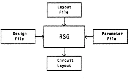
A circuit layout is generated from the following inputs (Figure 1.1): a design file, which is a parameterized, procedural description of the archi-tecture; a layout file, which is a graphical specification of cell layouts and interfaces; and a parameter file, which provides the size and functional

speci-9

(17)

Figure 1.1: RSG Layout Generation

fications for the particular case. By completely decoupling the graphical and procedural domains, a level of modularity is obtained which achieves local eficiency in layout generation, and global efficiency in the management of new architectures, layouts, and interfaces to other CAD tools.

The RSG also supports macro abstraction, i.e. the specification of macro-cells as interconnections of smaller macro-cells whose binding to actual layouts can be delayed to any desired time. In addition, interface inheritance relations provide a procedural means for defining interfaces between any two macro-cells: a new interface between two macrocells can he computed from any legal interface between a subcell in the first macrocell and a subcell in the second. As a result, macrocells can be used to specify even more complex cells in an entirely procedural manner with no need for additional layout.

At this stage of the discussion, all of the RSG's functionality appears to exist in other layout generators. For instance, procedural specification of circuit layouts is as old as silicon compilation itself, and essentially defines it. The novelty of the RSG is not its use of procedural specification, but rather

10

(18)

II·l-L---L-(I----the level of abstraction at which it is used. Failure to choose an optimal level of abstraction complicates the user interface, and forces the designer to concentrate as much on the internal constraints of the generator as on the functionality of the circuit being designed. Examples of this are layout generators that require placement of cells by strict abutment, or that do not support true hierarchical macro abstraction.

The significant contribution of the RSG is efficiency, not computability, of design. That is, the RSG does not produce any circuit layouts which, given unlimited effort, could not be produced by other layout generators. The result of this efficiency, however, is a tool that performs well in practice, not just in principle, in a realistic VLSI design setting.

1.2 Comparison with other layout generators

1.2.1 Module generators and Silicon Compilers

Specialized VLSI module generators produce layouts of a particular ar-chitecture to implement a specific logic function such as PLAs, ROMs, or Weinberger arrays. These module generators produce layouts of a specific style of implementation in a specific technology. For example a PLA gener-ator might generate PLA's with a standard NOR/NOR architecture, imple-mented with CMOS precharged gates. Such specialized module generators are capable of generating highly optimized layouts within the restricted class they are designed for. This is because these generators can incorporate spe-cific knowledge about the details of their particular implementation. For instance a PLA generator which incorporates knowledge about the

(19)

lar process technology and type of circuitry used can be made to size power busses and transistors according to some speed and power criteria. The dis-advantage of these specialized module generators is that their scope is limited to the applicability of the specific function they implement and to the specific process technology they use. Other module generators such as HPLA also generate a single architecture but allow freedom in the implementation and choice of technology. All of these module generators take as their input a configuration specification (in the case of a PLA this would be the number of inputs, outputs, product terms and the truth table) and not a high level functional specification, or an architecture specification because functionality of the output layout is implicit in the single architecture they implement.

Silicon compilers start with a functional specification as their input. How-ever current silicon compilers are not capable of determining and implement-ing the optimal architecture for a given functional specification and tech-nology. These programs use a single canonical architecture into which most functional specifications can be compiled to implement all functional specifi-cations. Their success depends on how well the canonical architecture they use is suited to the functional specification at hand. Macpitts[291 uses a data path implemented with registers, adders, and shifters, and a control path implemented with a Weinberger array as the canonical architecture. While such an architecture may be suited for some applications it clearly is not suited for applications in signal processing which require an efficient imple-mentation for multiplications. Hence even if the program succeeds in keeping the transistor density high by packing a lot of circuitry in a small area, the functional density measured by how much silicon it takes to implement a given functionality is low. This is due to the inappropriate implementation

12

__II--UIIUYI-. lil*··L·--UI---··II --1.-.---.-^1

(20)

Generality Efficiency

1 Canonical

Multiple

4 1 Architecture

Architecture

Architectures

per Function

1 Framework

* Macpitts

· RSG

* HPLA[6]

* Bristle blocks[14] * Multiplier Gen.[5]

· F.P. ALU Gen.[4]

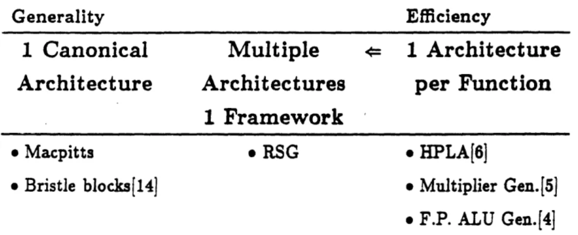
Figure 1.2: Comparison with other layout generators.

architecture where many more transistors are required than would be the case with a suitable architecture. Early versions of Macpitts required about 5 times the area than would be the case for layouts generated by hand.

Unlike specialized module generators and today's silicon compilers the RSG can generate many different architectures with just one framework. By matching the architecture to the functionality a level of generality greater than that of specialized generators can be achieved without the loss of effi-ciency incurred in current silicon compilers by a mismatched target architec-ture. Another big difference between silicon compilers and the RSG is that silicon compilers start with a function description of the problem whereas the RSG starts with user-defined primitive cells and cell connectivity information

(as shown in Figure 1.1). Figure 1.2 shows how the RSG is moving toward greater generality than specialized compilers without the loss of efficiency incurred in todays silicon compilers.

1.2.2 RSG as a superset of HPLA

The RSG expands the scope of HPLA by allowing many different archi-13

(21)

tectures to be generated with the same benefits as in the case of HPLA, but with just one framework. Though many of the features of the RSG can be explained and justified independently of HPLA, HPLA ideas have inspired and motivated the design of the RSG. HPLA does not support many of the key features of the RSG such as macro abstraction, inheritance and macro cell abstraction. Also the algorithms and software techniques used in the RSG are totally different from those used in HPLA. HPLA uses a cell reloca-tion scheme whereas the RSG uses interfaces and an interface table. However both the RSG and HPLA use the idea that adjacent (primitive) cells in the final layout interface in the same way as they do in the sample layout. Hence in both programs the (primitive) cell definitions and spacing parameters are extracted from a sample layout.

In HPLA the sample layout was an actual assembled PLA and hence had the same architecture as the final layout. This constraint that the sample layout be a fully assembled PLA is actually superfluous. Using the same methods as those used in HPLA (i.e. relocation) it is possible to achieve the same results from a sample layout consisting of the PLA cells with the only other constraint being that all possible interfaces that might occur in the final layout be present in the sample layout. The fact that the sample layout was a two input, two output, two product term PLA was simply a way to ensure that all the required cells and interfaces between them be present in the sample layout because the architectural specification for PLAs is already hard coded in the HPLA program itself and is not extracted from the sample layout.

In the RSG this constraint is relaxed. This not only reduces the size and complexity of the sample layout, but it also allows the same sample layout

14

(22)

to be used in output layouts of various different architectures because the implicit architecture always present in the sample layout does not constrain the architecture of the final layout. The sample layout in HPLA was actually larger than necessary and contained redundant information. For example the sample layout for HPLA contained 2 (identical) instances of the and-sq connect-ao interface when only one was required. In so doing it increased the number of instances of and-sq and connect-ao making the sample layout larger than necessary. The cells in many PLA sample layouts can also be used to generate other layouts besides PLAs such as decoders and multiplexors (decoders can be built from an AND plane with appropriate output buffers). Hence requiring that the sample layout look like the finished product is not only an unnecessary restriction it also reduces the scope within which any given sample layout may be used.

The method (relocation) HPLA uses to generate new cells does not eas-ily lend itself to cell hierarchy. This did not matter in HPLA because the architecture that HPLA generates (i.e. the architecture for standard PLAs) does not make use of cell hierarchy. Making use of cell hierarchy entails gen-erating a macro cell from the primitive cells in the sample layout replicated according to some parameter, and then calling the new macro cell in an even higher order cell several times according to some other parameter. In the relocation scheme the cell definitions for subcells of a higher order cell are actually modified to suit the needs of the calling cell. This worked fine in HPLA because there was only one calling cell, i.e. the complete layout of the PLA. In a scheme which uses hierarchy there may be many higher order cells (which can possibly be called in even higher order cells), that call the same subcell. Each of these cells may request that the called subcell be modified in

15

(23)

some particular fashion to suit its specific needs. These modification requests can be conflicting. One way to solve the problem would be to create a copy of the subcell for each of the calling cells. Hence each calling cell can modify its copy of the subcell without conflicting with the modifications requested by the other calling cells. The RSG however uses a simpler and more powerful technique where this problem does not occur.

1.2.3 The description file verses the interface table.

Before HPLA can make a PLA from a sample layout it must first compile the sample into a special file called the description file. This description file contains the definition of all the. key cells where the cell definitions have been modified as prescribed by the relocation scheme. It also contains the spacing parameters (pitches) for the various cells. In HPLA, for the users convenience, the process of making a PLA is divided into three parts each of which occur at different times in the design cycle. This division of the generation process allows delayed binding of the specifics of the PLA encoding until after the PLA is fully installed into the rest of a layout. The description file is accessed at each of these three phases, hence it makes sense to create the description file just once and refer to it in each of the three phases of the PLA design.

In the case of the RSG the data structure corresponding to the description file would be the interface table. However since the RSG produces the whole layout all at once, it does not make sense to store the data structure into a file and load it back immediately into the workspace and use it during just one session. Therefore no temporary file is created.

The RSG can generate any PLA that HPLA can. It can also generate 16

(24)

more complex PLAs such as PLAs with folded rows or columns. However in HPLA the division of the generation process into three parts facilitates recoding the PLA (or postponing its encoding) and speeds up the plotting of the chip by leaving out the PLA's crosspoints until required, making HPLA a little more convenient to use.

1.3 Thesis organization

* Chapter 2 lays down the mathematical foundations of interfaces, the method the RSG uses for local placement constraints.

* Chapter 3 gives the overall RSG algorithm .

* Chapter 4 Describes the Language for specifying design files and de-scribes in more detail the specifics of the underlying data structures. * Chapter 5 Describes the design of a class of pipelined multipliers using

the RSG.

* Chapter 6 Is concerned with issues relating to building a special type of compactor for use with the RSG.

Each chapter is organized so that the first Sections lay down the concept and the foundations of the method and the last sections go into the details of some important facet of the problem.

17

(25)

Chapter 2 Interfaces

2.1 Cells and Instances

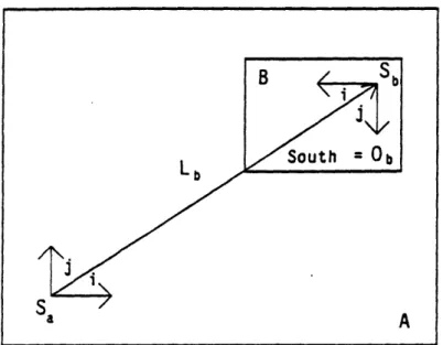
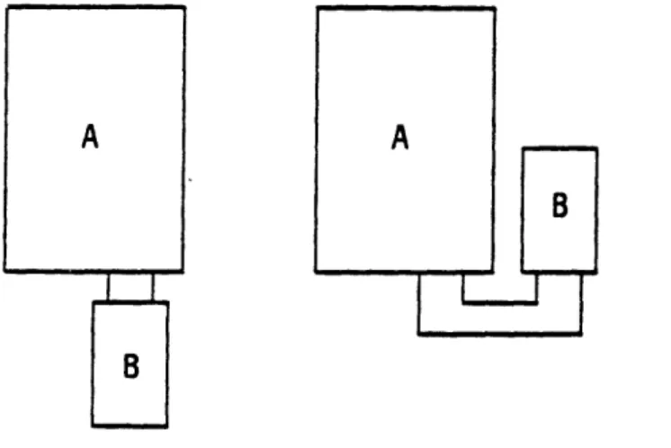
The RSG requires user-defined cells to hierarchically build larger cells. A cell A consists of objects whose locations in the cell axe defined in terms of a local coordinate system Ca with origin S,. The objects in A can be boxes of various layers, points, and instances of other cells. An instance of a cell B is the triplet (L, O, (cell definition)) where L is the point of call of the cell B, 0b is the orientation in the call of B and (cell definition) is a pointer to the cell definition of B (the superscript ' means that the location or orientation is relative to a calling coordinate system). The effect of having an instance of B in A with point of call L and orientation O' is that of performing the isometry' O' on B ( is an isometry that leaves Sb, the origin of the coordinate system within B unchanged), placing the origin Sb of B at location L within the coordinate system of A, and finally adding to 'An isometry is either a rotation or a reflection.

18

(26)

Lb

Figure 2.1: Instance of cell B in cell A. A the collection of objects in B (see Figure 2.1).

2.2 Interface Definition

A key notion in the RSG is the interface. If instances of cells A and B (the cells A and B do not necessarily have to be distinct) are to be called within the same coordinate system, then cells A and B have an interface between them. The interface between two cells A and B is the ordered pair

Ia = (Va,

oab)

(Ib 0 Iba) where Vb is the interface vector and Ojb is the interface orientation. Vab is the vector whose starting point is the point of

call of A and whose endpoint is the point of call of B, if the instance of A is held at orientation north (identity transform). Oab is the orientation that B would have if the instance of A were held at orientation north.

Treating the orientations as operators with uo" being the operator com-19

A

-_ _ ___ _

(27)

position rule we have2:

o,,b

= (O:)-' o (2.1)

Vb = (a)-' (L- L) (2.2)

The interface vector Va and interface orientation Oa are obtained by deskewing the relative orientation of B i.e. and the vector (Lb - La) by the inverse orientation of A (O)'- .

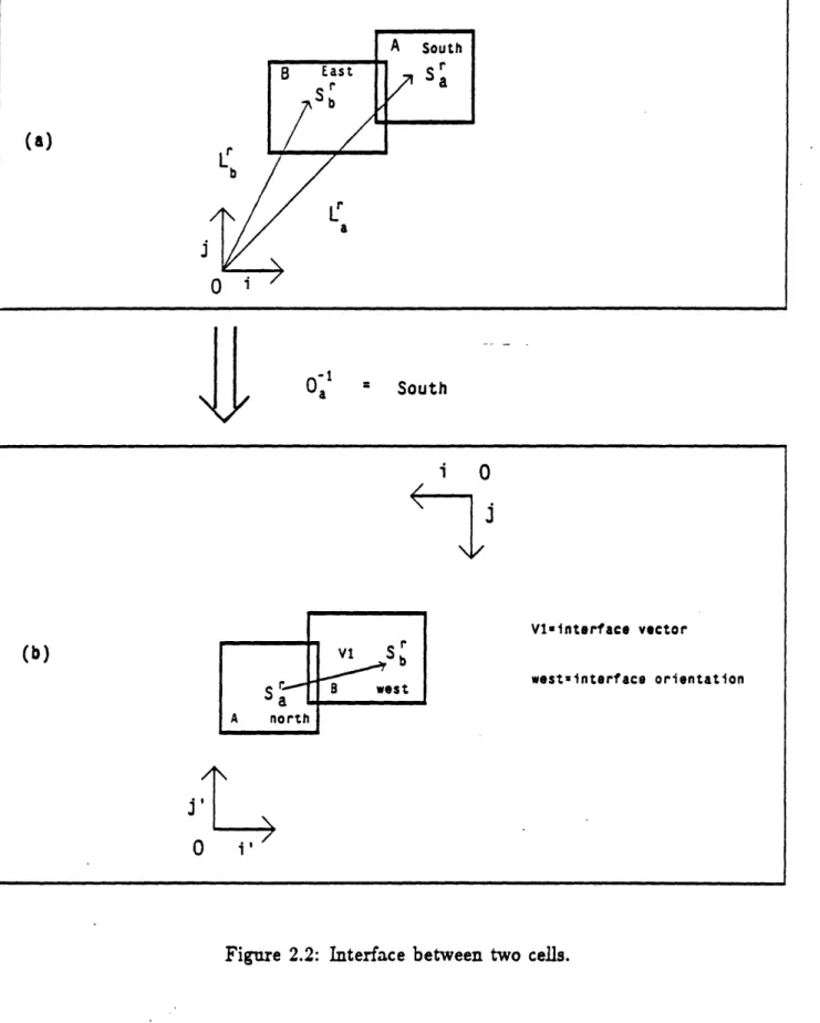
Figure 2.2(a) shows an instance of A and an instance of B called together in a same higher order cell (characterized in the Figure 2.2(a) by it's coordi-nate system (O, i, j)). The point of call La (respectively L) of A (respectively B) is the location where the origin of A (respectively B) is placed in the call-ing coordinate system (O, i, j). In order to obtain the interface Iab between A and B we must first perform an isometry on the calling cell (the one with the (O,i,

j)

coordinate system in Figure 2.2(b)) such that the new orientation for the instance of A will be North. Since A is initially oriented South the calling cell must be reoriented by South-

'

= South (because 180° = -180° ) so that A will ultimately be oriented North. Figure 2.2(b) shows the result of the transformation of the calling cell. The interface vector is now the vec-tor whose starting point is at the new point of call A and whose endpoint is at the new point of call of B. The coordinates of the interface vector are computed in terms of the new basis (i', j') which is the same as the old basis (i,j) of the calling cell before the transformation was performed. The inter-face orientation is now the the new orientation of B after the transformation was performed.

The existence of an Iab interface between A and B automatically gives

20 - l is defined by O-l o O = o 0-1 = Identity.

20

(28)

O- = South

i 0

Vl-tnterface vector

westrinterface orientation

o

i'

Figure 2.2: Interface between two cells.

21 (a)

j

Ea a (b) __

(29)

rise to an interface In between B and A. The expression for the Ib, interface can be obtained from equations 2.1 and 2.2.

Oba ₌ _{O, o Ob} = ( 100b)-o 1 = 0b (2.3) (2.4) ba = O (La-L) = (O' o (O o O'))-(L - Lb) = ((b o O,) o ;0,1_{)(La - Lb)} = (Oa o o')(La - Lb) - (0 ' o 0,')(L, - Lb) = -062(0; (L₆ - L,)) - aVob

Therefore Ia = (Vb, Ob) =(-O va, o).

2.3 Advantages of using interfaces

Interfaces are a natural way of defining the relative placement and orien-tation between instances of cells. Hence knowing the calling information of a cell A in a cell C and knowing the interface between A and B it is pos-sible to determine the calling information of B in C. The RSG allows the user to specify the primitive cells and interfaces between them graphically, by providing a layout file which will henceforth be referred to as the sample

layout. The sample layout contains the definitions of all primitive cells as well as interfaces between them. An interface between cells A and B can be defined by calling A and B together in a higher order cell C with the

appro-22

(30)

priate relative placement and orientation between them. In practice when new cells are created by the layout designer they are assembled together in order to verify that the different new cells that have been designed, do in fact interface properly to each other. The simple fact of assembling the cells together requires calling them both in one cell (same coordinate system) and therefore automatically defines an interface between them. Hence interfaces can be designed at almost no extra cost to the designer.

By virtue of the design-by-example feature of the RSG, the relative place-ment of neighboring cells in the final layout is such that each interface in the final layout is an instance of an interface in the sample layout.

Since the relative placement of cells in the final layout is performed using interfaces between cells and not by using the sizes and shapes of the bounding boxes of those cells, the cells can be designecd according to their functional boundary constraints and without regard to abutment constraints. Not only does this make cells easier to design and design rule check (because instances of cells can overlap, each cell can be made design rule correct3), the fact that cells are not cut at artificial boundaries helps reduce the proliferation of cells of essentially the same functionality but different abutment constraints. Us-ing interfaces also allows cells to be easily encoded by superimposUs-ing several cells in order to modify the functionality of a basic cell. This too helps in reducing the proliferation of different cell types since the number of different encoding configurations is roughly exponential in the number of independent encoding decisions.

Cell encoding can also simplify the personalization process since instead of combining all the encoding decisions together to select a single cell of the

3_{Some hierarchical design rule checkers require that instances do not overlap.}

(31)

appropriate type we can use each independent encoding decision to perform a simple encoding masking of one basic cell. An encoding cell may lie well within the bounding box of the cell it encodes and hence placement by abut-ment would be cumbersome since it would cause a proliferation of (spacing) cells that have nothing to do with functionality. By simply specifying an interface the relative orientation of the cells as well as whether the cells are side by side, one on top of the other, or one inside the other, is handled automatically.

2.4 The Interface Table

The RSG program maintains an interface table of all legal (user specified) interfaces between cells. This table is first initialized with interfaces from the sample layout and can be augmented as new cells are created by the system. Since there can be several different legal interfaces between two cells there can be a family of legal interfaces between two cells A and B. Figure 2.3 shows two different possible interfaces for a pair of cells A, B.

If the set of legal interfaces between any two cells is indexed over the integers then the interface table can be described as a mapping from triplets: ((cellnamel), (cellname2), (interface index number)) (2.5)

to interfaces:

((interface vector), (interface orientation)) (2.6)

If Ib is an interface in the interface table, then Ib, the corresponding interface between B and A, is also loaded in the interface table. Hence knowing the

24

(32)

VI _ west A north Vitinterface vector westainterface orientation V2zinterface vector south-interface orientation Interface#2

Figure 2.3: Different Interfaces between two cells.

placement of A one can determine the placement of B and vice versa. This bilaterality of the interface table is very important. We will see in section 3.4 that it may not be possible to determine in advance which of the two instances A or B has a known placement and which one will have its placement derived from the other.

2.5 Interface Inheritance Relations

In order for any cell to be used in the RSG it must have an interface with some other cell, otherwise there is no way to place it. When new cells are built up hierarchically by the system, in order to take full advantage of cell hierarchy, interfaces for new cells can be specified in terms of existing ones. In this way cells built up by the system can be used to build even larger cells

25

Interface#1

(33)

Icd new

Iab

existing

Figure 2.4: Interface Inheritance

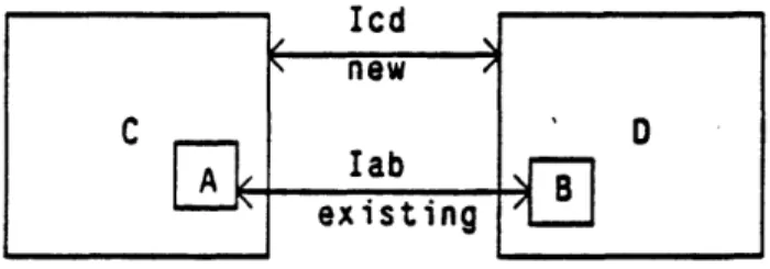
in exactly the same fashion as were the primitive cells of the sample layout. If A (respectively B) is a subcell of a new cell C (respectively D), it is then possible to define a new interface Id between C and D in terms of an existing interface Iab between A and B. Id is the interface that C and D would inherit if the subcells A and B within C and D were placed and oriented with interface Ib (see Figure 2.4). The RSG allows the user to define a new interface (and load it into the interface table) by specifying the two cells C and D, the instances of A and B in C and D, the interface

number of the interface between A and B and an interface number for the newly defined interface between C and D.

The rest of this section is concerned with finding an algebraic expression for the interface vector and interface orientation of the new interface Id between C and D in terms of the existing interface In between A and B and the calling parameters of the instances of A and B in C and D. Let' (L, Ore),

(respectively (Lrd, Od)) the calling information of A (respectively B) in C (respectively D) and (Vb,-Oab) (respectively (Vcd, Ocd)) be the interface vector

4The superscripts "c (respectively ?d) mean that the locations and orientations are relative to the coordinate system of C (respectively D).

26 C Wi ' O

-E

111-.. --^ 1111----··----·-··"T·rr .--...* - .

(34)

-and interface orientation of Iab (respectively Icd). Also let L; (respectively LL,LL) be the location of the origin of A (respectively B,C,D) in the implicit calling coordinate system (i.e. as they appear in Figure 2.4) and let O (respectively O, O, 0 ) be the orientation of A (respectively B, C, D) in the implicit calling coordinate system (which can be for argument sake considered to be the absolute coordinate system) then:

o = o o (2.7)

L = L; + O;Le (2.8)

and

= f o 0od (2.9)

L; = Ld + O;Ld (2.10)

Replacing 2.7 and 2.9 in 2.1 we get:

0o = (O')- oO°

= (o 0

o

0 C)1 o o o Ord

= (O)- I o (;) - o o = o d d ) ^ = (Or)10(Or)-1o0r

O°c o 0 o ab (Ord)-1 = (or)-1 oo = Ocd

So

Ocd = o oab o (O 1 (2.11)

Replacing equations 2.8 and 2.10 in equation 2.2 we get: 27

(35)

Vob = (O )-1(L- L)

= (Or)-'(L' + OLb - OrLr)

L

-

L

= OrV

-

OLrb +

OLCr

(O )-1(L - L- ) = ((O-)-l O)Vab ((O)-l O)L;b + (O)-' o (OL C)

Using equations 2.2 and 2.1 with different subscripts, equation 2.7 and the previous result we get:

vcd = (O)-'(L-Ld)

= ((c) ° Oa-)Vb - ((°o)- °o,; )Lb + ((o)- o O)Lc (2.12)

OcVab - (Or)-'L b + Lre

2.6 An efficient representation for orientations

Whereas interface vectors can be straightforwardly represented by a pair of real numbers, orientations require a slightly more complex data structure. The purpose of this section is to find an efficient representation for orien-tations in terms of memory, computation and ease of manipulation. Recall from Section 2.1 that calling an instance of B in A consists of performing an affine isometry to the objects in B and then adding the collection of objects in B to A. A layout editor needs to be able to perform affine isometries on the various cells. If A is called in a cell B which is in turn called in a higher order cell C then two affine isometries get applied to the objects in A. The first isometry I corresponds to the calling parameters of A in B and the second isometry I2 corresponds to the calling parameters of B in C. For an object Ob in A the corresponding component in C would be I2(I,(Ob)). I is

first performed on Ob and then I2 is performed on the resulting object. Another way to perform isometry composition is to first compose the two operators and then apply the resulting operator to the object. Since

28

(36)

--I2(,(Ob)) = (I2 o I)(Ob) it is possible to first compute (I2 o I) and then

apply this new transformation to Ob. This method of first computing the resulting isometry and then applying it to the object can be computationally more efficient as the resulting isometry is computed only once and hence effort is not duplicated over the various objects on which this transformation is to be performed.

In layout editors the preferred way of composing operators could be I2(11

(Ob))

because this method is easier to implement 5. If there is already a method for performing isometry on objects then, since the result of applying an isometry to an object is an object of the same type no extra mechanism is needed to successively perform several isometries on the object. In the case where only a finite set of legal isometries are implemented this method can lead to more efficient methods for applying single isometries to objects. For example one could index the set of available isometries over the integers. In that case, in order to apply a isometry known by its index number to a given object, one could use the index number to lookup a table of procedures (there is one procedure per isometry) to get the procedure that implements that particular isometry and then apply it to the objects. This method elim-inates the interpretive overhead associated with the decoding of the isometry representation. For example isometries can be represented as matrices, and a program that can apply any matrix transform to an object would be slower than one that performs an unique fixed linear operation. However this in-dexed representation does not lend itself to symbolic composition. If the number of implemented indexes is n then (assuming that the set of

imple-SHowever HPEDIT uses the 12 o I method. 'HPEDIT uses this method.

29

(37)

mented isometries is closed under isometry composition rules) knowing the index of I2 and the index of I in order to compute the index of (I2 o I,) a

mapping table from n * n to n integers is required. Another table from n to n integers is also required to invert the isometries (assuming the set is closed under inversion). Hence this method becomes cumbersome in the case where there is a large number of implemented isometries. It also requires a large number of procedures; one for each implemented isometry.

In the RSG at times it is necessary to obtain expressions for new trans-formations and therefore operations for symbolic composition and inversion of transformations are required. Recall equations 2.11 and 2.12 from Sec-tion 2.5. In order to compute the new inherited interface vector and interface orientation, we need to obtain expressions for the composition and inversion of orientations. It is therefore necessary to have a representation for orienta-tions that allows them to be easily applied as operators and also allows them to be easily composed and inverted.

One possible way to implement all orientations is to use 2 * 2 matrices of real numbers. 2 * 2 matrices of real numbers can however represent all the different linear transformations in the vectorial plane out of which isometries

(which are orientations) are only a very small subset. As a result they require storage and manipulation of much more information than is needed. Matrix composition and inversions are also relatively costly computationally.

There are more compact representations for orientations. We can rep-resent all the vectorial rotations in the plane with a real number between [0, 27r[. The rotation can be expressed by the complex number e'i where j belongs to 0, 27r[ and i2 = -1. Orientations are either rotations about the origin or reflections about an axis passing through the. origin. All the

reflec-30

(38)

-tions about an axis passing though the origin can, however, be generated by composing the reflection about the y axis (or any other axis passing though the origin) with a rotation about the origin. If M is the interval [0, 27r[ and B is the set of Booleans, it is then possible to represent an orientationby the pair (j, k) E M * B where j represents the rotation, and k indicates whether or not a rotation about the y axis is to be performed before the rotation (the composition of rotations and reflections is not commutative). If + (respec-tively -) is the induced addition (respec(respec-tively subtraction) modulo 2r from M to M and if R is the rotation about the y axis. Than any orientation can be written as: ei o R where (j, k) i M * B and i2 = -1.

2.6.1 Inverting two orientations.

Let 0 = ei o Rk and 0 -1 = e'i o Rk'

* If k = 1, then 0 is a reflection. Therefore 0 o 0 = I where I is the Identity transform and hence

0-1 =0

= ii o M (2.13)

i_{' o M}

so j = j' and k = k

* If k = 0, then O is a rotation and hence 0 - 1 = eij'

- 1 (2.14)

so j' = -j and k = k'

(39)

Hence If k = 1 then j = j', k' = k otherwise j = -j', k' = k

2.6.2 Composing two orientations

Let

0 =

i j

oR

i ' 02 = 42

OR

k (2.15) 0 = 02001 = eisoRk Then O = (ei0i o R*k ) o ei

Rk)

(2.16)

= eiJ2 o (R o ei j_l) _{o Rk}

because of the associativity of linear operators. * If k2 = 1 then

R"2 o e'iJ is a reflection and hence (R" o ci' j' ) _{o (R" o}

_eijl)

_{= I}

_therefore

Rk

o eiil =

(R"

o

eiul)-L

= (eiil)" o (R,)-1

(2.17)

=

ei(-l)

o R

(i(-il))

o

(Rk,)

because Rk2 is a reflection (or identity) and ei'l is a rotation. therefore O = eij' o (Rk2 o eil)oR kl = C , o (i(-) o

(R,))

o

Rk, = (ei2 o0

e(-il))

o (R2 o R"') (2.18) = (~ei( ,1) ) o (R*k2l) = ei(-J,) o

(R k)

32

(40)

--where iE is the XOR operator. hence j = j2 - Jl and k =k *If k2 = 0 then 0 = eii2 o (Rk2 o eiil) o Rk = eit3 o (Cit7)

o

Rk (2.19) = (eij2 oe i _{) o Rk}t - ei(j l + )o R hence j = j2 + Al and k = k

So Hence If k2 = 1 then j = 2 - il., k = kl otherwise j = ji + .2, k = kl

We have seen that we can represent an arbitrary orientation (isometry) by the pair (j, k) E M * B and.using the associativity of linear operators we can compute any expression involving composition and inversion of orientations. It is computationally expensive however to apply an operator represented in this form to actual objects, because a sin an a cos must be computed. Due to numerical inaccuracies an object (say a box) with vertical and horizontal edges can be transformed by a quarter turn rotation into a object whose edges are not precisely aligned with the axis. Adding and subtracting elements of M can also lead to numerical inaccuracy as elements of M are represented in the computer by real numbers and a modulo 27r operation has to be performed on the result of every real addition (or subtraction) to ensure that the result is an element of M.

In the RSG the choice therefore was made not to support arbitrary ro-tations and reflections. Most VLSI circuit layouts are built using boxes of various layers where the boundaries of the boxes are vertical or horizontal lines i.e. parallel to one of the coordinate axis. Hence in most cases it is

33

(41)

sufficient to support all orientations that transform vertical and horizontal lines into vertical and horizontal lines.

The four multiples of the quarter turn rotation are the only rotations that have this property. The only reflections that can have this property are those that transform vertical edges into vertical edges and horizontal edges into horizontal edges which are the two reflections about the axis. And reflections that transform vertical edges into horizontal edges and vice versa which are the reflections about 45 degree lines passing through the origin. These 4 reflections can be generated by first reflecting about the y axis and then applying one of the four quarter turn rotations.7

Just as arbitrary orientations can be represented by an element of M * B, these eight basic orientations can be represented by z, an element of

(4 = {

1,

2,3}), and a boolean

k,

hence by an element of *

B.

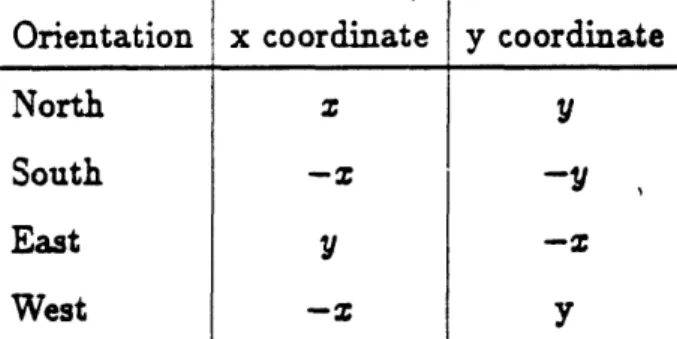
This

would correspond to the orientation e i' o R in the previous notation. Using the induced addition and subtraction on the rules for composing and inverting orientations are the same as previously described using the M * B representation. Orientations can now easily be applied to vectors and boxes since performing a reflection about the y axis corresponds to changing the coordinate of an object to -. The four quarter turn rotations require only permutations and negations of the two coordinates. For instance the one quarter turn rotation maps the x coordinate into the y coordinate and the y coordinate into the -z coordinate. The Figure 2.5 shows the mapping of coordinates for each of the four basic rotations.

?these are the 8 orientations also supported by HPEDIT.

34

(42)

Orientation Ix coordinate y coordinate

North z

South -z -y ,

East Y -z

West -z y

Figure 2.5: Coordinate mapping for the 4 basic rotations

35

(43)

Chapter 3 The Algorithm

3.1 Algorithm Overview

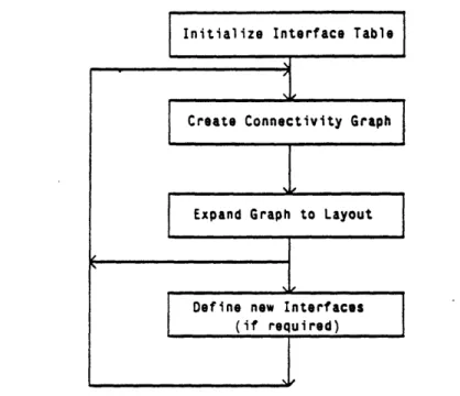
The RSG algorithm (see Figure 3.1) consists of first reading in the sample layout in order to define the primitive cells and build up the initial interface table.

New cells are then created in a two step sub-algorithm. The first step in the sub-algorithm consists of building a connectivity graph for the new cell. The connectivity graph for the new cell is a graph whose vertices represent partial instances whose cell type is known but whose location and orientation are as yet unspecified.

The edges between vertices represent interfaces between instances and the weights assigned to them are the interface index numbers. The connectivity graph need only be a spanning tree since cycles in the graph contain redundant information. For a given sample layout, each connectivity graph gives rise to a unique layout (see Figure 3.2). Interfaces provide the local placement constraints between (two) cells. The connectivity graph provides information

36

(44)

Initialize Interface Table

Create Connectivity Graph

Expand Graph to Layout

Define new Interfaces uired)

Figure 3.1: RSG algorithm

about the global placement of all the subcells in a macrocell. The graph sets up an implicit system of linear equations whose unknowns are the placements and orientations of the (pseudo) instances in the graph and where the given parameters are the interfaces between the various cells.

Interfacel#

1

(if req

Figure 3.2: Graph and Layout Equivalents 37 rI .ii [i, i i~~~~~~~~~~ ! . [ iii ii -l ii i ] · ,_ __ I

(45)

The second step consists of converting the connectivity graph into a layout. This is done by first selecting a root node in the graph and arbitrarily placing and orienting the corresponding instance. The graph is then traversed, and each of the nodes in the graph (which initially are all partial instances) gets expanded into a complete instance with a location and an orientation. The location and orientation Lb and Ob of a partial instance B can be computed from the location and orientation La and 0. of one of its already traversed neighboring nodes A using the formula,

Ob = Oa 0 ab (3.1)

Lb =

OVhV

+ La (3.2)

where (Va, Oa0) is the interface between A and B. Finally once a new cell is created, if it is to be used in a larger cell, it is necessary to define new interfaces between it and the already existing cells.

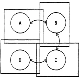
Since the connectivity graph need only be a spanning tree many of the interfaces that occur in the final layout need not be present in the sample layout. Figure 3.3 shows a cluster of instances of A, B, C and D assembled together. The corresponding connectivity graph is also shown. The labels inside the nodes of the connectivity graph correspond to the nodes a well as the instances they are contained in. Since the connectivity graph need only be a spanning tree, it does not have to contain edges between A and D, A and C, or B and D. This is because with or without those edges the graph remains a single connected component (i.e. one can reach any node starting from any node by walking along edges in the graph). Since the three described edges are not present in the graph the I (or Id4), I, (or I,.), and I (or Idb) are never accessed by the RSG, and therefore need not

38

(46)

Figure 3.3: Graph Connectivity Requirements

be present in the sample layout. Hence the creation of both design file and sample file is simplified by requiring that the graph be only a spanning tree.

3.2 Advantages of the method

This (augmented) two step process of first determining connectivity and then using the connectivity information along with cell definition and cell interface information to build a layout, provides a clean separation between the graphical and procedural information. The procedural information in the design file is used to build the connectivity graph and remains constant over different implementations of the design as given by the sample layout.

The graphical information from the sample layout is used to transform the connectivity graph into a physical layout of a particular implementation of the design. Cell spacing parameters which relate to the graphical information are never accessed or manipulated in the design file. This delayed binding on the

39

(47)

location and orientation of instances allows for clean macro abstraction in the design file. Since in the design file, partial instances are connected together without assigning actual locations and orientations to them, it is possible to build subgraphs without prior knowledge of where and with which orientation the instances in the subgraph will be used. It is easier and cleaner to write and compose macros for sub-graphs, because the state of a calling macro does not side-effect the called macro by imposing a starting location and a starting orientation at which to start assembling the subcells (i.e. the called macro returns the same subgraph regardless of how the calling macro will choose to connect the subgraph and regardless of the final calling parameters of the instances of the subgraph). Macro abstraction suppresses details of how and where a macro for generating a subgraph gets called and allows the designer to concentrate only on the connectivity of the subgraph.

3.3 Limitations

The two step process as described in the previous section provides a high level of separation between the graphical and procedural part of the layout process. Since geometrical parameters are not accessed in the design file, however, decisions based on the size and shape of the final layout such as placement and routing are difficult to make. For example the choice between the two routing configurations in Figure 3.4 requires knowledge of the sizes and shapes of the two cells A and B as well as the size of the routing channels.

40

(48)

--Figure 3.4: Different routing configurations

3.4 Connectivity Graphs in Greater Detail

The purpose of this section is to investigate some of the properties of connectivity graphs both in terms of data structures as well as in terms of their mathematical properties. The previous section described an equivalence between connectivity graphs and physical layouts. Actually (for a given sam-ple layout) to each connectivity graph there corresponds a whole equivalence class of layouts. All the layouts in an equivalence class are such that any ele-ment in the class can be transformed into any other eleele-ment in the class by an affine isometry i.e. all elements in an equivalence class are identical modulo an affine isometry. By selecting a root node in the graph and by placing and orienting the corresponding instance a particular element in the equivalence class is identified, namely the one where the instance corresponding to the root node has the chosen placement and orientation.

Connectivity graph data structures must have bilateral edges. If there is an edge between nodes A and B then in the data structure of A there must be a pointer to the data structure of B and in the data structure of B there must be a pointer to the data structure of A. This is because when a connectivity

41

(49)

graph is being created, the root node of the graph (which is arbitrarily chosen,

placed and oriented) which is the starting point for traversing the graph (in

order to convert the graph into a layout) may not be known. Macros for

generating subgraphs of a layout have no knowledge of how the subgraphs

they generate will be connected together by their calling macros in order to

make larger graphs. For example if a macro M for creating graphs were to

return the subgraph of Figure 3.2, either node B or node A could be a leaf

node in the graph (i.e. a node with only one connection to it) depending on

whether node A or node B was connected to the rest of the connectivity graph

by the macro that called M. Hence even if the graph is a spanning tree the

parent-son relationship between directly connected nodes in the graph is not

known until the graph is traversed. This is why during the graph traversal

one must be able to get to node B from node A and also get to node A from

node B because we do not know which of the two nodes will be visited first.

The bidirectionality of the graph is essentially a data structure problem

that is constrained only by the graph traversal requirements and not by the

abstract mathematical properties of the graph. This requirement does not

constrain whether or not the graph is directed or not. A graph G = (N,E)

where N is a nonempty set of nodes and E is the set of edges is said to be

directed if the edges are ordered pairs (v,

to)

where (v, to) E N * N. That is

to say there is a privileged direction for the edges of the graph. A graph

G = ({A,B},(A,B)) (a graph with nodes A and B and an edge from A to

B) can have a bilateral data structure which means that from node A we can

go to node B and vice versa, and can at the same time be directed which

means that the (A, B) edge has a privileged direction (i.e. the (B,A) edge

may not exist).

42

(50)

Interface#1

/7

-Interface#1

Figure 3.5: Interface ambiguity in undirected graphs.

We now need to decide whether or not connectivity graphs for the RSG should be directed graphs or non-directed graphs. What is needed is a graph that for a given sample layout uniquely defines an output layout (modulo an affine isometry). If the celltypes of nodes A and B are distinct then knowing the locations and orientations of node A it is always possible to determine the placement and orientation of node B because the right hand side of equations 2.1 and 2.2 are well defined. Hence at first it would seem that an undirected graph would suffice. However, in the case of Figure 3.5, if we know the location and orientation of the left node, there are two possibilities for the placement and orientation of the right node.

If In = (Vob, Oab) is an interface between A and B then using equations 2.1 and 2.2

43

dl

-/ 10_

(51)

Ib. = (V.,Ob.)

= (I ,)- _l _(3.3)

= (-(Oa)-V, (o)-l) is an interface between B and A.

Therefore if Io, = (V,, O,.) is an interface between A and A then

r. = (V.,O)

= (I)-1 (3.4)

=(-(O ) V,. (0)-1)

is also an interface between A and A. In equation 2.1 and 2.2 it is not clear whether V, and 0, or V' and O' should appear on the right hand side of those equations. The problem here is not that of determining the right interface index (interface number) so as to choose the right interface from the interface table. The real problem is determining which instance the left node in Figure 3.5 refers to. Another problem which we will deal with later is that we do not know which of the two interfaces I, or

r'

gets loaded into the interface table. The two interpretations of Figure 3.5 can lead to non equivalent layouts as shown in Figure 3.6. If the edges are undirected then there is no way to discriminate between these two cases. In the first versions of the RSG this problem caused the final layout to depend on how the graph was actually traversed. What is needed is a way of discriminating between the two nodes of Figure 3.5 which are directly connected together and have the same celltype. This can be done by giving privileged directions to the edges in the graph (making the graph a directed graph).

If we are able to characterize interfaces according to some criteria so as to discriminate between the two possible interfaces I, and I' and select one

44

(52)

I-Interface#l

Figure 3.6: Layout ambiguity for undirected Graphs.

45

1

B A

/ \/

1 A C

d

fcS

,ce#1 _ __ _ I __

(53)

L.:-T?& D M4-LnIILUI 4f.ac

Figure 3.7: Resolving layout ambiguity with a directed graph.

of them (which I will refer to as IO,) then with the convention that if there is a directed edge in Figure 3.7 from Al to A2 (Al and A2 have the same

celltype: the indices are just to distinguish between the two of them) then it is A1 that serves as the reference instance i.e. Al refers to the instance in

the interface (see Figure 3.7) that is deskewed to orientation North and at whose point of call the interface vector begins. Knowing the placement and orientation of A1 we can determine the placement and orientation of A2 using

equations 2.1 and 2.2 where the interface

I,

and knowing the placement and orientation of A2 we can determine the placement and orientation of Al

using the interface (Io)-'. The main problem has been to determine when to use (I°.) and when to use (I.,) - ' and this problem has been solved by making the edges of the graph directed.

The problem that now remains to be solved is that of selecting I1, from I, and I. One possible way to perform the selection process is to math-ematically characterize a property that is possessed by only one of the two interfaces I or I'. This property cannot depend on the interface

vec-46

K >.

II_IYLI___W_I1IIIlllllll____·iC1 li--·----L IIII1I 1

(54)

tors alone because it is possible to have I,a I with Va, = V' making the selection between I, and I'a using V, and V' impossible. Foe exam-ple if

I,,

= (O,East) then I = (I,)'1 = (, West) hence V, = V' and I,, # I. Similarly the property cannot depend on the interface orientation alone because it is possible to have I,. :

i,

with O,, = O' . As an example Let I = (V,, North). Then I = (-V,,,North). Hence O,, = O' and Iaa I,,

Since any reasonable mathematical criterion for selecting between I a and

I depends on both the interface vector and the interface orientation, chances for finding a simple user understandable selection criteria are seriously jeop-ardized. The user does in fact need to know which of the two interfaces gets loaded into the interface table , because the effect of loading (I0,)-' in the table instead of I°a is that of inverting the direction of all the edges (with the appropriate interface number) between nodes of celltype A.

The RSG solves this problem by allowing the user to specify (in the sam-ple file) the right interface by graphically discriminating between the two instances of Figure 3.7 (which might occur in the sample file). If it is pos-sible to graphically identify Al in the sample file then it is pospos-sible to force

I0 = (V o,

O0)

(see Figure 3.7) to be the interface that gets loaded into the interface table by forcing Al to be the reference instance at whose point of call the interface vector begins and whose orientation is deskewed to North.

We have seen that the connectivity graph data structure must have bilat-eral edges but that the graph itself must be directed. Only the edges between nodes of the same celltype need to be directed as direction information on

edges between nodes of different celltype is not used.

A design by example Regular Structure Generator

A Design by Example

Regular Structure Generator

Technical Report 507

A Design by Example

Regular Structure Generator

Technical Report 507

Abstract

Acknowledgments

2

Contents

List of Figures

Chapter 1

Introduction

1.1

Motivation

1.2

Comparison with other layout generators

1.2.1

Module generators and Silicon Compilers

1 Canonical

Multiple

4

1 Architecture

Architecture

Architectures

per Function

1 Framework

* Macpitts

· RSG

* HPLA[6]

· F.P. ALU Gen.[4]

1.2.2

RSG as a superset of HPLA

1.2.3

The description file verses the interface table.

1.3

Thesis organization

Chapter 2

Interfaces

2.1

Cells and Instances

2.2

Interface Definition

oab)

o,,b

j)

'

o

i'

j

2.3

Advantages of using interfaces

2.4

The Interface Table

2.5

Interface Inheritance Relations

-E

o

L

L

= OrV

OLrb +

OLCr

2.6

An efficient representation for orientations

(Ob))

2.6.1

Inverting two orientations.

2.6.2

Composing two orientations

Let

0 =

oR

OR

Rk)

(2.16)

eijl)

therefore

Rk

_eijl)

_therefore