Calibration and assessment of electrochemical air quality
sensors by co-location with regulatory-grade instruments
The MIT Faculty has made this article openly available.
Please share
how this access benefits you. Your story matters.
Citation
Hagan, David H. et al.“Calibration and Assessment of
Electrochemical Air Quality Sensors by Co-Location with
Regulatory-Grade Instruments.” Atmospheric Measurement
Techniques 11, 1 (January 2018): 315–328 © 2018 Author(s)
As Published
http://dx.doi.org/10.5194/amt-11-315-2018
Publisher
Copernicus GmbH
Version
Final published version
Citable link
http://hdl.handle.net/1721.1/114971
Terms of Use
Creative Commons Attribution 4.0 International License
1Department of Civil and Environmental Engineering, Massachusetts Institute of Technology, Cambridge, MA 02139, USA 2Department of Civil and Environmental Engineering, Virginia Tech, Blacksburg, VA 24061, USA
3Air Surveillance and Analysis Section, Hawaii State Department of Health, Hilo, HI 96720, USA 4Department of Earth, Atmospheric and Planetary Science, Massachusetts Institute of Technology,
Cambridge, MA 02139, USA
5Department of Chemical Engineering, Massachusetts Institute of Technology, Cambridge, MA 02139, USA
Correspondence: Jesse Kroll (jhkroll@mit.edu)
Received: 10 August 2017 – Discussion started: 15 August 2017
Revised: 30 November 2017 – Accepted: 4 December 2017 – Published: 15 January 2018
Abstract. The use of low-cost air quality sensors for air pol-lution research has outpaced our understanding of their ca-pabilities and limitations under real-world conditions, and there is thus a critical need for understanding and opti-mizing the performance of such sensors in the field. Here we describe the deployment, calibration, and evaluation of electrochemical sensors on the island of Hawai‘i, which is an ideal test bed for characterizing such sensors due to its large and variable sulfur dioxide (SO2) levels and lack of
other co-pollutants. Nine custom-built SO2sensors were
co-located with two Hawaii Department of Health Air Qual-ity stations over the course of 5 months, enabling compari-son of sensor output with regulatory-grade instruments un-der a range of realistic environmental conditions. Calibra-tion using a nonparametric algorithm (k nearest neighbors) was found to have excellent performance (RMSE < 7 ppb, MAE < 4 ppb, r2>0.997) across a wide dynamic range in SO2(< 1 ppb, > 2 ppm). However, since nonparametric
al-gorithms generally cannot extrapolate to conditions beyond those outside the training set, we introduce a new hybrid linear–nonparametric algorithm, enabling accurate measure-ments even when pollutant levels are higher than encountered during calibration. We find no significant change in instru-ment sensitivity toward SO2after 18 weeks and demonstrate
that calibration accuracy remains high when a sensor is cal-ibrated at one location and then moved to another. The per-formance of electrochemical SO2 sensors is also strong at
lower SO2mixing ratios (< 25 ppb), for which they exhibit
an error of less than 2.5 ppb. While some specific results of this study (calibration accuracy, performance of the various algorithms, etc.) may differ for measurements of other pollu-tant species in other areas (e.g., polluted urban regions), the calibration and validation approaches described here should be widely applicable to a range of pollutants, sensors, and environments.
1 Introduction
The last several years have seen an explosion in the use of low-cost sensor technologies for air pollution monitoring ef-forts (Snyder et al., 2013). The low cost, small size, and low power consumption of these sensors offer the promise of distributed measurements over wide geographical areas, with potential applications for topics such as air quality (AQ) monitoring, source attribution, human exposure and epidemiology, and atmospheric chemistry. However, because of questions associated with their sensitivity, calibration, and long-term reliability, there is a critical need to establish a co-hesive approach for evaluation and performance assessment of low-cost sensors prior to their large-scale adoption (Lewis and Edwards, 2016).
One of the most commonly used technologies for low-cost AQ sensing is the electrochemical sensor, in which a
pollu-tant of interest reacts electrochemically within a cell, draw-ing a current that is proportional to the analyte concentra-tion (Cao et al., 1992). Modern electrochemical sensors have sensitivities in the parts per billion by volume (ppb) range (Hodgson et al., 1999), enabling sensitive, real-time pollutant measurements. However, accurate calibration of such sen-sors poses a major challenge. Even setting aside the logisti-cal difficulties associated with logisti-calibrating a large number of sensors distributed throughout a network, there are specific technical challenges that can limit the accuracy of any cal-ibration; these include the sensitivity of sensors to environ-mental conditions (temperature and relative humidity, RH) (Cross et al., 2017; Masson et al., 2015; Mead et al., 2013; Popoola et al., 2016), cross sensitivities to other (sometimes unknown or unmeasured) atmospheric species (Lewis et al., 2015; Mueller et al., 2017; Spinelle et al., 2015; Zimmerman et al., 2017), and long-term sensitivity decay (drift) associ-ated with the evaporation of electrolyte solution (Mead et al., 2013; Smith et al., 2017).
Thus far, two general approaches have been applied for the calibration of electrochemical (and other low-cost) AQ sensors: laboratory calibration and co-location with refer-ence instruments. The first involves calibrating the sensor in a laboratory over a controlled and well-defined range of con-ditions (Castell et al., 2017; Mead et al., 2013; Piedrahita et al., 2014), as is standard for calibration of high-fidelity at-mospheric chemistry and AQ instrumentation. However, be-cause electrochemical sensors tend to be less selective and more prone to interferences than such higher-fidelity instru-ments (Lewis et al., 2015), identifying and calibrating over the full range of relevant measurement conditions in the lab-oratory can be challenging, and the presence of additional interfering components cannot always be anticipated. In ad-dition, this approach requires high-quality analytical instru-ments and standard gas mixtures and so is generally not an option for anyone who is not affiliated with a research institu-tion (e.g., community organizainstitu-tions, citizen scientists) or is conducting research in resource-limited environments (e.g., developing countries).
The second approach for calibrating low-cost sensors is by co-location with reference instruments, typically government-run AQ stations equipped with regulatory-grade monitors. There are multiple advantages to this approach: the reference instruments are regularly calibrated, the refer-ence measurement data are generally made publicly available (e.g., EPA AirNow, US EPA, 2017; OpenAQ, Hasenkopf, 2017), and the calibrations are carried out under ambient conditions that are (at least partially) representative of the sensor measurements to be made. Indeed, the effectiveness of co-location has been demonstrated in several recent stud-ies, with sensor outputs (voltages) and other environmental parameters (e.g., temperature) related to the true concentra-tion values (from the reference instruments) via some form of regression from either parametric models (Jiao et al., 2016; Lewis et al., 2015; Masson et al., 2015; Mueller et al., 2017;
Popoola et al., 2016; Sadighi et al., 2017; Smith et al., 2017) or machine-learning/nonparametric methods (Cross et al., 2017; Spinelle et al., 2015; Zimmerman et al., 2017).
While this previous work has demonstrated the effective-ness of sensor calibration by co-location, this general ap-proach has not yet been systematically explored or optimized for realistic deployment conditions. Important open topics in-clude: ideal calibration algorithms (regression techniques), criteria for an acceptable calibration (range of conditions sampled, length of calibration time) prior to sensor deploy-ment, and performance of calibration algorithms when faced with conditions outside the training set. In fact, to our knowl-edge it has never been demonstrated whether a sensor can be calibrated at one ambient location and collect accurate data at another, which is a fundamental requirement of any sen-sor deployment. Here, we attempt to address such questions by collecting an extensive co-location dataset and using it to assess various calibration algorithms. Central to this work is the development of models that are accurate, robust, repeat-able, and predictive.
All measurements in the present study are made on the island of Hawai‘i (USA); due to the ongoing eruption of K¯ılauea, local levels of SO2can be extremely high (even
ex-ceeding 1 ppm) (Kroll et al., 2015), constituting serious AQ and human health concerns (Longo, 2009, 2013; Longo et al., 2010; Longo and Yang, 2008; Mannino et al., 1996; Tam et al., 2016). The SO2is emitted from just two point sources
(the Halema‘uma‘u and Pu‘u ‘ ¯O‘¯o craters; see Fig. 1) into an otherwise clean environment, leading to large spatial and temporal variability in SO2levels throughout the island.
Ac-curate AQ measurements and estimates of human exposure to volcanic pollution (“vog”) thus require a relatively dense monitoring network; in fact, the present calibration study is part of a planned island-wide AQ sensor network. Moreover, this location represents an ideal test bed for sensor charac-terization and validation, since air pollution is dominated by SO2, with no interfering gas-phase co-pollutants (H2S
emis-sions from K¯ılauea are generally quite low; Edmonds et al., 2013), and the dynamic range in SO2can be very large
(vary-ing from < 1 ppb to > 1 ppm). This is in contrast to environ-ments targeted in most other AQ sensor studies (e.g., polluted urban areas), which tend to have more pollutants, typically present at lower concentrations. This location is thus an ideal environment for the detailed characterization of the sensor response to a single target analyte, the focus of the present study. At the same time, because of the unique features of this environment, not all results from this work (such as accuracy of the calibration) will necessarily directly translate to other pollutants and environments. However, the general calibra-tion and characterizacalibra-tion approaches described here should be suitable for use in a wide range of sensor applications.
In this study, we install a set of low-cost, autonomous SO2
sensor nodes at AQ stations on the island for a period of 5 months. This provides a large dataset for testing, validating, and optimizing this in-field co-location approach to
calibra-Figure 1. Map of the island of Hawai‘i (colored by population den-sity), showing the primary measurement locations (Pahala, Hilo) and two primary sources of SO2 (Halema‘uma‘u, Pu‘u ‘ ¯O’¯o).
Northeasterly trade winds dominate the local meteorology, send-ing the volcanic smog (“vog”) plume towards Pahala (population ∼1300). During winter months, “Kona winds” can push the plume towards Hilo (population ∼ 43 300), northeast of the vents.
tion. We evaluate a number of sensor calibration algorithms (both parametric and nonparametric), with a particular focus on the temperature dependence of the baseline. Further, we investigate the performance of the calibrations given practi-cal constraints (e.g., the possibility that measurement condi-tions may be different from those of the calibration period) and examine how sensitivity changes over a period of several months.
2 Experimental techniques and design
2.1 Sensor node design
Measurements were made using a custom sensor node for continuous, real-time monitoring of ambient SO2and
envi-ronmental variables (temperature, RH) at a fixed-site loca-tion. Each node is powered by a small solar panel and is internet-connected via a 3G cellular module to allow bidirec-tional communication between a server and the sensor node. The nodes are weatherproofed (housed in a UL-certified weather-proof enclosure) and low power (∼ 1 W), with a to-tal component cost of ∼ USD 400. Major components of the design are shown in Fig. 2.
SO2 is measured using an Alphasense SO2-B4
electro-chemical sensor (purchased December 2016, opened Jan-uary 2017) in conjunction with the Alphasense potentiostat circuitry. This four-electrode sensor includes a working
elec-Figure 2. Primary components of the custom sensor node used in this work. Each node includes an Alphasense SO2-B4 electrochem-ical sensor and a RHT sensor embedded in a flow cell with ac-tive flow provided by a DC computer fan. Power is provided by a 9 W solar panel coupled to a 4000 mAh battery and communi-cates with the remote server via the 3G network. Dimensions are 20 cm (L) × 16 cm (W) × 11 cm (H).
trode (WE), at which the electrochemical reaction (oxida-tion of SO2) takes place, as well as an auxiliary electrode
(AE), which is isolated from the gas phase, but responds to changes in the signal associated with changing environmen-tal variables. In particular, it has been shown that the AE re-sponse to changes in ambient temperature and relative hu-midity is nonlinear (Cross et al., 2017; Lewis et al., 2015; Masson et al., 2015; Mead et al., 2013) and can depend on not only these parameters but also their derivatives (Masson et al., 2015; Pang et al., 2017). The SO2sensor and adjacent
relative humidity and temperature (RHT) sensor (HIH6130, Honeywell) are embedded in a 3-D-printed flow chamber, with a small direct current (DC) fan used to pull air per-pendicular to the surface of the sensors. This design is im-proved from an earlier prototype that used a passive exter-nal sensor, which was susceptible to large temperature vari-ations caused by direct irradiation by sunlight and may have exhibited poorer sensitivity (Masson et al., 2015). The inlet and outlet are protected from the elements by 3-D-printed awnings that are epoxied in place.
The analog signals are sampled at 20 Hz using a 16 bit analog-to-digital (ADC) converter (Texas Instruments ADS1115), before being averaged and saved locally as a 1 Hz measurement on a micro-SD card. The 1 Hz measure-ments are then averaged over a user-defined interval (1 min in the present study) and transmitted to a remote server where data are stored in a MySQL database and visualized in real time. Flags were set to mark the first 4 h after a node was turned on to indicate a sensor warmup period (Roberts et al., 2012; Smith et al., 2017). In addition, flags are set whenever the ADC or RHT sensor reported a failure. The node is
operated using a 3G-enabled, ARM-based microcontroller (Particle Electron), allowing for two-way communication between the node and the server. Each node is powered continuously using a 9 W solar panel (Voltaic Systems) with a 4000 mAh battery (Voltaic Systems V15) serving as the power supply when the solar panels are not supplying enough power. In areas with less sunlight, two 6 W panels in parallel are used rather than a single 9 W panel. At full charge the battery can supply continuous backup power for 20 h, allowing the nodes to run overnight without loss of power.
2.2 Co-location details
2.2.1 Site description and reference data
Sensor nodes were first deployed on the island of Hawai‘i beginning 15 January 2017 and most are still active as of August 2017. The Hawaii Department of Health (DOH) op-erates six AQ monitoring stations that continuously moni-tor SO2 and supporting meteorological variables including
wind speed, wind direction, relative humidity, and tempera-ture (Hawaii Department of Health, 2017). Continuous SO2
measurements are made by a pulsed-fluorescence analyzer (Thermo Scientific 43i), which provide data as 1 min aver-ages and are calibrated at least once every 2 weeks. The data are continuous except during periods of calibration, which are excluded from the dataset. The AQ stations are spread across the island; the two primary sites used in this work are Pahala and Hilo (see Fig. 1). Pahala (population ∼ 1300; lo-cation: 19◦120900N, 155◦2803800W) is located 37 km
south-west of the main volcanic vent (Halema‘uma‘u) and so is subjected to the volcanic plume when the trade winds (the prevailing winds, from the northeast) are dominant. The mean 1 h SO2level is 39 ppb, though levels can exceed 1 ppm
during direct plume hits (typically in the morning, when the boundary layer is low) (Kroll et al., 2015). Hilo (popula-tion ∼ 43 300; loca(popula-tion: 19◦4202000N, 155◦50900W) is located 50 km northeast of the volcanic vent and is characterized by much lower SO2values, with a mean 1 h level of 6 ppb
and a yearly maximum of ∼ 500 ppb (during southwesterly “Kona winds”).
2.2.2 Co-location of nodes
Nine sensor nodes were installed at the Pahala AQ station for no less than 48 h each over a 4-day period (15–19 Jan-uary 2017) for initial calibration. (Two additional nodes lost power for some fraction of this calibration period and thus are not included in this study.) At the end of this calibra-tion period, two nodes were re-located to the Hilo AQ sta-tion (23 January 2017 – ongoing as of August 2017), and three nodes remained at Pahala (still operating as of Au-gust 2017). The remaining four nodes were distributed to ele-mentary and middle schools across the island; due to the lack
of co-location data, measurements taken at the schools will not be discussed here. All co-located nodes were mounted on the roof of the AQ monitoring station, within 2 m of the reference instrument’s inlet. In this work, we focus on the data collection period of 15 January–22 May 2017. Power loss due to lack of sufficient sunlight impacted several nodes (mostly during early morning periods), though the two nodes located at Hilo and one node located at Pahala suffered no power loss. Beginning 25 April, the RHT sensor on one of the Pahala nodes (SO2-02) began to behave erratically for hours at a time, making it difficult to assess the data beyond that date.
2.3 Data analysis
2.3.1 Data preparation
A time delay between the sensor data and AQ station ref-erence data caused by diffref-erences in clock times and inlet residence times was corrected by determining the maximum cross correlation (typically ∼ 3 min) between the two time series (Knapp and Carter, 1976). Measurements marked by flags (indicating calibration of the reference instrument, sen-sor warmup time after power-on, etc.) were removed in both data streams prior to removing all sensor data for which no reference data were available. This process led to the exclu-sion of less than 1 % of all sensor data collected.
2.3.2 Sensor calibration approaches
Calibration of sensor response based on the AQ station data was attempted using several techniques, including both a parametric method (linear regression, LR) and several non-parametric methods. All algorithms were implemented using the scikit-learn python library (Pedregosa et al., 2012), which is open source and available under a BSD license. Addi-tionally, several open-source software python packages were also used in this work for data analysis and visualization, in-cluding seaborn (Waskom et al., 2017), pandas (McKinney, 2010), and numpy (Van Der Walt et al., 2011).
2.3.3 Linear regression
A multivariate LR using ordinary least squares (OLS) was constructed using the WE voltage (VWE), AE voltage (VAE),
and temperature (T ) as inputs. When considering the full dy-namic range of SO2concentrations (most cases), RH was not
included as an input parameter since no unique contribution to the variance in our signal could be attributed to it, as per the results of a commonality analysis (Seibold and McPhee, 1979). As discussed in a later section, RH does appear to uniquely affect the sensor response at low SO2levels;
how-ever, for the full range of measurements its contribution was negligible and so was not included. This does not mean that sensor response is independent of RH but rather that in the present dataset RH does not contribute to signal uniquely, as
Figure 3. Time series of raw 1 min reference SO2and Alphasense SO2-B4 data for a 4-day period at the beginning of the field campaign at
the Hawaii Department of Health AQ station in Pahala. (a) T and RH exhibit a strong inverse correlation in this environment. (b) Working electrode voltage (VWE, yellow) and reference SO2mixing ratios (green) correlate strongly. (Data above 500 ppb were excluded to enable
a simple visual comparison.) (c) Auxiliary voltage (VAE), which increases when T is high, and VWEand SO2diverge.
RH inversely tracks T in this environment. The form of the regression used is thus
[SO2] (VWE, VAE, T ) = c1VWE+c2VAE+c3T . (1)
To reduce instability and uncertainty in our model caused by outliers, we used an ensemble meta-estimator rather than a single linear model using a bootstrap process (Kohavi, 1995). This involves the construction of many individual lin-ear models on random subsets of the original training data, followed by their combination based on median individual parameters.
2.3.4 Nonparametric calibration approaches
Because of concerns associated with the nonlinear de-pendence of sensor response on environmental variables (namely T ), various nonparametric (machine-learning) re-gression techniques were also explored. These algorithms were chosen based on their potential ability to determine the relationship between inputs (VWE, VAE, T ) and outputs
([SO2]) without needing to know the functional form of the
relationship itself. The methods examined were: ridge regres-sion (RR), which attempts to reduce standard error by intro-ducing bias to reduce multicollinearity among independent variables (Rifkin, 2007); least absolute shrinkage and selec-tion operator (LASSO) regression, which similarly reduces covariance and overfitting by eliminating similar features and imposing an absolute limit on the sum of the coefficients (Tibshirani, 1996); classification and decision trees (CART),
which forms a collection of rules based in a recursive fash-ion by selecting data that differentiate observatfash-ions based on the dependent variable (Breiman et al., 1984); and k near-est neighbors regression (kNN), which near-estimates the regres-sion curve without making assumptions about the structure of the model (Altman, 1992). The kNN approach, which was found to have the best performance (see Results, below), in-volves mapping input variables from the training data (VWE,
VAE, T ) to the output variable (SO2 mixing ratio) in an
n-dimensional vector space. Determination of SO2
concentra-tion using new sensor data involves mapping those data to the k nearest points in the same vector space and computing the predicted value by taking the weighted average.
3 Results and discussion
3.1 SO2sensor response
The 1 min time series for one sensor (SO2-02) located at the Pahala AQ station is shown in Fig. 3 for a 4-day period at the beginning of the co-location campaign. The working elec-trode voltage (VWE) is generally correlated well to the
refer-ence SO2measurement, except for periods of high
temper-ature, in which they clearly diverge. The auxiliary electrode (VAE) peaks with an increase in T and appears to follow the
divergence between the VWEand SO2. As described above,
RH does not provide any additional information because it is inversely correlated with T in this environment.
3.2 Algorithm selection
The performance of each calibration algorithm (LR, RR, LASSO, CART, and kNN) was evaluated using the data from a sensor node SO2-02, located at Pahala from 15 January to 25 April (for a total of 145 467 1 min data points). Assess-ment of each was done by performing a 10-fold cross valida-tion, by randomly splitting the data into 10 subsets and then training the algorithm on 9 of the subsets and evaluating on the final one. This process is repeated such that every possi-ble combination of training and evaluation dataset is tested. Scoring for each algorithm was evaluated using the negative mean squared error and was performed on both normalized (scaled) and raw (un-scaled) data.
Performance of each algorithm is shown in Fig. 4. While all techniques show generally strong performance, kNN (scaled) gives the most accurate results. The LR performs at least as well as the remaining nonparametric algorithms. We thus focus on the results from these two regression al-gorithms, for all co-located sensor nodes. Parameters were tuned through a grid-search process (iterating over each pos-sible parameter value) to determine the optimum settings. Fi-nally, an ensemble meta-estimator was built using a bootstrap process (Breiman, 1996) in which subsets of the data were pulled with replacement to be trained and voted into the fi-nal algorithm. For the kNN method, the optimized number of neighbors was found to be between 3 and 15, depending on sensor node.
3.3 Algorithm validation
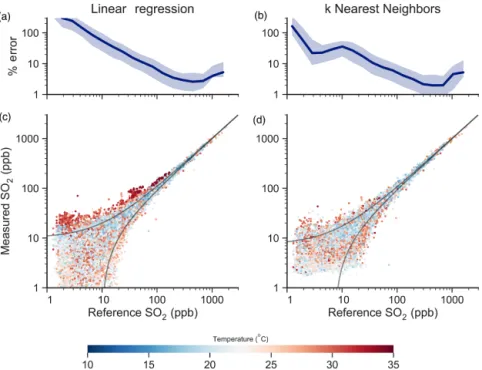
These two approaches (LR and kNN) are evaluated for all sensors by splitting the data into training and validation sub-sets: 70 % of the data were randomly selected for training, and the remaining 30 % for validation throughout the entire data collection period (which varies for each sensor). Pre-dictive power of the models is described by their correlation coefficient (r2), mean absolute error (MAE), and root mean square error (RMSE), evaluated only on the previously un-seen validation data (and not on the training dataset itself). Results for node SO2-02 are presented in Fig. 5.
Figure 5a and c show results from the multivariate linear regression (Eq. 1). SO2mixing ratios measured by the
elec-trochemical sensor are correlated well with the reference SO2
monitor (r2=0.987; 95 % CI: 0.986–0.988) and are reason-ably accurate (RMSE = 9.7 ppb; 95 % CI: 9.6–9.9 ppb). The relative error (as a percentage of absolute concentration) de-creases as the concentration of SO2increases, dropping
be-low 20 % around 50 ppb and bebe-low 5 % at 100 ppb. At the same time, the RMSE increases as the [SO2] range increases,
since small fractional errors lead to large absolute errors at high concentrations. This model performs well at high con-centrations because the VWEresponse (which is linear with
concentration) dominates the signal and is large relative to any shifts in the baseline. However, the LR calibration
per-Figure 4. Box-and-whisker plots showing results from the initial spot-check of various algorithms – linear regression (LR), least absolute shrinkage and selection operator regression (LASSO), ridge regression (RR), classification and regression tree regression (CART), and k nearest neighbors regression (kNN) – to deter-mine their ability to quantify SO2using three independent variables
(VWE, VAE, and T ). Each box represents the interquartile range,
with the whiskers describing the minimum and maximum values. Each algorithm was run on data that were as-is (“unscaled”, blue boxes) and normalized by removing the mean and scaling to unit variance (“scaled”, green boxes). Results shown are for a single sen-sor (SO2-02) covering 145 467 1 min data points.
forms less well at low SO2 concentrations, overestimating
SO2levels when the temperature is highest. Under these
con-ditions the temperature response dominates the sensor signal and, since it is apparently nonlinear, is not captured well by the LR.
Figure 5b and d show results for the kNN model, which offers improved performance over the LR model: the corre-lation coefficient is 0.995 (95 % CI: 0.994–0.995) and the RMSE is 6.3 ppb (95 % CI: 6.2–6.5 ppb). kNN outperforms the linear model at lower SO2concentrations, while
perform-ing similarly at higher concentrations, with the relative error dropping below 20 % at 20 ppb and below 5 % at 100 ppb. Unlike in the LR case, there is no clear relationship between T and measurement bias, indicating that kNN successfully captures the nonlinear temperature response of the sensor. kNN cannot infer the derivative of any feature (T , RH) and thus may be a limitation in cases where environmental con-ditions shift rapidly or for other types of sensors for which derivatives are more important (Masson et al., 2015; Pang et al., 2017).
The results shown in Fig. 5 are for a single sensor node co-located with the Pahala AQ station for the entire study period, but applying these algorithms to results from the other sen-sors (over the time they were located at Pahala) gives qual-itatively similar results. A complete statistical summary of results for all nine sensors can be found in Table 1. Regard-less of the algorithm used, results from the calibrated sen-sors are correlated well to the reference measurements. The few previous studies in which ambient SO2 was measured
Figure 5. Validation results using multivariate linear regression (a, c) and k nearest neighbors regression (b, d). Data are shown as the SO2
measurement by a single sensor (SO2-02) vs. the reference measurement from the AQ station, colored by T . Relative error (a, b) is shown as a function of observed SO2concentration (the interquartile range is shown as the shaded region). Data shown are for the test set only, made
up of 30 % of data collected over the entire measurement period (15 January to 25 April 2017, n = 125 258). Results for other sensors are given in Table 1.
Table 1. Summary of calibration results for all sensors deployed in this study.
Linear regressionb knearest neighborsb Hybrid regressionc Node no. Na MAE RMSE r2 MAE RMSE r2 MAE RMSE r2
(ppb) (ppb) (ppb) (ppb) (ppb) (ppb) SO2-01 44 647 7.5 9.9 0.990 4.1 5.4 0.997 3.6 6.6 0.996 SO2-02 125 258 7.4 9.7 0.987 4.2 6.3 0.995 3.3 6.7 0.994 SO2-03 2505 6.3 9.5 0.998 4.1 9.8 0.998 3.3 7.5 0.999 SO2-04 5382 10.3 15.8 0.989 4.8 11.4 0.995 4.2 10.2 0.996 SO2-05 4469 10.3 13.2 0.992 3.9 7.4 0.998 3.7 7.1 0.998 SO2-06 60 686 7.6 10.2 0.987 3.9 5.6 0.996 3.3 7.0 0.995 SO2-07 5322 4.8 7.1 0.997 2.5 5.1 0.998 2.4 5.1 0.999 SO2-10 5311 9.9 13.7 0.991 4.1 7.1 0.997 3.9 7.8 0.998 SO2-12 1955 6.9 9.7 0.998 3.6 8.8 0.998 3.0 6.7 0.999 Median 7.5 9.9 0.991 4.1 7.1 0.997 3.3 7.0 0.997 SD 1.9 2.7 0.004 0.6 2.2 0.001 0.5 1.4 0.002 aTotal number of 1 min data points, covering only the period during which the sensor was located at the Pahala AQ station for calibration. bUsing the methods described in the text (and shown in Fig. 5) for evaluating node SO2-02.
cSee “Practical Calibration Considerations” subsection for details.
2015) have found little to no correlation to reference data, which is likely due to exceedingly low ambient SO2 levels
in the study regions and the cross sensitivities of the sen-sor to more abundant pollutant species (Lewis et al., 2015). For context, co-location studies of different electrochemical sensors targeting more abundant pollutants have found cor-relations with reference instruments (r2) to range between
0.7 and 0.96 for O3, NO2, NO, and CO (Cross et al., 2017;
Jiao et al., 2016; Mead et al., 2013; Popoola et al., 2016; Zimmerman et al., 2017), with estimates of RMSE spanning 4–60 ppb for O3 (Cross et al., 2017; Sadighi et al., 2017;
Spinelle et al., 2015), 4–22 ppb for NO (Cross et al., 2017; Masson et al., 2015), 39 ppb for CO (Cross et al., 2017), and 4.5 ppb for NO2(Cross et al., 2017) and estimates of MAE of
38 ppb for CO, 3.5 ppb for NO2, and 3.4 ppb for O3
(Zimmer-man et al., 2017). However, it is difficult to directly compare performance metrics (r2, RMSE) obtained from the different calibration algorithms taken in these different studies, given the differences not only in sensor types but in also environ-mental conditions (T , RH, range of pollutant concentrations, and interferences by other pollutants).
3.4 Practical calibration considerations
The results in Fig. 5 and Table 1 show that the kNN regres-sion performs well when the full range of measurement con-ditions (pollutant levels, T ) is covered in the training set. However, training and validating sensors in the same phys-ical location, under similar environmental conditions, is in many ways a best-case scenario and is not always possible for most calibration efforts. Because calibration (co-location) periods are generally limited in time, they likely will not cover the full range of environmental conditions; for exam-ple, they might not cover the highest levels of pollutants, or the full range of temperatures at a given site (which can require months to years of co-located measurements). It is therefore important to understand how such real-world con-straints may affect the accuracy of sensor calibrations.
Figure 6 shows results from the LR and kNN algorithms, trained under subsets of our data to mimic such real-world calibration scenarios. Each row in the diagram represents a different calibration scenario: models were trained on data ranging from 0 to 50 ppb SO2in row one, 0 to 150 ppb SO2
row two, and 0 to 500 ppb SO2row three. After being trained
on the truncated datasets, they were evaluated using the entire previously withheld validation dataset (with the full dynamic range in SO2).
In such limited training-set cases, the LR performs about the same as in the full training-set case (Fig. 5). The only exception is the ≤ 50 ppb condition (row 1), whose calibra-tion lacks the dynamic range for an accurate determinacalibra-tion of sensitivity (c1in Eq. 1). In all cases, performance of LR
at low SO2 concentrations is relatively poor, again due to
the importance of nonlinear temperature effects under these conditions. By contrast, when the SO2 levels in the
train-ing sets are limited, kNN performs poorly when SO2
lev-els in the validation set are high. This is because kNN can-not extrapolate outside the range of data with which it was trained. This is problematic in an area such as Hawai‘i where it is difficult to know the upper bounds of SO2
concentra-tions; similar scenarios may occur in polluted urban areas, where plumes could be intercepted or new sources emerge. Thus, when the full range of pollutant concentrations is not accessed during calibration, each regression technique has a strength and a weakness: LR can extrapolate to higher con-centrations, whereas kNN cannot; but LR does not correct for the temperature dependence of the signal, whereas kNN can.
To preserve the best feature of each approach, we pro-pose a hybrid regression approach using both algorithms in a piece-wise fashion. This hybrid approach entails using kNN below some concentration threshold (here, 50 ppb) and LR when it is above this threshold. Because we are trying to predict the concentration, the determination of whether this threshold is crossed must be made using the sensor mea-surements (VWE, VAE, T ) only. We use a kNN classifier to
make this determination using a method similar to that sug-gested by Kuncheva (2000), thereby classifying each mea-surement as either “above threshold” or “below threshold”. The threshold was chosen by performing a grid search using target SO2concentrations that are included within the
bound-aries of our training dataset; the threshold that produced the lowest RMSE was then chosen as the target threshold moving forward (here, 50 ppb).
Results from the hybrid regression are shown in the right-most column of Fig. 6. It generally performs better (with a lower RMSE) than either of the two regression approaches, as it can correct for the nonlinear temperature dependence at low concentrations, while performing well across the entire dynamic range, even when calibrated under lower-SO2
con-ditions. The hybrid algorithm offers an approach for accu-rately extrapolating to pollutant levels higher than were cov-ered during the calibration period.
3.5 Multiple site validation
The performance of the hybrid regressor provides confidence in the ability to calibrate sensors via co-location and then de-ploy them at a different physical location, an essential step in building any distributed network of sensors. This was tested directly on two nodes (SO2-04, SO2-13) via calibration by co-location at the Pahala AQ station for a period of 48 h (re-sults in Table 1) followed by relocation to the Hilo AQ station (80 km to the northeast; Fig. 1), where they remain in opera-tion as of August 2017. The data collected at Hilo (118 days, n =115 343) were then evaluated using the hybrid regressor trained using data from Pahala.
The results of this evaluation for one of the nodes (SO2-04) are shown in Fig. 7. The calibration carried out at Pa-hala performs well at Hilo (r2=0.892, RMSE = 6.9 ppb); this is only somewhat worse than the performance of a sen-sor (SO2-02) trained at Pahala over the same 2 days and then kept at Pahala for validation on the subsequent 118 days (r2=0.986, RMSE = 9.6 ppb; see Fig. S1).
Measurement error is higher for the sensor relocated in Hilo than the one left at Pahala, largely due to the differ-ences in the training and test environments. As seen in the two probability distribution plots (right side of Fig. 7), the calibration data were from a colder- and higher-SO2
environ-ment (Pahala) than was used in the evaluation (Hilo). Specif-ically, Pahala did not experience any clean air (SO2<1 ppb)
and experienced cooler temperatures, whereas Hilo was most often clean (due to influence from marine air), leading to
Figure 6. Comparing linear regression, k nearest neighbors regression, and hybrid regression on various subsets of the training data by splitting on arbitrary SO2thresholds (row 1: < 50 ppb; row 2: < 150 ppb; row 3: < 500 ppb). All models were validated using the entire SO2
and T ranges of the previously withheld validation dataset.
an imbalance in what the model was trained to perform. Nonetheless, the performance of the sensor and the robust-ness of its calibration at the new site is encouraging. The other node (SO2-13), calibrated in a similar fashion, per-formed comparably (r2=0.880, RMSE = 8.5 ppb). These sensors compare reasonably well to the sensor (SO2-02), which was kept at Pahala and calibrated for only 2 days (Fig. S1); to our knowledge, this is the first demonstration of an electrochemical sensor being trained in one environment and validated in another.
3.6 Measuring SO2at low(er) concentrations
Because of the intensity of the volcanic plume, with SO2
lev-els regularly reaching 100 s (and even 1000 s) of ppb, the dy-namic range of the present measurements is extremely high, with upper-limit concentrations much greater than is typi-cally found for SO2(and other pollutants) in most
environ-ments. Assessing sensor performance at lower SO2
concen-trations is thus important for understanding the potential for
sensors and calibration algorithms to be used under a wider range of conditions. Sensor performance under lower-SO2
conditions can be evaluated using the present dataset by re-moving all points in which the reference value was greater than some threshold value (chosen here to be 25 ppb SO2,
a reasonable value for cities in India and China; Meng et al., 2010; O’Shea et al., 2016).
Figure 8 shows kNN regression results for node SO2-02 under lower-SO2conditions only; these were generated using
the same technique for generating Fig. 5, but with the training and validation sets limited only to reference SO2
measure-ments < 25 ppb. In addition, we found the marginal variance caused by relative humidity was non-negligible when con-sidering measurements at these low concentrations, and thus RH was added as an input to the kNN model. Sensor perfor-mance remains good in this case, with an RMSE of 2.9 ppb and r2of 0.788; even between 3 and 25 ppb, relative errors are ∼ 20 %. Across all nine sensors, performance is similar, with a median RMSE of 2.2 (±0.6) ppb and an r2of 0.864 (±0.061) (see Table S1).
Figure 7. Hybrid regression results for node SO2-04 when trained using data from the Pahala AQ station (2 days) and validated using data from the Hilo AQ station (4 months). Right panel: kernel density estimates showing the distribution of temperature and SO2used both in the
training (Pahala) and validation (Hilo) datasets. The difference in the environmental conditions is likely the cause of the somewhat decreased performance of the sensor calibration at the new site. For comparison, a plot comparing a different sensor (SO2-02) which was trained during these same 2 days and then re-evaluated at the same physical site is shown in Fig. S1 in the Supplement.
Figure 8. Performance of the sensor (node SO2-02) at lower (< 25 ppb) levels of SO2, evaluated using kNN regression. Data shown
are from the validation dataset and result in an r2=0.788 with RMSE = 2.9 ppb. The top plot shows the relative error as a percent-age of concentration where the dark line is the median value and the shaded region is the interquartile range. Other sensors evaluated at 0–25 ppb showed even better performance (median r2: 0.864; me-dian RMSE: 2.1 ppb); results are given in Table S1.
The kNN approach works well when trained on lower-concentration data because it can sufficiently map the non-linear temperature and relative humidity dependence with-out needing to determine the functional form of the equation. The improved performance (lower RMSE) of this assessment compared to that of the full dataset (Fig. 5, Table 1) is a re-sult of removing the highest-SO2 points, which contribute
substantially to absolute error. Overall, this robust sensor cal-ibration at lower SO2levels suggests that the sensor
calibra-tion approach described here is not limited just to the present environment (which is characterized by very high SO2
lev-els) and could be applied to a wider range of conditions (e.g., polluted urban areas) as well.
3.7 Drift in sensitivity over time
The rate of drift in sensor sensitivity (change in gain) over time is a crucial parameter in sensor characterization, as it determines the interval of calibration, as well as the overall useable lifetime of the sensors. Recent work has shown vary-ing rates of drift, rangvary-ing from several days (Smith et al., 2017) to many months (Mead et al., 2013; Popoola et al., 2016). We expect to observe a gradual degradation in sensi-tivity over time as the electrolyte evaporates; the manufac-turer (Alphasense Ltd.) quotes a 50 % decay over 2 years. The long duration of the data collection period (4.5 months)
Figure 9. Sensitivity decay for a single SO2-B4 sensor (SO2-02) across 18 weeks. After being trained on data from weeks 2 to 3, the sensor was evaluated using the hybrid regression approach for each successive week of data and fit using ordinary least-squares regression. Slope indicates whether the model was underpredicting (m < 1) or overpredicting (m > 1) SO2values. A decrease in sensitivity would be seen as
a gradual decline in the slope, which is not seen here. Light blue points (weeks 17–21) denote periods during which the RHT sensor was behaving erratically, limiting the amount of useful trusted data.
enables us to determine the SO2sensor drift in the present
dataset.
To determine the time-dependent change in sensitivity of the electrochemical sensor to its target gas, we perform a LR of the predicted mixing ratios (using the hybrid regression method) against the reference data collected at the AQ sta-tion. The hybrid regressor was trained using data from weeks 2 to 3 (10 days total) and then evaluated on all subsequent data. Figure 9 shows the comparison between the calibrated sensor measurements and reference values of SO2for each
week. The slope is ∼ 1 throughout the first 18 weeks after deployment (weeks 4–21) without significant degradation in sensitivity to SO2. The last 5 weeks of data (shown in light
blue) should be treated with caution, as the temperature sen-sor used in the device began to behave erratically, includ-ing periods where the temperature sensor reported anoma-lously high values (> 40◦C; all such data points were
ex-cluded from this analysis). Over this 4-month period, there is no evidence for a gradual decay in sensitivity, which would suggest the evaporation of the electrolyte solution. This in-dicates that under the present environmental conditions, the SO2sensor calibration remains stable over a period of at least
4 months, with no need for re-calibration over this time.
4 Implications and future work
In this work, we have laid out a general calibration approach for electrochemical sensors based on co-location with refer-ence (regulatory-grade) monitors. This work shows that the complex temperature dependence of electrochemical sensors can be accounted for using nonparametric regression tech-niques. To overcome the limitations of nonparametric meth-ods, we introduced a new hybrid linear–nonparametric gression scheme that provides the benefits of multiple re-gression techniques simultaneously and allows for the use of electrochemical sensors in environments for which they have not been previously calibrated against. This hybrid approach enables reliable long-term measurements of SO2across a
dy-namic range of 1 ppb to 2 ppm with good accuracy (RMSE < 7 ppb) and correlation (r2>0.99) with the reference moni-tor. Additionally, we have shown that low-cost electrochemi-cal SO2sensors can provide acceptable results in lower-SO2
environments, extending their utility to other locales, and that they exhibit little to no sign of sensitivity decay through the first 18 weeks of deployment, suggesting the necessary re-calibration interval is on the order of several months (as op-posed to weeks or days).
Ideally, calibration by co-location with reference monitors will cover the entire range of conditions (e.g., pollutant lev-els, temperature) expected to be encountered; however, this is not always possible, especially when using sensors in pre-viously unmeasured conditions and geographic areas. When
deciding how large a training dataset is needed, the key quan-tity to consider is the fraction of total feature space mapped, rather than total number of measurements taken (or time cal-ibrated). In the present study (which uses the Alphasense SO2-B4 sensor on the island of Hawai‘i), this means com-pletely covering the 2-D vector space of SO2 concentration
and temperature; for other sensors in other environments, the feature space likely also should include concentrations of rel-evant cross-sensitive species, such as nitrogen dioxide in the case of ozone sensors (Mueller et al., 2017; Spinelle et al., 2015). Under conditions in which environmental conditions (T or RH) change very rapidly, the feature space may include the time derivative of these as well (Masson et al., 2015; Pang et al., 2017).
The scope of this work is limited to the measurement of a single pollutant (SO2) by a single make of sensor
(Al-phasense SO2-B4) in a single environment (characterized by a very wide range in SO2concentrations, low levels of other
pollutants, and relatively little variability in T ). It is there-fore difficult to generalize the specific results of this work to other pollutants, sensors, and environments. However, the general approaches discussed here – the use of a hybrid linear–nonparametric regression algorithm, the examination of calibrations by limiting the environmental conditions of the training set, and the testing of sensors and algorithms by calibration at one reference site and validation at another – could be applied to other sensor system as well; sensor char-acterization in these other conditions is an important area of future research. Such characterization efforts, covering a full range of pollutants (e.g., CO, O3, NO, NO2) and
environ-ments (with different pollutant levels, temperature and hu-midity conditions, etc.) will improve our understanding of the performance and applicability of low-cost AQ sensors for a range of studies in AQ, human health, and atmospheric chemistry.
Data availability. All data can be provided by the author upon re-quest.
The Supplement related to this article is available online at https://doi.org/10.5194/amt-11-315-2018-supplement.
Competing interests. The authors declare that they have no conflict of interest.
Disclaimer. The views expressed in this document are solely those of the authors and do not necessarily reflect those of the Agency. EPA does not endorse any products or commercial services men-tioned in this work.
Acknowledgements. The authors are grateful to Steven Wofsy for helpful advice related to data analysis, William Porter for help with commonality analysis, John Saffell for helpful comments and ad-vice, and the members of TREX 2015 (Michael Chen, Jennifer Murphy, Alexandra Tevlin, Katherine Adler, Bridget Bassi, Josefin Betsholtz, Kali Benavides, Maria Cassidy, Mary Cunha, Kather-ine Dieppa, Samatha Harper, Samantha Hartzell, Teresa Hegarty, Julia Hogroian, Holly Josephs, Julia Longmate, Kendrick Many-mules, Rucha Mehendale, Amanda Parry, Erin Reynolds, Emily Shorin, Brenda Stern, Shanasia Sylman, Tiffany Wang, Siyi Zhang), TREX 2016 (Christopher Lim, Jillian Dressler, Rachel Galowich, Francesca Majluf, Alexandra Radway, Kali Rosendo, Rebecca Sug-rue, George Varnavides), and TREX 2017 (Jon Kaneshiro, Chelsea Chitty, Deanna Delgado, Lilian Dove, Abigail Harvey, Danielle Hecht, Alexa Jaeger, William Moses, Mikayla Murphy, Daniel Richman, Tchelet Segev, Amber VanHemel) for assistance in con-struction and installation of the sensors.
Funding for this project was provided by MIT’s Department of Civil and Environmental Engineering, the MIT Tata Center for Technology and Design, and the US Environmental Protection Agency under grant RD-83618301. It has not been formally re-viewed by the EPA. Gabriel Isaacman-VanWertz was supported by the National Science Foundation Postdoctoral Research Fellowship (AGS-PRF1433432).
Edited by: Hendrik Fuchs
Reviewed by: two anonymous referees
References
Altman, N. S.: An introduction to kernel and nearest-neighbor nonparametric regression, Am. Stat., 46, 175–185, https://doi.org/10.1080/00031305.1992.10475879, 1992. Breiman, L.: Bagging predictors, Mach. Learn., 24, 123–140,
https://doi.org/10.1007/BF00058655, 1996.
Breiman, L., Friedman, J. H., Olshen, R. A., and Stone, C. J.: Clas-sification and Regression Trees, Wadsworth & Brooks/Cole Ad-vanced Books & Software, Monterey, CA, USA, 1984.
Cao, Z., Buttner, W. J., and Stetter, J. R.: The properties and appli-cations of amperometric gas sensors, Electroanal., 4, 253–266, https://doi.org/10.1002/elan.1140040302, 1992.
Castell, N., Dauge, F. R., Schneider, P., Vogt, M., Lerner, U., Fishbain, B., Broday, D., and Bartonova, A.: Can commer-cial low-cost sensor platforms contribute to air quality mon-itoring and exposure estimates?, Environ. Int., 99, 293–302, https://doi.org/10.1016/j.envint.2016.12.007, 2017.
Cross, E. S., Williams, L. R., Lewis, D. K., Magoon, G. R., Onasch, T. B., Kaminsky, M. L., Worsnop, D. R., and Jayne, J. T.: Use of electrochemical sensors for measurement of air pollution: cor-recting interference response and validating measurements, At-mos. Meas. Tech., 10, 3575–3588, https://doi.org/10.5194/amt-10-3575-2017, 2017.
Edmonds, M., Sides, I. R., Swanson, D. A., Werner, C., Mar-tin, R. S., Mather, T. A., Herd, R. A., Jones, R. L., Mead, M. I., Sawyer, G., Roberts, T. J., Sutton, A. J., and Elias, T.: Magma storage, transport and degassing during the 2008–10 summit eruption at Kilauea Volcano, Hawai‘i, Geochim. Cosmochim.
https://doi.org/10.5194/amt-9-5281-2016, 2016.
Knapp, C. H. and Carter, G. C.: The generalized correlation method for estimation of time delay, IEEE T. Acoust. Speech., 24, 320– 327, https://doi.org/10.1109/TASSP.1976.1162830, 1976. Kohavi, R.: A study of cross-validation and bootstrap for accuracy
estimation and model selection, Appear. Int. Jt. Conf. Articial Intell., 5, 1–7, 1995.
Kroll, J. H., Cross, E. S., Hunter, J. F., Pai, S., Wal-lace, L. M. M., Croteau, P. L., Jayne, J. T., Worsnop, D. R., Heald, C. L., Murphy, J. G., and Frankel, S. L.: Atmo-spheric evolution of sulfur emissions from K¯ılauea: real-time measurements of oxidation, dilution, and neutralization within a volcanic plume, Environ. Sci. Technol., 49, 4129–4137, https://doi.org/10.1021/es506119x, 2015.
Kuncheva, L. I.: Clustering-and-selection model for classifier com-bination, KES’2000. Fourth Int. Conf. Knowledge-Based In-tell. Eng. Syst. Allied Technol. Proc. (Cat. No.00TH8516), 30 August–1 September 2000, Brighton, UK, vol. 1, 185–188, https://doi.org/10.1109/KES.2000.885788, 2000.
Lewis, A. and Edwards, P.: Validate personal air-pollution sensors, Nature, 535, 29–31, https://doi.org/10.1038/535029a, 2016. Lewis, A. C., Lee, J. D., Edwards, P. M., Shaw, M. D., Evans, M. J.,
Moller, S. J., Smith, K. R., Ellis, M., Gillott, S., White, A. A., Buckley, J. W., Ellis, M., Gillot, S. R., and White, A. A.: Evaluating the performance of low cost chemical sensors for air pollution research, Faraday Discuss., 189, 85–103, https://doi.org/10.1039/C5FD00201J, 2015.
Longo, B. M.: The K¯ılauea Volcano Adult Health Study, Nurs. Res., 58, 23–31, https://doi.org/10.1097/NNR.0b013e3181900cc5, 2009.
Longo, B. M.: Adverse health effects associated with in-creased activity at K¯ılauea Volcano: a repeated population-based survey, edited by: Béria, J. U., Spickett, J., Szadkowska-Stanczyk, I., ISRN Public Heal., 2013, 1–10, 475962, https://doi.org/10.1155/2013/475962, 2013.
Longo, B. M. and Yang, W.: Acute bronchitis and volcanic air pollution: a community-based cohort study at K¯ılauea Vol-cano, Hawai‘i, USA, J. Toxicol. Env. Heal. A, 71, 1565–1571, https://doi.org/10.1080/15287390802414117, 2008.
Longo, B. M., Yang, W., Green, J. B., Crosby, F. L., and Crosby, V. L.: Acute health effects associated with exposure to volcanic air pollution (vog) from increased activity at
Ki-Saffell, J. R., and Jones, R. L.: The use of electro-chemical sensors for monitoring urban air quality in low-cost, high-density networks, Atmos. Environ., 70, 186–203, https://doi.org/10.1016/j.atmosenv.2012.11.060, 2013.
Meng, Z. Y., Xu, X.-B., Wang, T., Zhang, X. Y., Yu, X. L., Wang, S. F., Lin, W. L., Chen, Y. Z., Jiang, Y. A., and An, X. Q.: Ambient sulfur dioxide, nitrogen diox-ide, and ammonia at ten background and rural sites in China during 2007–2008, Atmos. Environ., 44, 2625–2631, https://doi.org/10.1016/j.atmosenv.2010.04.008, 2010.
Mueller, M., Meyer, J., and Hueglin, C.: Design of an ozone and nitrogen dioxide sensor unit and its long-term operation within a sensor network in the city of Zurich, Atmos. Meas. Tech., 10, 3783–3799, https://doi.org/10.5194/amt-10-3783-2017, 2017. O’Shea, P. M., Sen Roy, S., and Singh, R. B.: Diurnal variations in
the spatial patterns of air pollution across Delhi, Theor. Appl. Cli-matol., 124, 609–620, https://doi.org/10.1007/s00704-015-1441-y, 2016.
Pang, X., Shaw, M. D., Lewis, A. C., Carpenter, L. J., and Batchel-lier, T.: Electrochemical ozone sensors: a miniaturised alter-native for ozone measurements in laboratory experiments and air-quality monitoring, Sensor. Actuat. B-Chem., 240, 829–837, https://doi.org/10.1016/j.snb.2016.09.020, 2017.
Pedregosa, F., Varoquaux, G., Gramfort, A., Michel, V., Thirion, B., Grisel, O., Blondel, M., Louppe, G., Prettenhofer, P., Weiss, R., Dubourg, V., Vanderplas, J., Passos, A., Cournapeau, D., Brucher, M., Perrot, M., and Duchesnay, É.: Scikit-learn: ma-chine learning in python, J. Mach. Learn. Res., 12, 2825–2830, 2012.
Piedrahita, R., Xiang, Y., Masson, N., Ortega, J., Collier, A., Jiang, Y., Li, K., Dick, R. P., Lv, Q., Hannigan, M., and Shang, L.: The next generation of low-cost personal air quality sensors for quan-titative exposure monitoring, Atmos. Meas. Tech., 7, 3325–3336, https://doi.org/10.5194/amt-7-3325-2014, 2014.
Popoola, O. A. M., Stewart, G. B., Mead, M. I., and Jones, R. L.: Development of a baseline temperature-correction methodol-ogy for electrochemical sensors, and implications of this cor-rection on long-term stability, Atmos. Environ., 147, 330–343, https://doi.org/10.1016/j.atmosenv.2016.10.024, 2016.
Rifkin, R.: Notes on regularized least squares, Massachusetts Inst. Technol., available at: http://cbcl.mit.edu/publications/ps/ MIT-CSAIL-TR-2007-025.pdf (last access: 12 January 2018), 2007.
Roberts, T. J., Braban, C. F., Oppenheimer, C., Martin, R. S., Fresh-water, R. A., and Dawson, D. H.: Electrochemical sensing of vol-canic gases, Chem. Geol., 333, 74–91, 2012.
Sadighi, K., Coffey, E., Polidori, A., Feenstra, B., Lv, Q., Henze, D. K., and Hannigan, M.: Intra-urban spatial variability of sur-face ozone and carbon dioxide in Riverside, CA: viability and validation of low-cost sensors, Atmos. Meas. Tech. Discuss., https://doi.org/10.5194/amt-2017-183, in review, 2017. Seibold, D. R. and McPhee, R. D.: Commonality analysis:
a method for decomposing explained variance in multi-ple regression analyses, Hum. Commun. Res., 5, 355–365, https://doi.org/10.1111/j.1468-2958.1979.tb00649.x, 1979. Smith, K., Edwards, P. M., Evans, M. J. J., Lee, J. D.,
Shaw, M. D., Squires, F., Wilde, S., and Lewis, A. C.: Clus-tering approaches that improve the reproducibility of low-cost air pollution sensors, Faraday Discuss., 200, 621–637, https://doi.org/10.1039/C7FD00020K, 2017.
Snyder, E. G., Watkins, T. H., Solomon, P. A., Thoma, E. D., Williams, R. W., Hagler, G. S. W., Shelow, D., Hindin, D. A., Kilaru, V. J., and Preuss, P. W.: The changing paradigm of air pollution monitoring., Environ. Sci. Technol., 47, 11369–77, https://doi.org/10.1021/es4022602, 2013.
Spinelle, L., Gerboles, M., Villani, M. G., Aleixan-dre, M., and Bonavitacola, F.: Calibration of a cluster of low-cost sensors for the measurement of air pollu-tion in ambient air, Proc. IEEE Sensors, 2014, 21–24, https://doi.org/10.1109/ICSENS.2014.6984922, 2014.
Spinelle, L., Gerboles, M., Villani, M. G., Aleixandre, M., and Bonavitacola, F.: Field calibration of a cluster of low-cost available sensors for air quality monitoring. Part A: Ozone and nitrogen dioxide, Sensor. Actuat. B-Chem., 215, 249–257, https://doi.org/10.1016/j.snb.2015.03.031, 2015.
Tam, E., Miike, R., Labrenz, S., Sutton, A. J., Elias, T., Davis, J., Chen, Y.-L., Tantisira, K., Dockery, D., and Avol, E.: Volcanic air pollution over the Island of Hawai‘i: Emissions, dispersal, and composition. Association with respiratory symptoms and lung function in Hawai‘i Island school children, Environ. Int., 92–93, 543–552, https://doi.org/10.1016/j.envint.2016.03.025, 2016. Tibshirani, R.: Regression selection and shrinkage via the lasso, J.
R. Stat. Soc. B, 58, 267–288, 1996.
US EPA: EPA AirNow, available at: https://airnow.gov/, last access: 3 August 2017.
Van Der Walt, S., Colbert, S. C., and Varoquaux, G.: The NumPy ar-ray: a structure for efficient numerical computation, Comput. Sci. Eng., 13, 22–30, https://doi.org/10.1109/MCSE.2011.37, 2011. Waskom, M., Botvinnik, O., O’Kane, D., Hobson, P., Lukauskas, S.,
Gemperline, D. C., Augspurger, T., Halchenko, Y., Cole, J. B., Warmenhoven, J., Ruiter, J. De, Hoyer, S., Vanderplas, J., Villalba, S., Kunter, G., Quintero, E., Bachant, P., Mar-tin, M., Meyer, K., Miles, A., Ram, Y., Pye, C., Yarkoni, T., Williams, M. L., Evans, C., Fitzgerald, C., Brian, Fonnes-beck, C., Lee, A., and Qalieh, A.: Mwaskom/Seaborn: V0.8.0 (July 2017), https://doi.org/10.5281/zenodo.824567, 2017. White, R. M., Paprotny, I., Doering, F., Cascio, W. E.,
Solomon, P. A., and Gundel, L. A.: Sensors and apps for community-based atmospheric monitoring, EM Air Waste Manag. Assoc. Mag. Environ. Manag., May, Pittsburgh, PA, USA, 36–40, 2012.
Zimmerman, N., Presto, A. A., Kumar, S. P. N., Gu, J., Hau-ryliuk, A., Robinson, E. S., Robinson, A. L., and Sub-ramanian, R.: Closing the gap on lower cost air quality monitoring: machine learning calibration models to improve low-cost sensor performance, Atmos. Meas. Tech. Discuss., https://doi.org/10.5194/amt-2017-260, in review, 2017.