Characterizing electrodermal responses during sleep in a 30-day ambulatory study

by

Sara Ann Taylor

B.Sc., Brigham Young University, 2014

Submitted to the Program in Media Arts and Sciences, School of Architecture and Planning,

in Partial Fulfillment of the Requirements for the Degree of

Masters of Science in Media Arts and Sciences at the

Massachusetts Institute of Technology September 2016

MASAHU S INSTTUTE OF TECHNOLGY

LIBRARIES

ARCHIEV'L

@ 2016 Massachusetts Institute of Technology. All rights reserved.

Signature of Author

Signature redacted

Program in Media Arts and Sciences August 5, 2016

Certified by

Signature redacted

Rosalind W. Picard Professor of Media Arts and Sciences

Signature redacted

Accepted by

7 V

Pattie Maes Academic Head, Program in Media Arts and Sciences

Characterizing Electrodermal Responses during Sleep in a 30-day Ambulatory Study

by

Sara Ann Taylor

B.Sc., Brigham Young University, 2014

Submitted to the Program in Media Arts and Sciences, School of Architecture and Planning,

on August 5, 2016

in Partial Fulfillment of the Requirements for the Degree of Masters of Science in Media Arts and Sciences

at the

Massachusetts Institute of Technology

ABSTRACT

Electrodermal activity (EDA) refers to the electrical activity measured on and under the surface of the skin and has been used to study sleep, stress, and mood. While gathering this signal was once confined to the laboratory, it can now be acquired in ambulatory studies through commercially available wearable sensors. In this thesis, we model and analyze electrodermal response (EDR) events (1-5 second peaks in the EDA signal) during sleep in an ambulatory study.

In particular, we describe an EDR event detection algorithm and extract shape features from these events to discuss the difference in shape between sleep and wake. We also de-scribe an automatic artifact detection algorithm that we use on over 100,000 hours of EDA data we have collected in the 30-day SNAPSHOT Study from 164 participants. Finally, we model the detected EDR events as a point process using a state-space generalized linear model. We identify a significant influence of recent EDR event history on current EDR event likelihood across different participants. We also use this model to analyze EDR event rates during different periods of the night.

Thesis Supervisor: Rosalind W. Picard Title: Professor of Media Arts and Sciences

Characterizing Electrodermal Responses during Sleep in a 30-day Ambulatory Study by

Sara Ann Taylor

B.Sc., Brigham Young University, 2014

Advisor

Signature redacted

Dr. Rosalind W. Picard Professor of Media Arts and Sciences MIT Media Lab

Reader

redactd_________

Dr. Emery N. Brown Edward Hood Taplin Professor of Medical Engineering Professor of Computational Neuroscience Warren M. Zapol Professor of Anaesthesia

Massachusetts Institute of Technology

Signature redacted

Reader

Dr. Pattie Maes Professor of Media Arts and Sciences MIT Media Lab

Contents

2.2.5 Wearables . . . . 15 . . . . 1 5 . . . . 17 . . . . 1 7 . . . . 17 . . . 2 1 . . . 2 2 . . . 2 2 3 Electrodermal Activity Data

3.1 Background . . . . 3.2 Electrodermal Response (EDR) Event Detection . 3.3 Electrodermal Response Features . . . . 4 Artifact Detection

4.1 Introduction . . . . 4.2 Automatic Identification of Artifacts in Electrodermal Activity Data 4.3 Active Learning for Electrodermal Activity Classification . . . .

27 . . 27 28 29 33 33 . . 34 35

5 Point Process Modeling

3 9 10 11 13 37

5.1 5.2

Background . . . . State-Space Generalized Linear Model . . . . 5.2.1 Observation Equation . . . . 5.2.2 State Equation . . . .

5.2.3 Estimation of Model Parameters using Expectation Maximization

5.2.4 Goodness-of-Fit . . . . 5.2.5 Model Selection . . . . 5.2.6 Special Cases of the State-Space Generalized Linear Model . . . 5.3 Modeling EDR events during sleep . . . .

5.4 R esults . . . . 5.4.1 Selected Models . . . . 5.4.2 Model Fit on Held-out Data . . . . 5.4.3 History Effects . . . . 5.4.4 Time Since Sleep Onset Results . . . . 5.5 Summary . . . . 6 Conclusions and Future Work

6.1 Summary of Work . . . . 6.2 Im plications . . . . 6.3 Future Work . . . . A Automatic Identification of Artifacts in Electrodermal Activity Data B Active Learning for Electrodermal Activity Classification

C State-Space Generalized Linear Model Derivation C. 1 Model Set-up . . . .

C. 1.1 Definitions of Variables . . . . C. 1.2 Observation Equation -Conditional Intensity C.1.3 State Equation . . . . C.2 Expectation-Maximization . . . . C.2.1 Complete Data Likelihood . . . . C.2.2 E-Step . . . . C.2.3 M-Step . . . . C.2.4 EM Algorithm Summary . . . . Function (CIF) 8 37 38 38 40 41 41 42 42 43 49 49 51 54 54 57 61 61 62 63 65 71 79 79 79 80 81 81 81 82 90 96 97 Bibliography

List of Figures

Number of Participants in Each Cohort . . . . Number of Participants in Each Year in School . . . . Distribution of Stress and Anxiety Measures . . . . Distribution of Pre-study MCS Scores and Change in MCS Scores . Distribution of Daily Self-reported Wellbeing Measures . . . . Distribution of Self-Reported Daily Behaviors . . . . Distribution of DLMO . . . . Distribution of Average Time Spent with Phone Screen On per Hour Figure 2.9 Distribution of Self-Reported Sleep Accuracy .

Figure 2.10 Distribution of Sleep Regularity Scores . . . . Figure 2.11 Example of Q-Sensor Data . . . . Figure 3.1 Figure 3.2 Figure 3.3 Figure 3.4 Figure 5.1 Figure 5.2 Figure 5.3 Figure 5.4 Typical EDR . . . .

Example of Identified EDRs . . . . Labeled EDR Features . . . . Comparison of Sleep and Wake EDR Features Example of Detected Artifacts During Sleep Example of Detected Artifacts During Wake EDR Sleep Raster Plot . . . . Histogram of Inter-event Interval (IEI) Times .

Figure 5.5 Distribution of Median of Percentage of Artifact-fl

16 16 18 19 20 21 22 23 24 24 25 28 29 30 31 . . . 44 . . . . 44 . . . . 45 . . . . 46 ree Data . . . . 46 Figure 5.6 Distribution of Number of Sleep Episodes with No Detected Peaks

Figure 5.7 Held-out K-S Statistic for Static-GLM models . . . . Figure 5.8 Held-out K-S Statistic for SS-GLM models . . . . Figure 5.9 Connection between Sleep Regularity and K-S Statistic in SS-GLM Figure 5.10 History Parameters . . . . Figure 5.11 Time Since Sleep Onset Effect for Two Participants . . . . Figure 5.12 Example of Rate Differences and Self-reported Health . . . .

47 52 53 54 55 59 60

10

List of Tables

Table 3.1 Computed EDR Feature Values . . . . 30

Table 5.1 Selected PSTH Models using Minimum AIC Score . . . 49

Table 5.2 Selected Static GLM Models using Minimum AIC Score . . . . 50

Table 5.3 Selected SS-GLM Models using Minimum AIC Score . . . . 50

Table 5.4 Comparing Models using AIC and Goodness-of-Fit Metrics . . . . 51

Table 5.5 Model Ranking based on AIC and K-S Statistic . . . . 51

Table 5.6 Final Selected SS-GLM Models to be Analyzed for Inference . . . . . 55

ACKNOWLEDGEMENTS

I would first like to thank Roz for her willingness to give me space to explore and for encouraging me to solve hard problems. I would also like to thank my readers, Emery Brown and Pattie Maes for their helpful feedback.

To the Affective Computing Group (Asma, Natasha, Vincent, Daniel, Ehi, Kristy, Craig, Grace, Karthik, Akane, Javier, Szymon, Yadid, and Micah): thank you for helping me improve my research and encouraging me to work on exciting problems.

Extra special thanks is due to Akane Sano for allowing me to collaborate with her on the SNAPSHOT study. Additionally, I express my gratitude to Natasha Jaques for pushing us to work on exciting projects and to Yadid Ayzenberg for help in using Tributary to speed up the analysis.

I have also had the pleasure to work with many UROP students (Ian, Marisa, Victo-ria, Yuna, Tim, Sienna, Sarah, Lars, Noah, Kevin, Hank, William, Margaret, and Alicia), whose contributions have not gone unnoticed. And to the Brigham and Women's Hospital, Harvard, and the Macro Connection teams, the SNAPSHOT Study could not have been conducted without your help: thank you!

A big thank you goes to my family, and especially my parents, for their love, support, and encouragement.

And finally, to my best friend and husband, Cameron: thank you for your loving support and willingness to go on this adventure with me.

Chapter 1

Introduction

Many clinical studies have shown how sleep affects us physiologically, mentally, and emo-tionally, and how different behaviors influence sleep; however, these studies are usually conducted in sleep labs with many devices and sensors that inhibit natural sleeping behav-iors. Additionally, these studies are usually conducted in carefully controlled environments. While these studies have helped us begin to understand the role of sleep in humans, they are not directly applicable to everyday life without further research because of the limits that a sleep lab places on natural sleep and behaviors. However, with the rise of smartphones and wearable physiological sensors, researchers now have the tools to objectively measure sleep and behaviors during daily life.

One such physiological measure that can be used to monitor both sleep and wake is electrodermal activity. Electrodermal activity (EDA) refers to the electrical activity mea-sured on and under the surface of the skin [7]. EDA has frequently been used in studies related to affective phenomena and stress because EDA tends to increase as the body re-sponds to arousal or exertion (e.g., [20, 21, 26, 27, 34, 36, 44]). In addition, increases in EDA have also been observed during sleep when arousal and exertion are typically low. In particular, it has been shown that if "sleep storms" (the pattern of many successive elec-trodermal responses during sleep) are present they usually occur during slow-wave sleep [25, 28].

In this thesis, we will model electrodermal response (EDR) events (peaks in the EDA data that are short in duration) in both their shape and their rate patterns during sleep at home. In particular, we will describe an EDR event detection algorithm, how we extract shape features from each event, and how we analyze the shape feature differences during wake and sleep. In order to do so, we also needed to develop an automatic artifact detection algorithm. Additionally, we describe how EDR events can be represented as a temporal

14

point process, a random process composed of a series of binary events in a time-series [14]. We use the point process model described by Czanner et. al. [13] to estimate the rate of EDR events during sleep and use the result to model the relationship between self-reported wellbeing and EDR event rates during sleep. In order to model these patterns and relationships, we use data collected from the ongoing SNAPSHOT Study.

Outline

Chapter 2: SNAPSHOT Study gives details on the study and presents information about the population. The remainder of this thesis is based on data collected during this study.

Chapter 3: Electrodermal Activity Data gives background information on electroder-mal activity and describes a new technique for identifying electroderelectroder-mal responses (EDRs). This technique is used to extract shape features for EDRs throughout the day, and sleep and wake EDR shape features are compared.

Chapter 4: Artifact Detection describes the importance of automatically detecting artifacts in EDA data and describes our machine learning methods to do so.

Chapter 5: Point Process Modeling describes a state-space based generalized linear model that can be used to estimate the rate of a point process such as EDR events during sleep. We then describe how the model is fit to EDA data during sleep for each SNAPSHOT participant. From this model, we draw conclusions about the effect of recent history and time since sleep onset on the rate of EDR events during sleep.

Chapter 6: Conclusions and Future Work summarizes the thesis and implications of the results. We also touch on future work to improve upon the methods presented here.

Chapter 2

SNAPSHOT Study

2.1

General Background

The SNAPSHOT Study is a large-scale and long-term study' that seeks to measure: Sleep, Networks, Affect, Performance, Stress, and Health using Objective Techniques. This study

investigates:

1. how daily behaviors influence sleep, stress, mood, and other wellbeing-related factors 2. how accurately we can recognize/predict stress, mood and wellbeing

3. how interactions in a social network influence sleep behaviors

To date, approximately 250 undergraduate students have participated in the 30-day ob-servational study that collects data from a variety of sources [35]. These students were recruited as socially connected groups with about 40-50 students participating during each of the 6 cohorts since 20132. This study is an NIH-funded collaborative research project3 between the Affective Computing group at the MIT Media Lab and Brigham and Women's Hospital. The Massachusetts Institute of Technology Committee On the Use of Humans as Experimental Subjects (COUHES) approved this study and all participants gave informed consent.

In this thesis, we will present results based on the first 4 cohorts only which had a total of 164 participants since the latter two cohorts were conducted as the analysis was being run (see Figure 2.1 for the number of participants that participated in at least some aspect of

'More details and data visualizations can be found at http: //snapshot .me dia. mit. edu/

2

Note: The first cohort only contained 20 students

3

16

the 30-day SNAPSHOT Study). Participants were all undergraduates, but were distributed across all four years of school with freshman being the highest represented group (see Figure 2.2). Our population was overwhelmingly male (104 participants).

50, 4-d C (U 4-0 E z 40- 30- 20- 10-0

rai zu . Spring 2014 Fall 2014 Spring 2015 Cohort

Figure 2.1: Number of Participants in Each Cohort. during one cohorts wer (U 0. E =3 a- 50- 40- 30- 20-10 0

Each participant only participated cohort. Fall cohorts were conducted in October and November and spring e conducted in February and March.

i-resnman Sophomore

Year in School

Figure 2.2: Number of Participants in Each Year in School

2.2

Data Sources

2.2.1

Standardized Surveys

After being informed of the study protocol and providing consent, participants completed several standardized surveys, including Pittsburg Sleep Quality Index test, Myers Brigg Personality test, Big Five Inventory Personality Test, Morningness-Eveningness question-naire, Perceived Stress Scale, SF-12 survey, and a demographics survey that collected in-formation on age, gender, academic year, academic major, and living situation.

At the end of the 30-day study, participants completed several other post-study surveys, including academic performance during the semester (GPA), Perceived Stress Scale (PSS), SF-12 survey (which gives Physical Component Summary (PCS) and Mental Component Summary (MCS) scores), and the State-Trait Anxiety Index (STAI). See Figure 2.3 for distributions of three of the standardized surveys about stress and anxiety.

We are particularly interested in the Mental Component Summary (MCS) score because of the importance of mental health in overall wellbeing. Figure 2.4 shows the distribution of pre-study MCS scores and the change in MCS scores over the 30-day study (computed as A = post MCS-pre MCS).

2.2.2

Daily Surveys

Each morning (at 8am) and each evening (at 8pm) during the study, participants were emailed a link to an online survey that they were instructed to complete right after waking and right before retiring to bed, respectively. Each participant's survey response was looked over by a member of the research staff to catch any errors or missing entries. Participants were give 36 hours to start the survey and 72 hours to correct any mistakes after the survey was initially emailed.

The morning survey included questions about the participant's sleep, including the time the participant tried to go to bed, sleep latency, wake time, the timing and duration of each awakening or arousal during sleep, and the timing and duration of any naps. Finally, participants rated how they were feeling by adjusting sliders between the following pairs

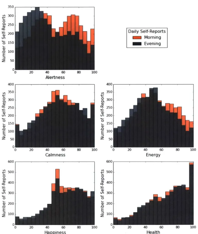
of words: Sleepy - Alert; Sad - Happy; Sluggish - Energetic; Sick - Healthy; and Stressed Out - Calm Relaxed. The slider responses were reported on a scale from 0-100, but participants could not see the numerical value when reporting. Each participant also reported how they were feeling during the evening survey using the same five sliders (see Figure 2.5 for distributions of the responses for each of the five sliders).

18 In 20 C1 0 15 (( 010-0 5-E 2 0 5 10 15 20 25 30 35 40

Perceived Stress Scale (a)

20

y 15

-NTeu- ratit Score (b) (D a 0 15-3 0-- 10 Neu rt Score (b)

Figure 2.3: Distributions of (a) Pre-Study Perceived Stress Scale (PSS), (b) Post-Study Trait Anxiety Inventory Score (STAI), and (c) Big Five Neuroticism Scores.

We note that only the alertness and energy self-reports appear to have differences be-tween morning and evening surveys; that is, participants self-reported being significantly less alert and less energetic in the evening compared to the morning with p < 0.05, but no significant difference was found for the other three self-report metrics.

The evening survey included questions about the timing and duration of the participant's activities, including academic, exercise, and extracurricular activities. The participant was

0' M 10 20 4" Pre-Study MCS Score 60 70 (a)

I

Figure 2.4: Distribution of (a) Pre-Study MCS Scores and (b) Change in MCS Scores. Higher MCS scores indicate better mental health and positive changes in MCS score indi-cate improved mental health over the 30-day study.

also asked to report on the number of hours he or she studied alone. Participants reported on caffeine and alcohol intake, consumption of sleeping pills, and use of other medications that might make the participant more alert or more tired (see Figure 2.6 for distributions of different self-reported daily behaviors).

25 - 20-15 1 0-if '4-0 E z 30 25- 20- 15-.4-j C (U 0 a -E z 10 5 0 -411

0 20 0 0 20 40 60 80 100 Alertness 400 350 300 250 200 150 100 50 Daily Self-Reports Morning Evening 400 , 350 300 C) 250 200 0 150 E 100 Z 50 0 0 20 40 60 80 100 0 20 40 60 80 100 Calmness Energy 600 500 400 300 200 100 0

p

Figure 2.5: Distribution of Daily Self-Reported Wellbeing Measures for the morning and evening surveys. 350 Lf 300 250 20'u 0 -0 10' E Z 50 L tf 0 CL 4-a) 0 E z If) 0 0 -0 E z

LA' 4 60 o50 - 40 30 0 S20 10 S5 10 15 20 25 30 35 Number of Days

(a) Distribution of Alcohol Consumption.

(U .4- 2C 20 5 ) S1

0

(b) Distribution of Caffeine Consumption.

5 4-25 .9-20 15-0~ 10 0 E 10 15 20 25 30 35 Number of Days (c) Distribution of Exercise.

Figure 2.6: Distribution of the number of days that participants self-reported (a) alcohol consumption, (b) caffeine consumption, and (c) exercise. For example, 5 participants self-reported 25 days of exercise activities, but 22 participants self-reported 0 days of exercise. We note that some participants had more than 30 days of an activity because they were asked to extend their 30-day study due in order to schedule their hospital overnight during the study.

2.2.3

Hospital Overnight

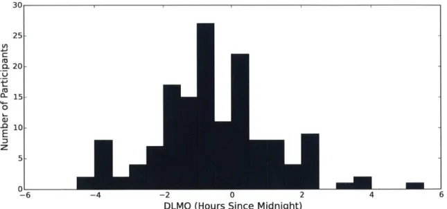
During the course of the 30-day study, each participant was invited to participate in one overnight stay at the hospital. While at the hospital, participants gave saliva samples every hour and completed a test to measure their alertness. From these tests, we were able to compute Dim Light Melatonin Onset (DLMO) for each participant (see Figure 2.7).

4 22 30 25 4-J a 20 15 0 -0 10-E z 5-0 -6 -4 -2 0 2 4 6

DLMO (Hours Since Midnight)

Figure 2.7: Distribution of Dim-Light Melatonin Onset (DLMO) in hours since midnight. For example, 8 participants had a DLMO at 8pm (-4 hours since midnight) and 9 partici-pants had a DLMO at 2am (2 hours since midnight)

2.2.4

Phone Monitoring App

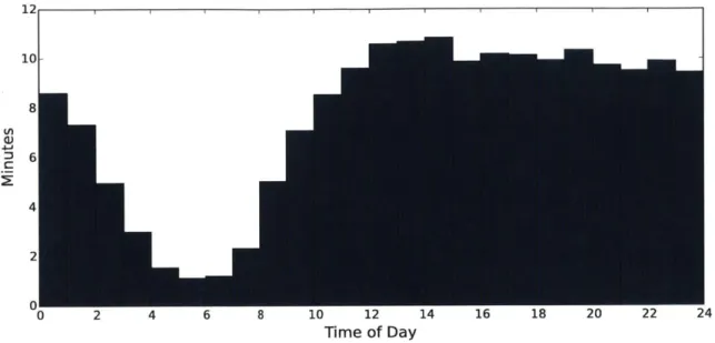
At the beginning of the study, participants downloaded onto their Android Phones a phone monitoring app that collected data, encrypted it, and sent it to our secure servers. This was done passively throughout the study. The app was developed by Akane Sano and was based on the Funf frameworkf 171. It collected, metadata from SMS and calls including the timestamp, the to/from phone numbers, and the duration of calls. Additionally, the app also collected location data (including location source), app usage data, and screen on/off timing (see Figure 2.8 for distribution of the average time spent with the screen on for each hour of the day).

2.2.5

Wearables

During the 30-day study, participants also wore two wearable sensors: the Actiwatch and Affectiva Q-sensor. Participants were instructed to wear these sensors at all times, except when they might get wet (e.g., during showering or swimming).

12 10 8 a) Z) 6 4 2 0 2 4 6 8 10 12 14 16 18 20 22 24 Time of Day

Figure 2.8: Average number of minutes the phone screen was on for each hour of the day

Actiwatch

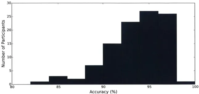
The Actiwatch was worn on the non-dominant hand and recorded light intensity levels and acceleration data. These data were aggregated to one-minute sample rates on the wearable itself and, using proprietary software, automatically determined sleep and wake episodes on the scale of 1 minute. These binary labels were then compared to the self-reported sleeping episodes (see Section 2.2.2) by an expert in order to determine when the participants were

actually sleeping. We found that participants were, on average, 93.5% accurate in reporting sleep episodes (see Figure 2.9). This means that the average participant reported a different sleep/wake state for approximately 28 hours during the study than the expert determined

using the Actiwatch data.

Though there are many measures of sleep regularity, we computed each participant's sleep regularity score based on the expert-labeled sleep/wake episodes on a scale from

0-100 based on the consistency of sleep/wake patterns on a 24-hour period (with sleep

regularity score of 100 being perfectly regular, e.g., same bedtime and wake time each day). In order to compute the sleep regularity score with a period of 24 hours, we let s(t) be the indicator function with s (i) = 1 during wake and s(1) = -1 during sleep, T = 24

hours and T =total number of hours of data, then

I1

Figure 2.9: Distribution of how accurate participants were in self-reporting sleeping episodes compared to the expert label

This score was defined and computed by the Brigham and Women's Hospital (BWH) Team of the SNAPSHOT study and has been used in several of their publicationsl4, 11, 12]. The distribution of sleep regularity scores for our population is given in Figure 2.10.

40 5U btU. /U

Sleep Regularity Figure 2.10: Distribution

sleep regularity score was

bu

of Sleep-Regularity Scores. See the Equation computed

90 100

2.1 for how the 25[ L 0 -Q E z 20-15 10-5 40 35 : (U 0 E z 30- 25- 20- 15- 101-5 30

Q-Sensor

The Q-Sensor was worn on the dominant hand and recorded electrodermal activity (EDA), skin temperature, and 3-axis accelerometer data, at a sample rate of 8Hz. An example of a

9 hour period of data from the Q-Sensor is given in Figure 2.1 1. We focus on electrodermal

activity signals for much of the remaining chapters of this thesis.

6-

43

-2 3 4 5 6 7 8 9 10 11

Time of Day (a) Electrodermial Activity 35.0 34.5 34.0- 33.5- 33.0- 32.5- 32.0-31.5 31.0 30.51 2 3 4 5 6 7 8 9 10 11 Time of Day (b) Temperature 4.0 3.5 3.0 2.5 -0) 2.0 -2 3 4 5 6 8 9 10 11 Time of Day (c) Acceleration

Figure 2.11: Example of Q-Sensor Data from one participant over a 9 hour period (from 2am to I I am). We note that the participant was sleeping from 2am to 7:40am which can easily be seen in the acceleration data

Chapter 3

Electrodermal Activity Data

3.1

Background

Electrodermal activity (EDA) refers to the electrical activity measured on and under the sur-face of the skin [7]. EDA has frequently been used in studies related to affective phenomena and stress because EDA tends to increase as the body responds to arousal or exertion (e.g., [20, 21, 26, 27, 34, 36, 44]). In addition, increases in EDA have also been observed during sleep when arousal and exertion are typically low. In particular, it has been shown that if "sleep storms" (the pattern of many successive EDA responses during sleep) are present they usually occur during slow-wave sleep [25, 28].

In general, electrodermal activity analysis splits the signal into tonic and phasic sig-nals. Tonic signals refer to the slow-moving level of electrodermal activity, whereas phasic signals, also called electrodermal responses (EDRs)', are short in duration and have a char-acteristic shape. Boucsein provides a description of the charchar-acteristic shape of an EDR: the response typically lasts between 1-5 seconds2, has a steep onset and an exponential decay, and reaches an amplitude of at least 0.01pS (see Fig. 3.1 for an example of a typical EDR) [7]. These responses were originally studied in research labs and were observed after a stimulus was presented to the study participant. However, EDRs have also been observed when no stimulus appeared to be present; these are often called spontaneous EDRs.

In the following sections, we will discuss different methods of detecting EDRs and the 'There are several different methods of measuring electrodermal activity, including measuring skin con-ductance. If skin conductance is measured, electrodermal responses are also called skin conductance re-sponses (SCRs).

2

While a single EDR typically lasts 1-5 seconds, EDRs can overlap; that is, another EDR can begin before the first has finished.

28 4.34 4.32 - 4.30-4.28 4.26 4.24 4.22 0 1 2 3 4 5 6 seconds

Figure 3. 1: A typical EDR selected from a SNAPSHOT participant's data. We can see that this EDR lasts about 5 seconds, and it has the typical steep onset and exponential decay.

different features that can be computed from them. We note that because we have collection trillions of data points over the course of the study, we needed an efficient method to process the data. We used Tributary, an interactive distributed analytics platform for large-scale time series data Il l, to simply and efficiently process the EDA data.

3.2

Electrodermal Response (EDR) Event Detection

There exist several methods for identifying EDR events in EDA data. One of the most popular methods is the Ledalab package for MATLAB 15, 61. This package uses

convolu-tion methods to identify EDRs by assuming that the shape of the EDRs for a single person remains the same across time. A newer method called cvxEDA uses convex optimization to split the data into phasic, tonic, and noise components to identify EDR events 118]. This method also assumes that the shape of the EDRs is stable for the same person. While both of these methods have their merits, we have noticed that the EDR structure may change for a person, thus violating the assumptions of both techniques. Furthermore, both methods appear to have been designed for laboratory settings, while we are interested in ambulatory observations where a more diverse experience may elicit different EDRs.

Therefore, we use a simple peak detection algorithm in order to find EDRs. In particu-lar, we identify the apex of the EDR as a peak in the EDA data (after it has been low-pass filtered with an FIR-filter with 64 taps and I Hz cutoff) that has a derivative of at least

0.064pS/.s within 0.5 seconds prior to the identified apex (see Figure 3.2). We note that

were used by Sano et. al. 138, 371, and 0.093/S/s was used by Healey [19]3). This method tends to over-estimate the number of peaks identified compared to Ledalab and cvxEDA methods, but we have created an artifact detection algorithm to reduce the number of false positives (see Chapter 4 for more details).

5.3 - EDA 5.2 Detected EDR 5.1-5.0 4.9 4.8- 4.7- 4.6-4.5 0 10 20 30 40 50 60 seconds

Figure 3.2: Example of identified EDRs (apex identified by vertical red lines) detected using our peak detection algorithm on a SNAPSHOT participant's data. Less abrupt peaks at approximately 5 and 50 seconds are not included with this particular set of parameters.

3.3

Electrodermal Response Features

Once an EDR has been detected, we can compute several features about the basic shape as suggested by Boucsein 171: apex value, rise time, decay time, width, amplitude, and maximum derivative. In order to compute these features, we also need to compute the start and end times of the EDR. Boucsein suggests that the start of the EDR is when the derivative drops below I % of its maximum value and the end time to be defined as the time when the signal drops to less than 50% of the amplitude of the EDR. The width of the EDR is defined as the time delta between when the signal reaches 50% of the amplitude during the rising phase to when the signal falls below 50% of the amplitude on the decaying side. 3_{A1 of these thresholds were originally chosen to conform with the theory of EDRs and were found to be}

appropriate based on visual inspection; however, future research into better detection algorithms that don't assume a single EDR response is needed. For example, a multi-threshold approach might work well.

0

30

Figure 3.3 displays the shape features on an EDR and Table 3.1 gives the computed values of the example EDR.

5.1 - EDA Amplitude - RiseTime 5.0 Width AUC 4.9 4.8 4.7 0 12 3 4 5 6 seconds

Figure 3.3: After a peak has been detected, we can compute a number of features, includ-ing amplitude, rise time, width, and AUC (approximated by multiplyinclud-ing the width by the amplitude [71). See the text for details on computation and Table 3.1 for computed values.

Table 3. 1: Computed EDR Feature Values

Feature Name Apex Value Rise Time Width Amplitude AUC

Value 5.055 1S 2.125 , 2.375 s 0.385 /6 0.915 /S.

Additionally, we can plot histograms of these shape parameters to see how the shape of EDRs for one person can vary within and between sleep and wake (see Figure 3.4). In particular, we note that the apex value and rise times of identified EDRs during sleep were much larger than those identified during wake for this participant on a single day.

In addition to features computed on a single EDR, researchers are often interested in the frequency or rate at which these responses appear. Because these responses appear with irregular patterns, Fourier analysis has not been found to be useful. Generally, simple features (e.g., the number of events in a time window) are computed in order to approximate the rate of EDR events. However, these simple methods of feature extraction are lacking in the ability to capture both the historical effects (when an EDR is detected in the recent history, how does that effect the current probability of an EDR event) and the time-of-day or day-in-sequence effects. We will discuss a better way to capture rate features in Chapter 5.

10 0 LU 0 E 0 - Sleep EDRs LI]Wake E[)R' 0 0 05 L-00 05 10 5 20 25 30 35 40 seconds

(a) Apex Value (b) Rise Time

120, 0 LUJ 0 2 Ln LU1 E z 100 80i 40 20 U'-0 1 2 J 1 6 seconds (c) Width - Sleep EDRs 00 [I Wake EDRs 50 00 200 -150 0 LU) 0 100 -z 10 15 2.0 2.5 30 (d) Amplitude 250 - Sleep EDRs [1] Wa4e EDRs a: LU 0 z 4 6 8 10 12

(e) Maximum Derivative (f) AUC

Figure 3.4: Each subfigure shows a different EDR feature during sleep (blue) and wake (red) for one day's worth of data for a single SNAPSHOT Participant. There were 456 EDRs identified during 5 hours and 40 minutes of sleep and 558 EDRs identified during 16 hours and 20 minutes of wake.

- Sleep EDRs [ Wake EDRs LA LU 0 E z 70 60 50 40 30 20 10 0 'IS Sleep EDRs [IE Wake EDRs

I

III

Chapter 4

Artifact Detection

4.1 Introduction

As discussed in Chapter 3, electrodermal activity (EDA) has been used in several studies in order to relate affective phenomena and stress (e.g., [20, 21, 26, 27, 34, 36, 44]). As these studies have moved from the laboratory environment to ambulatory studies, there is a much greater need to detect artifacts, or noise, in the EDA signal. Electrodermal artifacts typically arise from movement of the skin or muscles beneath the electrodes or pressure changes causing a change in the surface area of the skin in contact with the electrodes [7]. These artifacts are especially likely during ambulatory studies with wrist-worn sensors (like SNAPSHOT) where the participant is going about his or her normal activities which may include walking, riding in a vehicle, typing on a keyboard, or writing.

The most typical way to remove artifacts is by low-pass filtering the EDA signal or using exponential smoothing [21, 27, 33, 36]. This technique is able to remove small noise variations, but is unable to handle the large increases or decreases in EDA signal that often occur when the pressure on the electrodes changes. Others have used heuristic techniques to identify artifacts by looking for abnormal signal variations (e.g., very rapid increases or decreases, or small EDR widths) [20, 27, 41]; however, these techniques only have established thresholds for particular studies, and were only verified through visual inspection. Therefore, these heuristic measures are not guaranteed to generalized to other settings. Others have suggested only considering data during which there is no movement (as determined by an accelerometer). This method, however, cannot detect artifacts due to pressure changes or skin-to-electrode contact changes. The final, least sophisticated way of identifying artifacts requires an expert to look through the signal and manually identify

34

portions of the signal containing artifacts.

Because we have collected over one-hundred thousand hours of EDA data, having an expert label all the data is not feasible. Furthermore, we want to be able to know which por-tions of our signal contain artifacts without having to rely on heuristic techniques. There-fore, we have created a simple machine learning algorithm to identify which 5-second portions of and EDA signal contain artifacts. We have published two papers on this topic and they are reproduced in their entirety in Appendix A and B. In the following sections, we will give the high-level overview of each paper.

4.2 Automatic Identification of Artifacts in Electrodermal

Activity Data

In our first paper published at the IEEE Engineering in Medicine and Biology Conference in 20151, we were able to train a simple binary classifier to identify artifacts in five-second portions of EDA data and achieved 95.7% accuracy on a hold-out test set.

We had two experts label 1,301 5-second portions of EDA signal as containing an ar-tifact or clean based on a common criteria2_{. We then considered two types of classifiers:} binary and multiclass. The binary classifier only used portions of the signal that the ex-perts agreed on, whereas the multiclass classifier included a third class (which we named "questionable"). We then extracted several features from the EDA signal for each 5-second period related to the EDA signal's shape. The data were then split into 3 data sets: training, validation, and testing. Using Wrapper feature selection, a subset of features was chosen using a training set. After trying several different machine learning methods, support vector machines (SVMs) were chosen to be the best and a sweep of SVM parameters was con-ducted in order to choose the best SVM model using training and validation sets. Finally, the selected models (one for the binary classifier and one for the multiclass) were tested on the held-out test set to produce the final results.

Furthermore, in order to achieve this result and allow the model to be able to be easily used by other researchers, we developed an online tool that helps labeling portions of up-loaded data, identifying EDRs, and automatically detecting artifacts. This tool is called

EDA-Explorer and can be found at http: //eda-explorer.media.mit.edu/.

This tool allows a group of researchers to join as a team. The team can then upload files in

'The full paper is reproduced in Appendix A

2

several different formats in order to automatically label artifacts or detect peaks using the online system. We also realized that while our criteria for artifacts would work for similar ambulatory studies, they might not work for other studies like seizure detection where large increases in the EDA signal should be treated as a part of the signal instead of noise. Ad-ditionally, we realized that there is great value in being able to have a system for manually labeling EDA data. For these reasons, we also created the ability for teams to manually label their own data. Teams can require a certain number of labels for each 5-second epoch and track their labeling progress.

We have also open-sourced our code for researchers that would like to use our classi-fiers and EDR detection code offline in batch mode. This code is available at

https://github.com/MITMediaLabAffectiveComputing/eda-explorer/.

4.3 Active Learning for Electrodermal Activity

Classifica-tion

In our second paper published at the IEEE Signal Processing in Medicine and Biology Symposium (SPMB) in 2015', we wanted to expand on our first paper and reduce the human labeling effort by using active learning techniques. We were able to reduce labeling effort by as much as 84% in our applications. This was accomplished by using a variety of SVM-based active learning techniques that intelligently ask the human for labels on 5-second periods.

In comparing the active learning techniques, we used the same dataset as the paper discussed in Section 4.2 and a new data set of EDRs where each 5-second period was labeled as containing an EDR or not. We found that the Simple Margin technique [10] performed very well on both data sets. Furthermore, when we used the automatic stopping criterion associated with the Simple Margin technique, the active learner stopped requesting new labels after about 100 samples in the artifacts data set and after about 150 samples in the EDR data set (1/6th and 1/5th the number of samples required by the passive learner, respectively). Furthermore, even though the active learner required fewer labels than the passive learner, very similar held-out test accuracies were achieved.

3

Chapter

5

Point Process Modeling

5.1

Background

While much work has been done in the lab to figure out why and when electrodermal re-sponses (EDR) happen, less is known about these rere-sponses in ambulatory monitoring es-pecially during sleep. Spontaneous electrodermal responses during sleep, or sleep storms, have been observed since the 1960s (e.g.,[25, 28, 29]). Although counter-intuitive to an emotional arousal interpretation, these studies have found that sleep storms occurred most frequently during slow wave sleep and least frequently during REM sleep. However, all of these studies were conducted in sleep lab environments and for a limited number of nights. Recently, Sano et. al. has conducted a series of studies monitoring EDA while partic-ipants slept at home or in a sleep lab for an extended period of time [37]. In addition to duplicating the results of high probabilities of sleep storms during slow-wave sleep, Sano et. al. provide several characteristics of typical EDA patterns during sleep at home, in-cluding typical numbers of EDR events detected over the night and in 30s time windows. However, this study fails to capture the more complicated dynamics of these sleep storms both within a night and across several days. Furthermore, the rate of electrodermal re-sponses is typically captured in features like the total number of rere-sponses in a window of time; however, we are suggesting that this does not fully capture the information present in the signal because it does not have a dependence on the historical rate of EDRs.

In the computational neuroscience field, recent developments in the state-space point process' have allowed researchers to study between-trial and within-trial neural spiking dynamics [16]. The state-space point process model was developed because other models

38

of systems with time-varying parameters (like the Kalman Filter) are not well suited to the problem of impulse trains because of their assumptions about the data. Since its original development, the state-space point process model has been used to model several different kinds of neuronal data (e.g., [13, 39, 43]) and heart rate data (e.g., [2, 3]). Furthermore, the state-space point process was developed to provide a framework for statistical inference. We use the state-space generalized linear model (SS-GLM) introduced by Czanner et. al. to model electrodermal responses during sleep [13]. This model was chosen for its ability to capture between-night and within-night dynamics of a point process.

In Section 5.2, we provide high-level details about how the model is defined and how models are selected from a group of candidate models. Section 5.3 discusses the proce-dure we used for individually fitting and selecting models for SNAPSHOT participants, including a discussion on why we chose to model EDR events during sleep. We present our results in Section 5.4.

5.2

State-Space Generalized Linear Model

A detailed description of the State-Space Generalized Linear Model is given in the Czanner et. al. paper [13]. We give only the high-level details in this section and provide derivations in Appendix C.

State-space models have been used for many years in many fields including engineer-ing, statistics, and computer science and are sometimes called hidden Markov or latent process models. They are made up of two governing equations: the observation equation and the state equation. The observation equation models how observed events are related to the state. In this case we will use a point process that depends on both within a single night (within-night) and between multiple nights (between-night) dynamics to model our observations (i.e., a series of EDRs across several successive nights). The state equation defines an unobservable process switching between states; this equation will represent the between-night dynamics of EDRs. In the case of EDR event modeling, the state will refer to the level of EDR event detection during a time window.

5.2.1

Observation Equation

We model our data (a series of EDRs across several nights) as a point process: a time-series of random binary

{0,

by a conditional intensity function [13]. For this model, we define a conditional intensity function at time t given the history of EDR events (Ht) up to time t as A(tIHt). Given an EDR event train of duration T, we define N(t) to be the number of EDR events counted in an interval (0, t] for t E (0, T]. Thus, the conditional intensity function is defined as:

A(t IH) i. Pr [N(t + A) - N(t) =11Ht (5.1)

We see that the probability of a single-spike in a small interval (t, t + A] is approximately A (t

I

To simplify the model, the CIF can be defined for discrete time by choosing the number of subintervals, L, to split the observation window. That is, we divide the time interval T into L subintervals of width A = TL- 1. We choose L large enough so that the subinterval contains at most I event. These subintervals are indexed by 1 for I

C

we are interested in modeling how this event train evolves across several nights, we index

the nights by k (where k C {1, ... , K} with K being the total number of nights).

Let nk,l be equal to 1 when there is an EDR event in the interval ((I - 1)A, lA] on

night k and 0 otherwise. Finally, let Hk,I be the history of events in night k, up to time lA. This allows us to write a conditional intensity function for the EDR event train recorded at time lA of night k as the product of the time since sleep onset component, AS(lAI 1), and history component, AH(lA|K, Hkj), as follows:

Ak(lAIOk, _y, Hk,) = AS(IA Ok)AH(lAjy, Hk,I) (5.2)

where 0

k determines the effect the time since sleep onset has on the EDR event activity (i.e., they define the between-night dynamics) and -y determines how the probability of an EDR event at the current time depends on the recent history of EDR events.

In particular, we model the effect of the time since sleep onset (in units of EDR events per second) on EDR events by assuming the following form for the stimulus component:

R

log AS(lAIok) Z Ok,,g,(lA) (5.3)

r=1

where g,(IA) is one of R functions that models the time since sleep onset effect. The choice of g, (1A) functions is flexible, and could be polynomials, splines, or unit pulse func-tions. We choose to use non-overlapping unit pulse functions in order to follow Czanner et. al. [13]. Additionally, this will provide the ability to compare directly with traditional peristimulus time histogram (PSTH) models that are very similar to the way researchers

40

typically approximate EDR event rates.

The g, (lA) functions are parameterized by 0

k [k,1, . ..ak,R] for each night k; thus there is a different 0_{k for each night k. This allows us to model how the time into the night}

effects the EDR event rate during different nights. The relationship of the 0_{k parameters is}

governed by a state-space equation which we describe in Section 5.2.2.

Following Czanner et. al., we model the history component of the conditional intensity function (see Eqn. 5.2) at time lA as a function of history parameters -y and the EDR event history Hk, as a dimensionless component. The history component takes on the following form:

log AH(lA 1y, Hk,l) = I yjnfk,l-j (5.4) j=1

where -y =[71, ... , ,-Y] and nrk, is a binary indicator of whether an event happened at time lA

in trial k. We note that because Eqn. 5.4 only requires J time-steps into the past, we only

need to save those J binary indicators in the history variable Hk,= {=fnk,I-J, ... , nk,I-1}.

Also, we note that the EDR event parameter -y is independent of night, k. Thus, this compo-nent of the conditional intensity function seeks to model the underlying biophysical prop-erties of EDR events.

Putting Eqn. 5.2, 5.3, and 5.4 together, the conditional intensity function (or observation equation) becomes:

R

A(lA10k, O , HkI) = exp E,,g,(1A) exp yjnkl-j (5.5)

r=1 j=1

5.2.2

State Equation

Now that we have described the observation equation (see Eqn. 5.5, we now define the state equation as a simple random walk model following Czanner et. al. [13]. In particular, we define the equation as:

Ok = Ok-1 + Ek (5.6)

where Ck is an R dimensional Gaussian random vector with mean 0 and unknown covari-ance matrix E. This covaricovari-ance matrix will be estimated using Estimation Maximization techniques described below. We note that smaller values of E will give smaller average differences between stimulus components of successive nights (Ok-1 and Ok).

5.2.3

Estimation of Model Parameters using Expectation

Maximiza-tion

Now that we have both an observation equation (Eqn. 5.5) and a state equation (Eqn. 5.6), we need a method to estimate the unknown parameter ) = (-, 0o, E). As pointed out by Czanner et. al., because Ok is unobservable and V) is unknown, we use the Expectation Maximization (EM) algorithm to compute their estimates. The derivation of this algorithm for our set up of this model is given in Appendix C.

This algorithm gives us the parameter estimates of 0

kjK and

4'

Z)-5.2.4

Goodness-of-Fit

Because standard distance measures are not suitable for point-process data, we use the time re-scaling theorem to transform the point-process EDR event data into a continuous measure so that we can apply appropriate goodness-of-fit tests[8, 32]. The re-scaled times, Zk,m are computed for each EDR event m in each night k as follows:

Zk,m 1 - CX - ,m-1 kK, ,

Hk,u)du

where Uk,m is the time of EDR event m. in night k. If the conditional intensity function is a good approximation to the true conditional intensity of the point process, the re-scaled times Zk,m, will be independent, uniformly distributed random variables on the interval [0, 1). We note that because Eqn. 5.7 is one-to-one, we can directly compare the rescaled times to a uniform distribution to assess the goodness-of-fit of the model.

First, we evaluate whether the Zk,,n are uniformly distributed by ordering them from smallest to largest and denoting the ordered values as zm where rn* = 1, ..., M with M being the total number of observed spikes. We then plot these ordered re-scaled times zm*

against the quantiles of the cumulative distribution function of the uniform distribution on [0, 1). We note that the quantiles are defined as bm, = (m* - 0.5)/M. Czanner et. al. term this plot as a Kolmogorov-Smirnov (KS) plot and note that if the model is consistent with the data, then the points should lie on the 450 line. We note that the Kolmogorov-Smirnov statistic for our model is the supremum of the (vertical) distances between the K-S plot and the 45' line. Thus, smaller K-S statistics indicate a better model fit.

Next, we evaluate whether the Zk,r, are independent by taking advantage of the struc-ture of the model and assessing the independence of the Gaussian transformed re-scaled

42

times (zkm) by analyzing their autocorrelation structure. In particular, we transform Zk,r using the cumulative distribution function of a standard Gaussian random variable, <D(.), as follows:

G

Zkm = D(Zk,m) (5.8)

We can then determine the degree to which the Gaussian transformed re-scaled times, zm are independent by plotting their autocorrelation function (ACF). We can then count the number of ACF values that are outside a 95% confidence interval around zero to

approxi-mate the independence of the re-scaled times up to lag 100. We note that smaller numbers of ACF values outside this confidence interval indicates a better model fit.

5.2.5

Model Selection

Because there are several hyper-parameters that can be set (e.g., number of lagged history parameters J and the number of unit impulse functions R), we can fit several models to the EDR event data. We use Akaike's Information Criterion (AIC) to identify the best model [9]. The AIC score is a combination of the log likelihood of the model and is penalized for higher numbers of parameters; it is computed as follow:

AIC(p) = -2 log P(N\V) + 2p (5.9)

where p is the number of parameters of the model and log P(N IV) is the log likelihood of the observed data. Thus, in theory the model with the smallest AIC score is the best model; however, following Czanner et. al., we acknowledge that small fluctuations in AIC scores appear. Therefore, if two models have AIC scores within 10, we choose the model with fewer parameters.

5.2.6

Special Cases of the State-Space Generalized Linear Model

In the simplest case, we could assume that effect of the time since sleep onset is the same for all nights and that there is no dependence on EDR event history; that is, we could assume that 0

k = {Ok,1, ..., Ok,R} = 0 = {1, ... OR} for all k and A H(lA Hk,i) = 1 for

R

Ak(IAO) = exp E rgr(lA) (5.10)

T--1

Note that the conditional intensity function, Ak(lAJO), is the same for all nights k.

Furthermore, since we have chosen the functions g,(iA) to be non-overlapping, equal width unit pulse functions, this model has become an inhomogeneous Poisson Process and is equivalent to a peristimulus time histogram (PSTH). The 0 parameters can be easily estimated by counting the number of EDR events that occurred during the time determined

by the unit pulse functions. In particular, 0, is the number of EDR events that occurred

between times 1A = [(r - 1)LR-1 -I+ 1]A and iA = [rLR1 ]A summed across all nights.

It is worth noting that this PSTH model is what is commonly used in EDR event mod-eling currently; that is, typical EDR event modmod-eling estimates the rate of EDR events using only counts of these events without considering how the rate might be effected due to recent EDR events or what happened during a previous night.

The other special case of the SS-GLM allows there to be a history dependence to the EDR event rate, but still assumes that the effect of time since sleep onset is the same for all nights (Wk - {0k,1, ..., 0k,R} = 0 = {1, ... , OR} for all k). Thus, the conditional intensity

function for this model has the form:

RJ

Ak(IAK-, 0, Hk,l) = exp

{

{

r=1 j=1

Thus, unlike the PSTH model, this model has a different conditional intensity during dif-ferent nights because it depends on the EDR event history of that night. It can therefore capture between-night dynamics, but only those due to different EDR event trains. We refer to this model as the Static Generalized Linear Model (Static-GLM) with a log-link, and it can be solved using fitting procedures in various out-of-the-box solvers.

5.3

Modeling EDR events during sleep

After collecting 1000s of hours of electrodermal activity data from 164 participants over the course of 30 days of home-sleep during the SNAPSHOT study (see Chapter 2 for more details), we then used our binary artifact detection algorithm described in Chapter 4 to detect artifacts for all collected data. Thus, every 5-second period of electrodermal activity data was labeled as containing artifacts or containing no artifacts (see Figure 5.1 and 5.2 for

I

examples). We observe that many more artifacts are detected during wake periods which makes sense because individuals are moving and adjusting their wearable sensor (the most common causes of EDA artifacts) more while awake.

3.2 30 2.8 2.6 24 2.2 2,0 1.8 16 14 0 5 10 15 minutes 20 25 30

Figure 5. 1: Detected electrodermal activity artifacts have been labeled in red. This data set comes from a SNAPSHOT participant during sleep. The noise in this example is most likely due to the participant moving during sleep and the pressure on the Q-sensor changing resulting in a different skin conductance measurement.

20 1,8 1.6 14 1.2 - 1.0 0.8 0.6 04 02 0 5 10 15 minutes 20 30

Figure 5.2: Detected electrodermal activity artifacts have been labeled in red. This data set comes from a SNAPSHOT participant during wake. Here the noise is likely due to the participant walking around or moving his or her wrist while talking, writing, or working on a computer.

In addition to observing more artifact-free data during sleep, we hypothesized that EDR events would be more consistent in timing from night-to-night given the previous literature on EDA during sleep. For these reasons, we decided to continue our analysis looking at EDR events during sleep only. We used a combination of self-reported sleep time cross-validated by an expert with access to the participant's actigraphy data from the Actiwatch in order to determine when the participant was asleep (see Chapter 2 for more information). Using the EDR event detection method described in Section 3.2, we detected EDR events for each night (see Figure 5.3 for an example of one participant's detected EDR

A.J

IW