Condition Monitoring Using Automatic Spectral Analysis

HAL Id: hal-00084894

https://hal.archives-ouvertes.fr/hal-00084894

Submitted on 10 Jul 2006

HAL is a multi-disciplinary open access archive for the deposit and dissemination of sci-entific research documents, whether they are pub-lished or not. The documents may come from teaching and research institutions in France or abroad, or from public or private research centers.

L’archive ouverte pluridisciplinaire HAL, est destinée au dépôt et à la diffusion de documents scientifiques de niveau recherche, publiés ou non, émanant des établissements d’enseignement et de recherche français ou étrangers, des laboratoires publics ou privés.

Condition Monitoring Using Automatic Spectral

Analysis

Corinne Mailhes, Nadine Martin, Kheira Sahli, Gérard Lejeune

To cite this version:

Corinne Mailhes, Nadine Martin, Kheira Sahli, Gérard Lejeune. Condition Monitoring Using Au-tomatic Spectral Analysis. Structural Health Monitoring, Jul 2006, Granada, Spain. pp.1316-1323. �hal-00084894�

Cover page

Title: Condition Monitoring Using Automatic Spectral Analysis Authors: Corinne Mailhes

Nadine Martin Kheira Sahli Gérard Lejeune

Corinne MAILHES, IRIT - TéSA - ENSEEIHT, 2 rue Camichel, BP7122, 31071 Toulouse Cedex 7, France, [email protected]

NadineMARTIN, Kheira SAHLI, Gérard LEJEUNE, LIS - BP 46, 961 rue de la Houille Blanche, 38402 Saint Martin d'Hères Cedex, France, [email protected]

ABSTRACT

Within the frame of machinery maintenance, spectral analysis is a helpful tool. Therefore, an automatic spectral analysis tool, capable to identify each component of a measured signal would be of interest. This paper studies a new spectral analysis strategy for detecting, characterizing and classifying all spectral components of an unknown process. Indeed, any vibration signal can be considered as a mixture of components, a component being either a sinusoidal wave, or a narrow band one. We assume that a sum of an unknown number of these components is embedded in an unknown colored noise. The complete methodology we propose provides a way to feature each component in the spectral domain.

The first idea is not to choose one specific spectral analysis method but, rather, to concatenate the results of complementary algorithms. For each one, the noise spectrum is estimated by a nonlinear filter and spectral component detection is managed with a local Bayesian hypothesis testing. This test is defined in frequency and takes account of the noise spectrum estimator. Thanks to a matching with the corresponding spectral window, each component detected is classified into one of the following four classes: Pure Frequency, Narrow Band, Alarm and Noise.

The second main idea is then to propose a fusion of the classification results, leading to a complete description of each spectral component present in the signal. This spectral classification is particularly interesting within the context of condition monitoring. Examples are given on real vibratory signals and show the performance of the proposed automatic method, which is particularly well adapted to signals having a high number of components.

INTRODUCTION

Machine condition monitoring is of great interest for machinery maintenance as faults should be detected before they become serious. Vibration analysis is popular as a predictive maintenance procedure and as a support for machinery maintenance decisions. In spite of a huge research in spectral analysis, there is always a real need for an automatic spectral analysis tool, capable to identify each component of a measured signal.

This paper studies a new spectral analysis strategy for detecting, characterizing and classifying spectral structures of an unknown stationary process. A spectral structure is defined as a sinusoidal wave called Pure Frequency (PF), a Narrow Band signal (NB) or a Noise peak (N). A sum of an unknown number of these structures is embedded in an unknown colored noise. Spectral analysis of such signals is interesting in several applications, including vibratory, acoustic, seismologic or radar signal processing. In these application fields, signals are rich in spectral components and therefore, windowed discrete Fourier Transform remains a useful tool even if the problem can after that be formulated in a more specific application framework.

The strategy proposed is automatic and based on the use of complementary spectral analyses. An optimal method does not always exist and it seems to us to be of interest to take all the properties of diverse analyses into account. Few approaches have been actually published in this context. The spectral analysis developed in [1] is automatic but focused on the estimation of the period length of one periodic signal by minimizing a cost function in frequency. In [2], the authors define a local least square approach in the frequency domain, the signal being modeled by a sum of sinusoids and a white noise. More recently, the authors in [3] came up with the idea of using two different bandwidth resolutions but with two signal measurements, not always available.

In this paper, we propose to match up a number of L spectral analysis methods. Within the framework of investigated signals, we focus on Fourier based methods, the choice being the result of a trade off between low variance, high frequency resolution and low window leakage properties [4]. These L methods provide L estimates of the Power Spectral Density (PSD) γ νˆ_i

( )

, i=1,…,L of the signal through, what we called,

L cycles. The methodology proposed provides a way to calculate the identity card of

each peak, similarly to a real I.D. card. Indeed, this I.D. card results from the fusion of L intermediate cards, calculated at each cycle, and permits the classification of each peak into the right class, PF, NB or N as mentioned above. Note that we have already published some part of this work in [4], [5]. After recalling the interpretation cycle and the classification in a nutshell, this paper aims at demonstrating the interest of such an automatic analyser in the field of vibration analysis.

INTERPRETATION CYCLE

The interpretation cycle is a two-step procedure. First, signal peaks are detected through a multi-PFA scheme. Second, a spectral adjustment with the spectral window of the estimator is applied to each peak detected, leading to the creation of the intermediate cards describing the spectral structure.

Multi-PFA detection

The first step of the interpretation cycle consists of making decisions about two possible statements; a peak of the PSD γ ν_i

( )

corresponds to noise (H0 hypothesis) or

to signal (H1 hypothesis). At each frequency ν, this problem can be formulated as a

hypothesis test where

( )

( )

( )

( )

( )

0 :γ νi =γ νb 1 :γ νi =γ νs γ νb

with γ ν_b

( )

the continuous PSD of a zero mean stationary Gaussian noise and γ ν_s

( )

( )

2

a PSD of a stationary random process or a deterministic signal belonging to L R . Since the distribution of γ νˆ_i

( )

under H1 is not easy to find, the optimal test statistics cannot be found. However, we propose a test statistics of the following form

( )

( )

0 1 ˆ γ ν µ γ ν ≤ = > % H i b H T , (2)

with γ ν_%b

( )

an estimation of the noise PSD γ ν_b

( )

estimated by filtering γ νˆ_i

( )

. After having compared median, percentiles, morphologic and 2-pass mean filters [4], we propose an original iterative method combining detection steps and a nonlinear n-pass mean filter [4], [6]. Based on this, we are able to derive the distribution of the proposed test statistics (2) in the case of hypothesis H0. The distribution of T is a F-distribution [10] and the decision threshold µ in (2) can be adjusted from a given Probability of False Alarm (PFA).

Since the probability of non-detection under H1 is not easy to compute, we propose a multi-PFA test rather than fixing only one value of PFA. A set of PFA values is chosen. At each detected peak referred to as γˆ_{p i,}

( )

ν , p=1,…,Pi, (Pi being the peak number of γ νˆ_i

( )

), we assign the lowest PFA, which has allowed detection. This PFA, called joint PFA, gives an indication about the local noise level of the peak.

Spectral adjustment

The second step of the interpretation cycle is classification of peaks detected in the first step. We propose an iterative adjustment between each peak and the spectral window related to the spectral estimator of cycle i. This window, denoted by Q_{p i,}

( )

ν , is oversampled and centred on each peak γˆ_{p i,}

( )

ν such that the normalized quadratic error defined as

( )

( )

(

)

(

)

2 1 2 , , 2 , max ˆ ( , ) ˆ γ ν ν γ ν = − =

∑

k p i k p i k k k _{p i k} Q e p i ,p=1,...,P , (3) _i

is minimized given that _max =arg max

(

γˆ_{p i,}

( )

ν_k

)

k

k .Values k1 and k2 are determined depending how the error is calculated, either from all of the points on the peak main lobe, or from points above the -3 dB level only. These quadratic errors are therefore denoted etot(p,i) and e-3dB(p,i) respectively. Contrary to a maximum likelihood approach, this method is suboptimal but incurs a rather low computational expense, which is a necessary requisite owing to a possible large number of peaks. Signals of interest can have hundred of components, see for example spectrum of signals in communication [7], in biomedical [8] or in vibratory mechanics [9].

Thanks to Monte Carlo (MC) simulations described in [5], the spectral structures investigated are identified as regions in the error space (etot(p,i), e-3dB(p,i)). We then

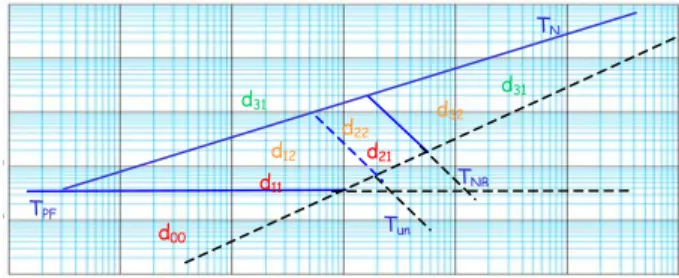
define a distance, which can be considered as a measure of membership degree of a peak towards a specific region or class. So as to, at each region delimited by the thresholds shown in Figure 1, we associate an integer distance dkl where index k, ranged between 0 and 3, identifies the region, and index l a spectral pattern: l=0 for PF, l=1 for an uncertainty between PF and N, and l=2 for NB.

Tun TNB TN TPF d00 d31 d12 d31 d21 d22 d32 d11

Figure 1 - Class contours defined from Monte Carlo simulations and parameterized by dkl. Class

PF=d00; class NB=d32, class Noise=d31. Others regions are uncertainty classes.

Class PF, characterized by the minimal distance d00,is located at low errors under the straight line TPF=0, defined as a line up to the PF cluster got at SNR equal to 0 dB in MC simulations. Afterwards, the more the errors increase, the more the peak departs from a PF. At the opposite, class N, characterized by the higher distance d31,is located at the highest errors above another straight line TN=0 defined as the line up to the PF and NB clusters got at SNR equal to -20 dB in MC simulations. Intermediate distances, d11 and d12, measure an uncertainty between PF and N peaks, delimited by the line Tun, and such as

00 = <0 11 < 21< 31

d d d d . (4)

Class NB, characterized by a mean distance d32, is located under TN but above a third line TNB, defined, in the same way, as the line down the NB cluster got at SNR equal to 0 dB. The narrower the NB, the closer to the PF cluster. Thus, an increasingly weak distance is associated to these regions delimited by the same line Tun such as

00 = <0 12 < 22 < 32

d d d d , (5)

Tun, is defined as the separation between PF and NB clusters at SNR equal to –15 dB. In the central region where TN≤0 and TPF>0, an uncertainty between PF

below TNB, or N above TNB, at low SNR and NB at high SNR is removed with the

joint PFA. A joint PFA equal to 10-5 or 10-6 will detect NB peaks.

Finally, at each couple (k,l) is given a numerical value such as dkl=kd1l, with a given initial value d1l. This classification can be locally extended to multi-component signals embedded in a correlated Gaussian noise. At last, for each γˆ_{p i,}

( )

ν , a set of characteristics can be given: the adjusted central frequency, the time amplitude, the mean noise variance, the local SNR, the emerging SNR which depends upon the estimator (see Section Application), the adjustment errors, the frequency interval

I(CiPp) or a peak frequency base defined as the –3dB bandwidth, the joint PFA

referred to as PFAi and the distance (dkl)i. This list is referred to as an intermediate card of the peak.

CARD FUSION AND CLASSIFICATION

Intermediate cards are established for each γˆ_{p i,}

( )

ν and for each cycle, i=1,L. A null card, with a distance higher than the value associated to noise, is added when a peak is not detected at one cycle. So as to associate cards corresponding to the same peak, a simple criterion is defined

I(CiPp) I(CjPp')∩ ≠ ∅, i≠ j , (6)

with I(CiPp) being the frequency interval defined above. The connected cards form a set called a sequence. Owing to its construction, a sequence describes the same spectral structure, which is also represented by L points in the error space.

In each sequence, the intermediate cards are merged according to the following procedure. If the sequence presents more than one uncertainty (non constant index l in

dkl over the sequence), if alarms on PFA (two far PFA are not accepted) or on the noise level were set on, the peak is classified into an Alarm class, which points out a bad estimate of the noise spectrum. Afterwards, in each sequence, distances are combined as

( )

( )

2 ₂ 1 1 1 _σ 1 = = =

∑

L =

∑

L

peak kl i peak kl peak

i i

d d and d d

L L i − . (7)

The final distance d_{peak f,} is defined as

, =min_, ,

peak f _{k l} peak kl

d d d , (8)

and determines the final spectral pattern of the peak. The standard deviation σpeak allows the computation of a stability index Stpeak, which indicates the stability of the results on the sequence with a known maximum standard deviation σ_max,

(

max

)

100 1 σ σ

= −

peak peak

St . (9)

A final PFA, PFApeak, is calculated as

(

)

1 1 = =

∏

L L peak i i PFA PFA . (10)

The final card is called the spectral I.D. and gathers these new characteristics. The final distance dpeak is used to classify all the peaks in one of the following classes: PF, NB, N and Alarm. Finally, it is important to notice that the detection probability of a peak is high if the classification yields a high stability index and a low final

PFApeak simultaneously.

peak St

APPLICATION TO VIBRATION ANALYSIS

A test was performed on an experimental platform in order to identify vibrations induced by the hydraulic noise of an oil station. Several devices such as a soft water pump and motors were operating on the platform. The data analysed in this section (see figure 2) were acquired by an accelerometer located close to the oil station of

which we want to determine the vibration signature. The sampling frequency is 3 KHz and the anti-aliasing filter has a cut-off frequency equal to 1,25 KHz. The stationarity of the measure has been checked by applying the time-frequency detector described in [11]. The spectrum depicted in figure 2 also indicates the presence of a significant number of modes and of a non-white noise. The methodology presented in this paper is applied and we will discuss the results within the frequency range 0-100Hz only.

Figure 2. Hydraulic noise in time (left) and in frequency (right)

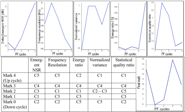
Main objective being PF detection, no frequency average is introduced and L is set at 5: an hybrid periodogram-correlogram with Blackman window (cycle 1), a Welch-Wosa first with Blackman window (cycle 2) then with Hanning window (cycle 3), a Blackman-Tuckey first with Blackman window (cycle 4) then with Hanning window (cycle 5) [4]. Performance of the chosen methods are depicted in figure 3.

Emerg-ent NSR

Frequency

Resolution Energy ratio Normalizedvariance quality ratioStatistical Mark 4 (Up cycle) C5 C5 C2 C1 C1 Mark 3 C4 C4 C4 C4 C4 Mark 2 C3 C1 C1 C2 – C3 C5 Mark 1 C1 C3 C3 - C3 Mark 0 (Down cycle) C2 C2 C5 C5 C2

Figure 3 – Values of 5 criteria characterizing spectral analysis performance (up) and assessment of a mark at each cycle (down) of the PF strategy and for data presented in figure 2.

The first criterion is referred to as the Delta Emergent Noise to Signal Ratio (NSR). The emergent NSR indicates how the method makes the peak more emerged in frequency. A low equivalent bandwidth of the spectral window as in cycle 5 leads to a high added value of 12.2 dB. Cycle 2 has the minimum adding value equal to 9.8 dB. The other criteria are classical one in spectral analysis: the frequency resolution deduced from the –3dB bandwidth of the spectral window, the normalized variance,

the percentage of energy ratio characterizing the spectral leakage and the statistical quality ratio defined by the product of the normalized variance and the normalized statistical bandwidth of the spectral window [4]. The assessment of a mark as derived in figure 3 reveals drawbacks and advantages of each cycle.

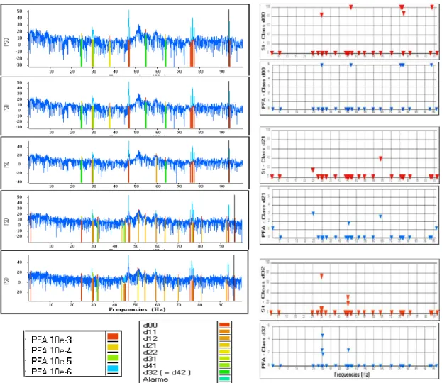
Figure 4 summarizes the results of the detection and classification proposed in this paper. Left hand side of figure 4 presents spectra get from the 5 cycles mentioned above. The colored up peaks correspond to the peaks detected by test (2). As can be seen, the different estimated PSDs do not lead to the same detected peak set, reinforcing the idea of using jointly all these different analyses. Right hand side of figure 3 displays the results of 3 classes according to the stability index (9) and the final PFA (10) for the 38 peaks detected. The other classes have not been represented since they are all empty, except for the Alarm and N classes.

Figure 4. On the left, zoom spectra of the hydraulic noise within the frequency range 0-100Hz for L cycles with L=5. Peaks detected are colored according to distance dkl (below the noise line) and to PFA

(above the line spectrum). On the right, results of the classification proposed according to both the stability index (St) and the final PFA (exponent of the value) for class PF (d00), uncertain class between

PF and N (d21) and class NB (d32).

The final distance d00 has been assigned to 6 peaks at frequencies 29.8 Hz, 46.9 Hz, 75.8 Hz, 76.6 Hz, 77.3Hz and 93.74 Hz with stability indexes greater than 80%. These peaks having the lowest final PFAs (equal to 10-6) are PF without doubt. We are less confident with the two peaks detected in class d21 at frequencies 24.8 Hz and

62.9 Hz because of lowest stability index and final PFA. By the same way, the peak at 30.1 Hz with a distance d32 belongs to class NB but with even less confident, 73 % only, whereas the four other ones, at frequencies 32.4 Hz, 32.6 Hz, 45.2 Hz et 45.3 Hz, have a too high final PFA and a too low stability index to be considered. The other peaks, 38 were detected over the frequency range studied, belong to class N or to the Alarm class. The analysis of the complete frequency band, not presented in this paper, conclude to the occurrence of two families of harmonics, one with a fundamental at 46.9 Hz and another one at 76,6 Hz. This last one has two lateral bands with an harmonicity of 0.8 Hz. The methodology proposed focused on the detection of PF and NB embedded in an unknown non-white noise. So the wide band structure at frequency 51.4 Hz is not and cannot be detected. Future works are in progress for adding this class in the system.

CONCLUSION

The strategy of spectral analysis presented in this paper leads to an automatic process for detecting, characterizing and classifying sinusoidal waves and narrow band signals of an unknown stationary process. This kind of tool is of interest for fault detection and machinery maintenance. The idea of fusion of different spectral analysis methods is original in signal analysis field. Operating spectral estimator properties allows a rigorous and accurate identification of spectral peaks, which breaks free from a visual interpretation.

REFERENCES

1. J. Schoukens, Y. Rolain, G. Simon, R. Pintelon, Fully automated spectral analysis of periodic signals, IEEE Tr. Ins. Meas., Vol 52, n°4, August 2003, pp.1021-1024.

2. L-M. Zhu, H-X. Li, H. Ding, Estimation of multi-frequency signal parameters by frequency domain non-linear least squares, Mech. Syst. and Sig. Proc., Elsevier, Vol. 19, 2005, pp. 955-973. 3. D. Rabijns, G. Vandersteen, W. Van Moer, An automatic detection scheme for periodic signals

based on spectrum analyzer measurements, IEEE Trans Instr. Measur., vol 53, n°3, June 2004. 4. M. Durnerin, Une stratégie pour l’interprétation en analyse spectrale, détection et caractérisation

des composantes d’un spectre, INPG PhD thesis, September 1999, www.lis.inpg.fr.

5. N. Martin, C. Mailhes, K. Sahli, G. Lejeune, Vers une Carte d'Identité Spectrale, 20ème colloque GRETSI sur le Traitement du Signal et des Images, Louvain-la-Neuve, Belgique, Sept. 6-9, 2005. 6. W.A. Struzinski, E.D. Lowe, A performance comparison of 4 noise background normalization

schemes proposed for signal detection systems. JASA., n°. 78, Sept. 1985, pp. 936-941.

7. L.O Hoeft, J.L. Knighten, J.T. DiBene II; M.W. Fogg, Spectral analysis of common mode currents on fibre channel cable shields due to skew imbalance of differential signals operating at 1.0625 Gb/s, IEEE Int. Symp. on EC, Vol. 2, 24-28, Aug. 1998.

8. M. Drinnan, J. Allen, P. Langley, A.Murray, Detection of sleep apnoea from frequency analysis of heart rate variability, Computers in Cardiology 2000, 24-27 Sept. 2000, pp. 259-262.

9. N. Martin, P. Jaussaud, F. Combet, Close shocks detection using time-frequency Prony Modelling. MSSP, Mechanical Systems and Signal Processing, Vol. 18, n°2:, March 2004. pp. 235-261. 10. N.L.Johnson, S. Kotz, N. Balakrishnan, Continuous univariate distribution, vol 2, Wiley Edition,

1994.

11. N. Martin, A criterion for detecting nonstationary events, Twelfth International Congress on Sound and Vibration, ICSV12, Lisbon, Portugal, July 11-14, 2005.