Long-term variations of the UV-B radiation over Central Europe as derived from the reconstructed UV time series

HAL Id: hal-00317322

https://hal.archives-ouvertes.fr/hal-00317322

Submitted on 8 Apr 2004

HAL is a multi-disciplinary open access

archive for the deposit and dissemination of

sci-entific research documents, whether they are

pub-lished or not. The documents may come from

teaching and research institutions in France or

abroad, or from public or private research centers.

L’archive ouverte pluridisciplinaire HAL, est

destinée au dépôt et à la diffusion de documents

scientifiques de niveau recherche, publiés ou non,

émanant des établissements d’enseignement et de

recherche français ou étrangers, des laboratoires

publics ou privés.

Europe as derived from the reconstructed UV time series

J. W. Krzyscin, K. Eerme, M. Janouch

To cite this version:

J. W. Krzyscin, K. Eerme, M. Janouch. Long-term variations of the UV-B radiation over Central

Europe as derived from the reconstructed UV time series. Annales Geophysicae, European Geosciences

Union, 2004, 22 (5), pp.1473-1485. �hal-00317322�

Annales Geophysicae (2004) 22: 1473–1485 SRef-ID: 1432-0576/ag/2004-22-1473 © European Geosciences Union 2004

Annales

Geophysicae

Long-term variations of the UV-B radiation over Central Europe as

derived from the reconstructed UV time series

J. W. Krzy´scin1, K. Eerme2, and M. Janouch3

1_{Institute of Geophysics, Polish Academy of Sciences, Warsaw, Poland} 2_{Tartu Observatory, T˜oravere, Tartumaa, Estonia}

3_{Solar and Ozone Observatory, Czech Hydrometeorological Institute, Hradec Kralove, Czech Republic}

Received: 1 October 2003 – Revised: 19 December 2003 – Accepted: 23 January 2004 – Published: 8 April 2004

Abstract. The daily doses of the erythemally weighted UV

radiation are reconstructed for three sites in Central Europe: Belsk-Poland (1966–2001), Hradec Kralove-Czech Repub-lic (1964–2001), and T˜oravere-Estonia (1967–2001) to dis-cuss the UV climatology and the long-term changes of the UV-B radiation since the mid 1960s. Various reconstruc-tion models are examined: a purely statistical model based on the Multivariate Adaptive Regression Splines (MARS) methodology, and a hybrid model combining radiative trans-fer model calculations with empirical estimates of the cloud effects on the UV radiation. Modeled long-term variations of the surface UV doses appear to be in a reasonable agreement with the observed ones. A simple quality control procedure is proposed to check the homogeneity of the biometer and pyra-nometer data. The models are verified using the results of UV observations carried out at Belsk since 1976. MARS pro-vides the best estimates of the UV doses, giving a mean dif-ference between the modeled and observed monthly means equal to 0.6±2.5%. The basic findings are: similar climato-logical forcing by clouds for all considered stations (∼30% reduction in the surface UV), long-term variations in UV monthly doses having the same temporal pattern for all sta-tions with extreme low monthly values (∼5% below overall mean level) at the end of the 1970s and extreme high monthly values (∼5% above overall mean level) in the mid 1990s, re-gional peculiarities in the cloud long-term forcing sometimes leading to extended periods with elevated UV doses, recent stabilization of the ozone induced UV long-term changes be-ing a response to a trendless tendency of total ozone since the mid 1990s. In the case of the slowdown of the total ozone trend over Northern Hemisphere mid-latitudes it seems that clouds will appear as the most important modulator of the UV radiation both in long- and short-time scales over next decades.

Key words. Atmospheric composition and structure

(biospheric-atmosphere interaction) – Meteorology and atmospheric dynamics (climatology; radiative processes)

Correspondence to: J. W. Kryz´scin

(jkrzys@igf.edu.pl)

1 Introduction

The ultraviolet (UV) radiation reaching the ground is only a small portion of the radiation received from the Sun but extremely important for the Earth’s ecosystem. Increased in-terest in the variations of the surface level of the UV radia-tion, that has appeared since the late 1980s stemmed from the anticipated positive UV trend over the extratropical regions related to the observed total ozone decline (e.g. Madronich, 1992). The changes in the global UV field are of special im-portance because of the recognized wide adverse effects of excessive UV radiation on humans and the environment (e.g. sunburn, snow blindness, skin cancer, cataracts, suppression of immune system, etc.).

Since the early 1990s, available resources have been ap-plied to improve our knowledge of the UV changes and our understanding of processes that affect surface UV radiation. Research efforts in the area of the atmospheric physics have placed a large emphasis on the calibration and maintenance of the existing UV observing systems, the development of new instruments and QA/QC methods, and the data analy-ses using the results from both ground-based and satellite UV instruments (WMO, 2003). There was limited interest in the UV radiation measurements before the period of the large total ozone decline. Thus, the time series of the sur-face UV-B measurements longer than 2 decades are avail-able for only one station in Europe-Belsk. The length of reliable data records is up to 10–15 years for most Euro-pean UV observing stations. It is recognised that such a pe-riod is not adequate to carry out trend analyses (Weatherhead et al., 1998). However, in some recent studies the ground-based/satellite measurements and model simulations have been used to identify changes in the surface UV and pro-cesses responsible for the UV radiation changes (e.g. Kerr and McElroy, 1993, Borderwijk et al., 1995; Zerefos et al., 1995; Krzy´scin, 1996; Weatherhead et al., 1997; Udelhofen et al., 1999; den Outer et al., 2000; Kaurola et al., 2000; Matthijsen et al., 2000; Eerme et al., 2002). These studies confirm that the UV changes are driven by various factors: ozone, cloudiness, aerosols, and surface albedo. The relative importance of these factors depends on local conditions.

Studies on the impact of UV radiation on the environ-ment require knowledge of UV climatology and changes that have occurred in the past. Recently, various models using variables directly affecting the UV radiation (total ozone, cloud/aerosol optical depth) and proxies parameterizing the UV transmittance through the atmosphere (total solar radia-tion, sunshine duraradia-tion, and cloud cover) have been used to reconstruct surface UV radiation (e.g. Ito et al., 1993; den Outer et al., 2000; Fioletov et al., 2001; de La Casini`ere et al., 2002). The pyranometer and other meteorological data serve as proxies for the combined cloud/aerosols effects on UV radiation. The reconstructed data sets, which can extend backward in time to the beginning of total ozone and pyra-nometer or cloud observations, would help to examine the climatology and the long-term variations and trends of UV radiation (Kaurola et al., 2000; Fioletov et al., 2001).

In this study we examine several UV reconstruction mod-els to estimate the UV long-term pattern and to delineate factors influencing its variations for selected sites in Central Europe–Hradec Kralove (50.1◦N, 15.5◦E), Belsk (51.7◦N, 20.8◦E), and Tartu/T˜oravere (58.3◦N, 26.5◦E). Section 2 de-scribes the data used with special emphasis on the quality assurance of the UV data and its proxies. Section 3 deals with the model descriptions and comparisons. We exam-ine two categories of the reconstruction models, i.e. a purely statistical model based on the Multivariate Adaptive Regres-sion Splines (MARS) methodology and a model combining radiative transfer calculations for clear-sky conditions with the empirically derived cloud reduction factor of the UV ra-diation derived from the attenuation of total solar rara-diation. The factors responsible for the UV long-term variations and the regional differences in the UV forcing are discussed in Sect. 4. Section 5 contains the conclusions.

2 The data used

The idea of the reconstruction is to reproduce the surface UV variations using variables that may parameterize the attenu-ation of the UV radiattenu-ation passing through the atmosphere. It is well recognized that the following variables are indis-pensable to describe the UV attenuation: total ozone, air mass (solar zenith angle-SZA), aerosols and cloud micro-physical (e.g. single scattering albedo, and asymmetry fac-tor) and macrophysical properties (e.g. optical depth). We need a long-term series of these variables (3–4 decades) and a reconstruction model to discuss the UV climatology and trends. The validation of the reconstructed time series should be accomplished by a comparison with the UV observations over the model/measurements, with the common time peri-ods being as long as possible.

The total ozone observations have been carried out over many places in the Northern Hemisphere mid-latitudes since the late 50s and early 60s. The results of the ozone mea-surements were stored in a global data base (World Ozone Data Center-WODC) at Toronto, Canada. The long-period WODC ozone data underwent a careful homogenization

pro-cedure and was used in many statistical analyses (e.g. Bo-jkov et al., 1995; WMO, 2003). Here we use the ozone data from the Dobson spectrophotometer measurements at Hradec Kralove (1964–2001), Belsk (1966–2001), and the filter ozonometer M-124 and Dobson measurements at St. Petersburg (1973–2001), the nearest station to T˜oravere pro-viding the total ozone data. The total ozone time series for Hradec Kralove and Belsk are longer but the length of the an-alyzed series was limited by the onset of the ancillary data.

There are no continuous measurements of the cloud and aerosols properties which are important for the determination of the UV attenuation through the atmosphere besides short-period campaigns. However, the combined cloud/aerosols affects on the surface UV radiation can be parameterized us-ing the so-called clearness index, Clear I nd Gl, i.e. the ra-tio of measured total solar irradiance (or its daily sum) to the hypothetical (derived from radiative transfer calculations) value of the total solar irradiance that would occur under the same conditions but without clouds (e.g. Janouch, 2000; Kaurola et al., 2000). Thus, the clearness index provides a measure of the cloud effects on the total solar radiation. Since we are dealing with the long-term series of the clear-ness index, the question of the homogeneity of this series im-mediately arises. Total solar radiation measurements belong to standard observations carried out at many meteorological stations including those examined here. However, such long-period measurements were made using various pyranome-ters (e.g. Kipp@Zonnen Moll-Gorczynski solarigraph, CM5, CM6, CM11, and Sonntag PRM2 in the case of observations at Belsk since the mid 1960s) and now it is difficult to re-calculate the historical time series accounting for all instru-mental and calibration changes to obtain the homogenized data set. Here we propose a simple quality control procedure to check the long-term homogeneity of the total solar and UV-B radiation measurements. Later in the paper we will concentrate on the surface radiation measured mostly during the warm part of the year (April–September) due to the high intensity of the radiation in that period contributing signifi-cantly to the annual mean of the radiation. It is also possible to calculate the clear-sky UV daily dose without detailed in-formation on the surface conditions that is required for the late autumn/winter/early spring time because of the highly variable snow cover over Central Europe.

The clear-sky values of daily irradiance for all days with the measured daily sum of total solar radiations have been estimated by the Santa Barbara DISORT Atmospheric Ra-diative Transfer (SBDART) code (Ricchiazzi et al., 1998). The calculation for the chosen SZA requires a selection of various input parameters, among them the most impor-tant ones, changing significantly from one day to another, are aerosol optical depth (AOD) and columnar water vapor content. Other variables as vertical profiles of temperature and trace gases were kept equal to climatological means de-pending on season and region, e.g. mid-latitudinal summer or winter. The daily changes of the columnar water vapour amount were taken from the NCEP/NOAA Reanalysis-2 data base (presently available at this Web address: http://nomad2.

J. W. Krzy´scin et al.: Long-term variations of the UV-B radiation over Central Europe 1475

24

Figure 1. The differences between measured and modelled daily sums of total solar radiation

in percent of the modelled values for clear-sky conditions during the period April-September

for Belsk (1966-2001) - (a), Hradec Kralove (1964-2001) - (b), and Tõravere (1967-2001) -

(c). The differences between measured and modelled daily doses in percent of the modelled

values for clear-sky conditions over Belsk (1976-2001) - (d). The solid curves represent the

differences after a smoothing by LOWESS technique

1 9 6 4 1 9 6 8 1 9 7 2 1 9 7 6 1 9 8 0 1 9 8 4 1 9 8 8 1 9 9 2 1 9 9 6 2 0 0 0 Y e a r - 2 0 - 1 5 - 1 0 - 5 0 5 1 0 1 5 2 0 2 5 - 2 0 - 1 5 - 1 0 - 5 0 5 1 0 1 5 2 0 2 5 ( c ) T o r a v e r e ( % ) 1 9 6 4 1 9 6 8 1 9 7 2 1 9 7 6 1 9 8 0 1 9 8 4 1 9 8 8 1 9 9 2 1 9 9 6 2 0 0 0 Y e a r - 2 0 - 1 5 - 1 0 - 5 0 5 1 0 1 5 2 0 2 5 - 2 0 - 1 5 - 1 0 - 5 0 5 1 0 1 5 2 0 2 5 ( d ) B e l s k ( % ) 1 9 6 4 1 9 6 8 1 9 7 2 1 9 7 6 1 9 8 0 1 9 8 4 1 9 8 8 1 9 9 2 1 9 9 6 2 0 0 0 Y e a r - 2 0 - 1 5 - 1 0 - 5 0 5 1 0 1 5 2 0 2 5 - 2 0 - 1 5 - 1 0 - 5 0 5 1 0 1 5 2 0 2 5 H r a d e c K r a l o v e ( b ) ( % ) 1 9 6 4 1 9 6 8 1 9 7 2 1 9 7 6 1 9 8 0 1 9 8 4 1 9 8 8 1 9 9 2 1 9 9 6 2 0 0 0 Y e a r - 2 0 - 1 5 - 1 0 - 5 0 5 1 0 1 5 2 0 2 5 - 2 0 - 1 5 - 1 0 - 5 0 5 1 0 1 5 2 0 2 5 B e l s k ( a ) ( % )

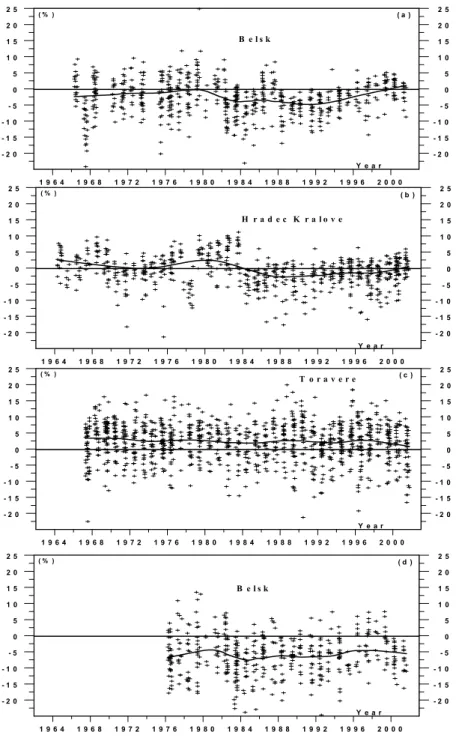
Fig. 1. The differences between measured and modelled daily sums of total solar radiation in percent of the modelled values for clear-sky conditions during the period April–September for Belsk (1966–2001) (a), Hradec Kralove (1964–2001) (b), and T˜oravere (1967–2001) (c). The differences between measured and modelled daily doses in percent of the modelled values for clear-sky conditions over Belsk (1976-2001) (d). The solid curves represent the differences after a smoothing by the LOWESS technique.

ncep.noaa.gov/ncep data) comprising the global distribution, with a resolution of 2.5◦×2.5◦, of various meteorological variables. The long-term variations of AOD over selected sites were not available. Thus, we use constant values of AOD at 550 nm (equal to 0.25) and the ˚Angstr¨om exponent (equal to 1.3) in the model calculations of total solar irra-diance. Both values result from averaging all CIMEL Sun photometric measurements of spectral optical depth carried out over the AERONET network in Central Europe in

re-cent years (Belsk, T˜oravere, and Potsdam). The data were taken from the AERONET web page presently at address http://aeronet.gsfc.nasa.gov.

Sunshine duration (from measurements by the Campbell-Stokes heliograph) data let us determine cloud free days. Moreover, these data are also tested as one of the regres-sors in the pure statistical model (MARS). Figure 1 shows the time series of the differences between the observed and modeled daily sum of total solar irradiances (in percent of the

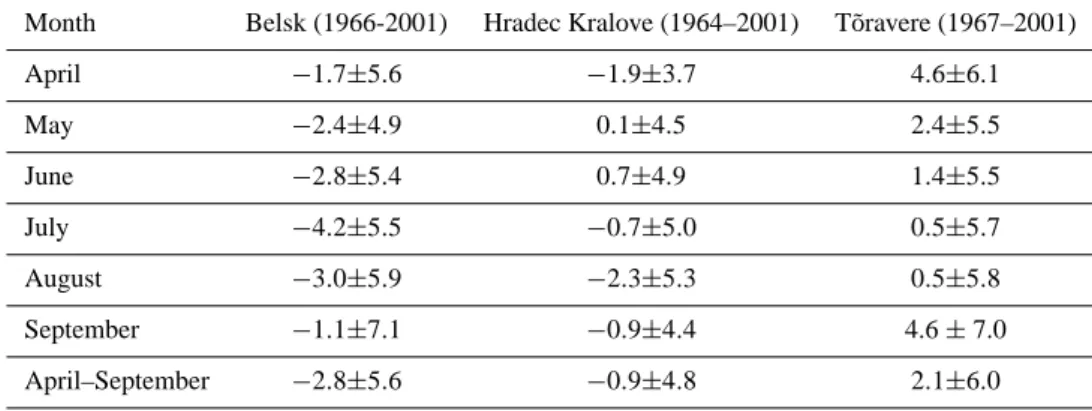
Table 1. The differences between the observed and modeled daily sum of total solar radiation for clear-sky conditions (in percent of clear-sky values) for selected months and the April–September period.

Month Belsk (1966-2001) Hradec Kralove (1964–2001) T˜oravere (1967–2001) April −1.7±5.6 −1.9±3.7 4.6±6.1 May −2.4±4.9 0.1±4.5 2.4±5.5 June −2.8±5.4 0.7±4.9 1.4±5.5 July −4.2±5.5 −0.7±5.0 0.5±5.7 August −3.0±5.9 −2.3±5.3 0.5±5.8 September −1.1±7.1 −0.9±4.4 4.6 ± 7.0 April–September −2.8±5.6 −0.9±4.8 2.1±6.0

modeled value), i.e. the so-called fractional deviations, for approximately cloudless days during April-September peri-ods, i.e. for days when a bias between the measured sunshine duration and the modeled one for clear-sky conditions was less than 0.5 h. The modeled sunshine duration was calcu-lated as the length of the period with an irradiance exceeding 120 W/m2, i.e. the heliograph threshold for burning a paper.

Large scatter seen in Fig. 1 may be the result of the inac-curacy of the daily measurements of total solar irradiance, of the inability to determine the precise number of cloud free days (presence of thin clouds giving the instantaneous total irradiance above the threshold limit of the heliograph), and of a lack of proper model input (especially for days when aerosol optical properties were much different than the as-sumed constant climatological means). However, the stan-dard deviation of the normalized observation-model differ-ences for all stations is only about 5%. The results of sta-tistical analysis of the differences are shown in Table 1 for each calendar month (April-September) and for the whole season. It seems that the standard deviation of the differ-ences is not very different between the analyzed stations and months. The model for Hradec Kralove provides the small-est value of the standard deviation of the differences. The expected uncertainty of the measured daily sum of total so-lar radiation was estimated (by the producer) to be ±3% for CM11 and ±5–10% for older versions of pyranometers. To detect a long-term pattern of the model-observation depar-tures Locally Weighted Scatterplot Smoothing (LOWESS, Cleveland, 1979) has been applied. A smoothed pattern of the differences shows long-term variations in the range ≤5% of the clear-sky norm.

The time series of the smoothed differences may also pro-vide a scale of the clearness index contamination by instru-mental changes or (if we trust the long-term stability of the measurements) the effect of an incorrect selection of the ra-diative model input (especially AOD), which was kept con-stant in the radiative transfer model simulations. These lead us to the examination of two categories of the data, non-corrected one (we keep daily sums of total solar radiance

as they were) and corrected one (the measured all-sky daily sums are multiplied by a correction function to eliminate the long-term variations of the index delineated from the clear-sky subset of the index). If we assume that the smoothed pat-tern in Figure 1 reflects some instrumental/calibration prob-lems in the past, the proposed correction function is

Cor Gl(t )=1 − (Clear I nd Gl_SMOOTH(t )

−Clear I nd GlMEAN) (1)

where Clear Ind GlSMOOTH(t )is a value of the smooth

func-tion fitted to the daily values of the index, Clear Ind GlMEAN

is an overall mean of the index, and t denotes day since the time series beginning. Solid lines in Fig. 1 show (Clear Ind GlSMOOTH(t)-1)*100 values.

Time series of surface UV-B irradiance are rather short, usually not longer than 1 decade. As far as it is known to the authors, one of the longer time series, which underwent a quality control procedure, comes from Belsk (Borkowski, 2000). Thus, comparison of the Belsk’s time series and the reconstructed series by various models may provide a kind of validation of the models. The measurements of broad-band UV-B irradiance have been carried out at Belsk by means of the Robertson-Berger (RB) instrument in the period 1976– 1992, and the Solar Light (SL) UV-Biometer 501A since 1991. These are broad-band sensors for monitoring bio-logically active radiation. The instruments’ spectral charac-teristics were designed to mimic the spectral sensitivity of Caucasian skin to sunburn (i.e. the erythemal action spec-trum). Calibration of the Belsk RB instrument and a ho-mogenization of the Belsk UV-B time series were discussed by Krzy´scin (1996) and Borkowski (2000). The analyzed daily UV time series comprises the homogenized RB time series for the period 1976–1992, and daily doses from 5-min scans by Solar Light UV biometer (model 501a) since Jan-uary 1993. The estimated uncertainty (by the producer) of daily dose by the biometer is ∼±5%.

The time drift of sensitivity of our UV instruments needs to be examined. It is accomplished in a similar way as for

J. W. Krzy´scin et al.: Long-term variations of the UV-B radiation over Central Europe 1477 total solar radiation, i.e. we extract the smooth pattern of the

clearness index from daily UV doses for cloudless conditions over the whole period of observations. Erythemaly weighted UV-B irradiances at the ground level for clear-sky conditions were calculated using SBDART, taking into account the to-tal ozone values (from the concurrent Dobson spectropho-tometer measurements) and climatological values of AOD at 320 nm (equal to 0.34) representative for the whole UV-B range. Jaroslawski et al. (2003) analyzed almost 10 years observations of AOD carried out at Belsk by means of the Brewer spectrophotometer. They found small AOD changes with wavelength in the UV-B range, keeping constant AOD during radiative model simulations over this range.

Figure 1d shows the time series of daily (Clear Ind

UV-1)*100 values calculated for almost clear-sky days during

the April-September periods. We adopt the same procedure for the selection of those days as that used for the clearness index for total solar radiation. It is seen that the modeled values are about 5% larger than the measured ones, probably because of the cosine error of the UV instrument and inac-curate selection of the climatological aerosols characteristics in the radiative model input. It is worth mentioning the small long-term oscillations in the clearness index revealed by the LOWESS smoother applied to the daily doses. This supports the homogeneity of the UV data and its value for the long-term analyses.

To account for possible small instrumental/calibration changes, we recalculated the all-sky UV daily doses by a cor-rection function,

Cor U V (t ) =1 − (Clear I nd U V_SMOOTH(t )

−Clear I nd U VMEAN) , (2)

where Clear Ind UVSMOOTH(t ) is a value of the smooth

function fitted to the daily values of the index, and

Clear Ind UVMEANis an overall mean of the index. We do

not correct small biases between the observed and modeled daily values (seen in Fig. 1d) because further in the paper the long-term variations of the UV radiation will be extracted from the fractional deviations of the monthly doses (i.e. the differences between the monthly doses and their long-term monthly averages in percent of the long-term averages). The bias has no effect on the fractional differences of the ob-served (or reconstructed) doses. Moreover, if we examine the behaviour of the fractional deviations, there is also no need to correct the instrument readings for its imperfect cosine re-sponse (using, for example, the formula derived by Mayer and Seckmeyer et al., 1996), because the cosine corrections will cancel out in the expression for the fractional deviations.

3 Models of the long-term variations in surface UV-B

radiation

Two kinds of models are examined here to mimic all-sky daily doses. The first one is a standard model multiplying the clear-sky daily dose obtained from the radiative model

25

0.00 0.25 0.50 0.75 1.00 1.25

Clearness Index - global radiation

0.00 0.25 0.50 0.75 1.00 1.25 C learn ess In d ex-erythem al U V SZA<41.40 (a) 0.00 0.25 0.50 0.75 1.00 1.25 1.50

Clearness Index - global radiation

0.00 0.25 0.50 0.75 1.00 1.25 1.50 Cl e arnes s In dex - ery themal UV 72.5o_<SZA (b)

Figure 2. The clearness index for UV radiation versus that for total solar radiation for the

noon values of SZA< 41.4

(a) and SZA>72.5

(b). Solid curve represents the cloud reduction

factors (CRF) used in model A (see text).

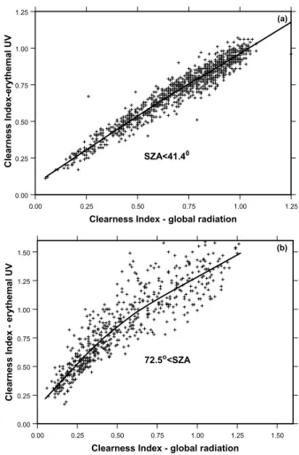
Fig. 2. The clearness index for UV radiation versus that for to-tal solar radiation for the noon values of SZA< 41.4◦ (a) and SZA>72.5◦(b) Solid curve represents the cloud reduction factors (CRF) used in model A (see text).

simulations with the actual value of total ozone and AOD (if possible) by an empirical value of a cloud reduction factor for the UV-B radiation (e.g. Kaurola et al., 2000; den Outer et al., 2000). The second one incorporates an advanced statis-tical technique able to capture both the linear and nonlinear impacts of regressors on the dependant variable, the MARS methodology, initially introduced by Friedman (1991). Mod-els which enable one to calculate daily doses and further sta-tistical analyses will be based on the monthly averages of the daily doses.

3.1 Combined empirical/radiative-transfer model

A model considered here separates the cloud effects on UV radiation from the ozone and aerosols effects as follows,

U Vall−sky, mod(t ) = CRF ∗ U Vclear−sky, mod(t ) , (3)

where UVall−sky,mod(t )and UVclear−sky,mod(t )are model

all-sky and clear-all-sky daily doses for day t , respectively, CRF is the cloud reduction factor depending on the clearness in-dex for total solar radiation. CRF is an estimation of the

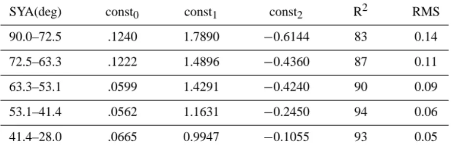
Table 2. Regression coefficients of a second order polynomial fit for the empirical relation of the cloud reduction factors over the UV range (erythemally weighted) versus that of total solar radiation for various SYA ranges. The parameters describing the quality of fit: explained percent of variance- R2, and RMS values.

SYA(deg) const0 const1 const2 R2 RMS

90.0–72.5 .1240 1.7890 −0.6144 83 0.14 72.5–63.3 .1222 1.4896 −0.4360 87 0.11 63.3–53.1 .0599 1.4291 −0.4240 90 0.09 53.1–41.4 .0562 1.1631 −0.2450 94 0.06 41.4–28.0 .0665 0.9947 −0.1055 93 0.05

clearness index for UV radiation obtained from the regres-sion of the clearness index for the daily UV doses on the clearness index for daily sums of total solar irradiance. Both indices came from the concurrent measurements of the UV daily doses and total solar radiation at Belsk for the period 1976–2001 and normalized by the modeled clear-sky values. Clear-sky doses (daily sums of global radiation) are calcu-lated using a radiative transfer model, the SDBDRT model, with observed total ozone (column amount of water vapor from the Reanalyses-2 data base) and constant aerosols char-acteristics.

CRF dependence on SZA and Clear Ind Gl has been

ex-amined for various ranges of the noon values of SZA. We select the same SZA subclasses as those proposed by den Outer et al. (2000). For example, in Fig. 2 we present

Clear Ind UV values versus those of Clear Ind Gl for the

same days for two extreme ranges of noon SZA, i.e. with the lowest and highest noon SZAs, Fig. 2a (SZA<41.40)

and Fig. 2b (SZA>72.50). It is worth noting that the much larger scatter seen in Fig. 2b is due to snow effects (these large SZAs occur in December and the early Jan-uary period at Belsk usually with variable snow cover). The solid lines show a polynomial least-squares fit to the indices data, giving an estimation of Clear I nd U V dependence on

Clear I nd Gl,

CRF =consto+const1Clear I nd Gl

+const2Clear I nd Gl2. (4)

The coefficients of the fit for all considered SZA classes are in Table 2. den Outer et al. (2000) used a power func-tion to estimate the CRF dependence of the clearness index of total solar radiation. Their cloud reduction factor of the erythemally weighted UV-B daily doses was

CRF = A ∗ [1 − (1 − Glall−sky,measured/

Glclear−sky,mod)1/P], (5)

where A and P are regression constants. Further in the text a model using CRF as given by Eqs. (4) and (5) will be denoted as model A and A1, respectively.

It is difficult to decide if the long-term oscillations in the smoothed normalized differences (shown in Fig. 1) reflect the changes in the instrument sensitivity or variations in the input parameter to the clear-sky model (kept constants in the radiative transfer model simulations, i.e. aerosols character-istics and albedo). Thus, we repeat the calculation of the

CRF using two categories of the data:

– non-corrected radiation data comprising observed daily

UV doses and daily sums of total solar radiation.

– corrected radiation data after application correction

function (1) and (2) to the observed daily sums of to-tal irradiance and daily UV doses, respectively;

The first option means that we assume that real variations in model parameters, set constant in the model runs, are respon-sible for the long-term oscillations in the model-observation differences found under clear-sky conditions. Further in the text the result obtained with such data will be denoted as non-corrected ones. The reconstructed UV fractional deviations will be compared with the observed (and non-corrected) UV fractional deviations.

The second option leads us to the assumption that the in-strument sensitivity fluctuated over the analysed period and the long-term characteristics of aerosols and water vapour did not affect the long-term pattern of the fractional differ-ences. Calculation of CRF and comparisons with the re-constructed data will be done assuming that the correction functions let us eliminate instrumental shift or instrument deterioration. Further in the text the result obtained with such data will be denoted as corrected ones.

We are aware that both model input which is too idealized and the instrument drift modulate the behaviour of the differ-ences. Thus, showing results separately for the corrected and non-corrected classes of data will help us to define bound-aries (or range of changes) for the “natural” long-term os-cillations in the reconstructed data and climatological esti-mates.

J. W. Krzy´scin et al.: Long-term variations of the UV-B radiation over Central Europe 1479 3.2 Pure statistical model - MARS

MARS reveals a relationship between the dependent variable (predictand) and the independent ones (regressors). It has been applied in a wide range of disciplines (e.g. de Veaux et al., 1993a; Taliani et al., 1996; and Finizio and Palmieri, 1998; Krzy´scin, 2003). On problems with a reasonably small number of predictors and when order interactions between them is not larger than 3 (i.e. the regression may have the term xi, xi*xj, and xi*xj*xk, where xi denotes i−th

predic-tor), MARS competes very favorably with nonlinear models, such as artificial neural networks (de Veaux et al., 1993b). The authors suggested that MARS could be used instead of neural nets in a wide variety of applications because MARS was always much faster and more interpretable than a neural net and was often more accurate as well.

MARS starts from an assumption that all selected regres-sors affect the predictand in a complex way. Here we use following regressors: daily mean of total ozone, daily sum of total solar radiation (not corrected or corrected by the instru-mental drift), sunshine duration, and noon value of SZA. It seems that the length of the day is also a possible regressor. However, it was excluded from the list of potential regressors because of its linear dependence on the noon SZA for the an-alyzed part of the year. The number of regressors considered by MARS is extended, also taking into account squares of these predictors. We do not need to calculate the clear-sky values of the radiative variables, as for the previous model, and thus many assumptions of the atmosphere structure are eliminated.

MARS goes through a two-stage procedure. Stage I is a fast search that tests all possible regressors’ influence on the dependant variable, resulting in an overfitted model. Stage II refines the model by eliminating unnecessary redundant re-gressors. The final model retains only the important variable that significantly affects the outcome of the model. For an exhaustive description reference should be made to Fried-man (1991) and application in the atmospheric radiation Krzy´scin (2003). The great advantage of MARS is that it performs the selection of regressors, the interaction order be-tween regressors, and the amount of smoothing, all automat-ically. This is accomplished via a penalized residual sum of squares. The user can tune the degree of penalization, which depends on the number of regressors.

The UV daily doses for the April-September part of the year over the 1976–2001 periods, UVall sky(t ), are

approxi-mated setting initially N =8 regressors xi(t )and maximally

two-way interactions (∼ xixj)between regressors, U V (t ) = N X i=1 fa(xi(t )) + N X i,j,j >i fb(xi(t ), xj(t )) + N oise(t )

N oise(t ) = δN oise(t −1) + Random(t ) , (6)

26 1976 1980 1984 1988 1992 1996 2000 Year -20 -15 -10 -5 0 5 10 15 20 25 Frac tional D ev iati ons Measurements Smoothed Measurements Smoothed Data -Model A Smoothed Data -Model B

(a) (%) 1976 1980 1984 1988 1992 1996 2000 Year -20 -15 -10 -5 0 5 10 15 20 25 Frac tional D ev iati ons Measurements Smoothed Measurements Smoothed Data -Model A Smoothed Data -Model B

(b) (%)

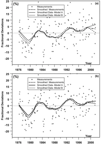
Figure 3. The comparison between the modelled (model A and B) and observed monthly fractional deviations from the UV measurements carried out at Belsk in the April-September part of the year in the period 1976-2001. The measured monthly fractional deviations are superposed on the data smoothed by LOWESS; non-corrected data (a), corrected data (b).

Fig. 3. The comparison between the modelled (model A and B) and observed monthly fractional deviations from the UV measurements carried out at Belsk in the April-September part of the year in the period 1976–2001. The measured monthly fractional deviations are superposed on the data smoothed by LOWESS; non-corrected data

(a), corrected data (b).

where the model residuals, Noise(t), are modeled as first or-der autoregressive process (to account for a part of the UV variations not explained by the regressors used), and func-tions f(...)are a combination of linear left and right truncated

splines (for details, see Krzy´scin, 2003). MARS trimming procedure removes redundant terms of (6), which do not con-tribute remarkably to the quality of the fit. MARS selects the most significant variables affecting the surface UV radi-ation (ordered according to value of the weighted variance explained by the variable) as: global radiation, ozone, and SZA. Further in the text MARS estimates of the fractional UV variations will be denoted as model B results.

3.3 Comparison and verification of the models

The smoothed modeled time series of the monthly frac-tional UV deviations over Belsk during the snowless part of the year for the period 1976–2001 by the combined empirical/radiative-transfer model (model A) and MARS (model B) are shown in Fig. 3, superposed on the monthly fractional deviations derived from the non-corrected (Fig. 3a)

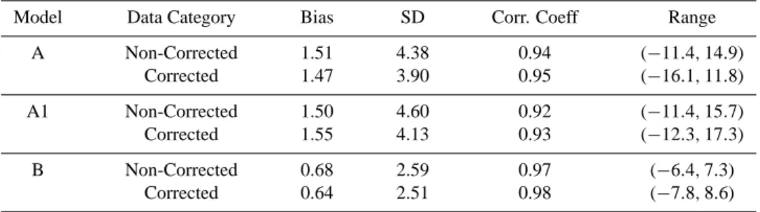
Table 3. The bias, standard deviations (SD), correlation coefficient (Corr.Coeff), and extreme departures (Range) of the differences between modelled and observed monthly fractional deviations by various reconstruction models (in % of the long-term monthly means).

Model Data Category Bias SD Corr. Coeff Range A Non-Corrected 1.51 4.38 0.94 (−11.4, 14.9) Corrected 1.47 3.90 0.95 (−16.1, 11.8) A1 Non-Corrected 1.50 4.60 0.92 (−11.4, 15.7) Corrected 1.55 4.13 0.93 (−12.3, 17.3) B Non-Corrected 0.68 2.59 0.97 (−6.4, 7.3) Corrected 0.64 2.51 0.98 (−7.8, 8.6)

and corrected (Fig. 3b) measured UV daily doses. It is seen that both models quite closely reproduce the long-term vari-ations of the monthly fractional devivari-ations. An apparent in-crease in the UV doses starting at the end of the 70s and lasting throughout the 80s and a kind stabilization since the early 90s can be noted. Models based on non-corrected data are not capable of reproducing an observed light drop in the UV radiation (non-corrected) since about 1998 (Fig. 3a). The modeled UV time series departs only slightly from the ob-served time series over the whole analyzed period after ap-plication of the correction functions (1) and (2). Thus, it sug-gests that probably an instrumental drift could force the drop at the end of the 90s. An alternative way of explaning of the drop is an increase in the aerosols loading in the atmosphere (changes in the aerosol properties were not accounted for by our models). However, recent measurements of the AOD in the UV range over Belsk by the Brewer spectrophotometer in the period 1993–2001 (Jaroslawski et al., 2003) do not sup-port this hypothesis. The same can be also inferred from a smooth pattern of model-observation differences in Fig. 1d. It seems that the behaviour of our biometer at the end of the 90s needs an additional check to identify sources of increas-ing departure between the pattern of smoothed UV variations by model A and that derived from observations.

To compare a performance of each model we calculate the percent of the variance of the original time series that is ex-plained by each model, model-observation bias, the standard deviations of the model-observation differences, maximum positive and minimum negative departure between the mod-eled and observed fractional deviations. Table 3 contains the above mentioned statistical characteristics describing a cor-respondence between the models (A, A1, and B) and obser-vations. Modeled monthly mean doses are always only about 1% greater than the observed values. Use of the corrected data improves only slightly the model-observation agreement (lower standard deviations). All models explain a significant part of the variance of the observed monthly fractional de-viations (>90%). The MARS model provides the best esti-mates of the observed monthly time series (the lowest bias, standard deviation, and the range between the maximum pos-itive and minimum negative departures relative to monthly UV norm, and the highest percentage of explained variance).

The standard deviations of the monthly fractional departures for Belsk (Table 3) correspond to those calculated over the Canadian stations (∼4–5% for summer) by means of regres-sions using total ozone, total solar radiation, snow cover, and dew point temperature (Fioletov et al., 2001). MARS also provides the better estimates of the daily doses, i.e. the overall difference between modeled and observed daily doses in percent of observed daily doses is 0.65±7.88% (1σ ) and 0.65±8.29% for the corrected and non-corrected variables, respectively. Whereas the hybrid models give larger values 1.3±9.1% (model A) and 1.3±10.1% (model A1), both es-timates were derived from the corrected set of variables. It should be mentioned that the MARS simulations of the daily doses are close to the uncertainty (about 5% as given by the producer) of the measured daily doses by the SL biometer-model 501A. Thus, MARS could provide a reasonable esti-mate of the daily doses for days when the UV measurements were not carried out. All models behave similarly when the long-term variations of monthly doses are considered (see Fig. 3).

The UV time series for Hradec Kralove (1996–2001) and T˜oravere (1998–2001) are much shorter than the Belsk’s time series. Thus, in this section the model comparisons have been shown only for the Belsk data. There were not enough data points for other stations to construct a MARS model with so high an accuracy as that for Belsk. If we take MARS re-gressors from observations carried out at Hradec Kralove and T˜oravere and use the Belsk’s MARS constants, such a model will not perform better than the hybrid model. It should be noted that we obtain an almost similar performance of models in the snowless period based on the CRF obtained in various European regions (Belsk-Equation (4), and the Netherlands-Equation (5) given by den Outer et al., 2000). It may suggest that both estimates of the cloud affects on UV as derived from total solar radiation work similarly, so for-mulas are not sensitive to local conditions (opposite to the MARS simulations). Therefore, the reconstructed time se-ries over Central Europe shown in the next section will be obtained using model A and model A1.

J. W. Krzy´scin et al.: Long-term variations of the UV-B radiation over Central Europe 1481

4 UV reconstruction

Using the historical time series of total solar radiation and to-tal ozone we can calculate a hypothetical time series of daily UV doses back to the mid 1960 s. An agreement between reconstructed and observed UV time series during common periods (as discussed in the previous section) builds our con-fidence in the behaviour of the time series for years when UV measurements were not carried out.

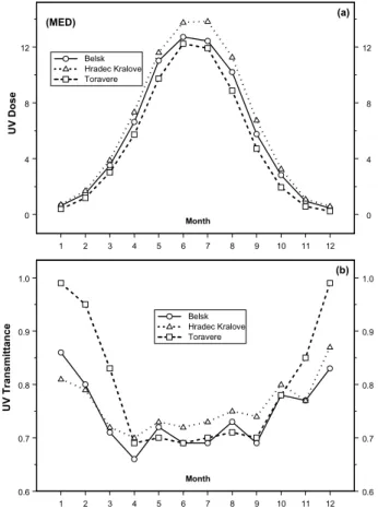
Figure 4 shows long-term monthly characteristics of the surface UV radiation for the common period for all three sta-tions (1967–2001). The seasonal course of the monthly mean UV doses (in Minimum Erythemal Dose–MED unit) is the same (with the spring/summer maximum and winter mini-mum) for all considered stations (Fig. 4a). As is expected the monthly doses decrease with latitude. The maximum dif-ference between the stations (Hradec Kralove and T˜oravere) can be as large as 2 MED (in the snowless period).

Averaging CRF daily values we obtain the seasonal pat-tern of the cloud forcing on the UV-B radiation (Fig. 4b). The attenuation appears quite small in winter because of a high albedo effects (backscattering of the radiation reflected from the surface) that may partially compensate the UV at-tenuation by clouds. The clear-sky norm is calculated as-suming snowless conditions; thus, it is not surprising that the mean UV transmittance might be close to 1 in late au-tumn/winter/early spring season. The snow effects are in-cluded in our model indirectly by calculating CRF for UV radiation based on total solar radiation data and a regression formula for large noon SZA (see Table 2).

The reduction of the UV radiation by clouds is simi-lar over all considered stations (∼30% in the period April-September). During the months when snow cover may ap-pear, the albedo effects can offset the cloud effects, yielding smaller departures of the all-sky daily doses from the the-oretical clear-sky values calculated for snowless conditions. The UV monthly doses for T˜oravere appear close to clear-sky doses in the December–February period. Thus, it means that the snow can increase the surface doses by 20–30%, which agrees with previous estimates of the snow effects on the UV radiation.

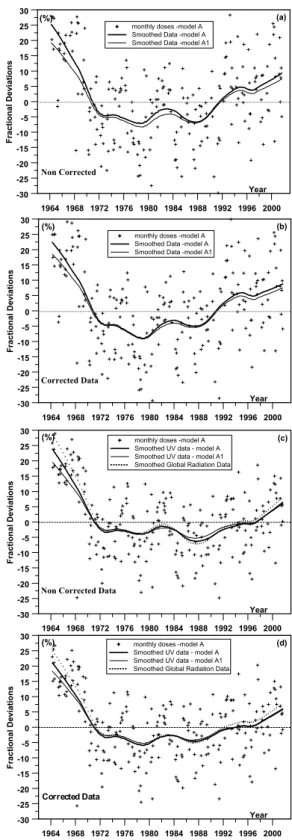
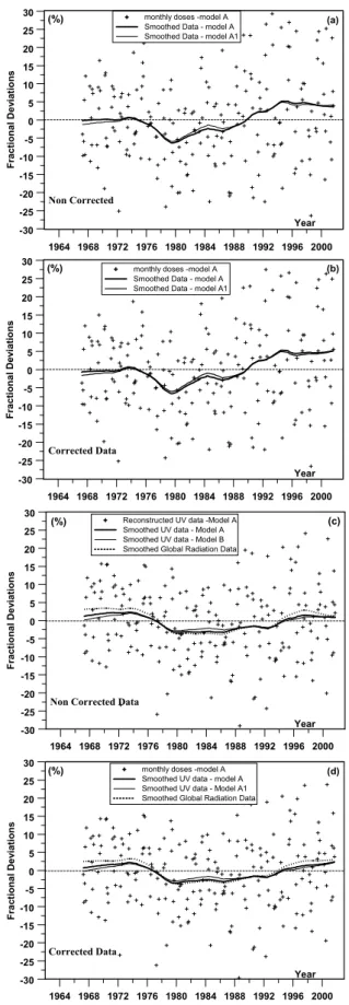
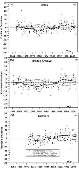
The reconstructed time series of UV fractional deviations calculated on a monthly basis for the April-September pe-riods are shown in Fig. 5 (Belsk), Fig. 6 (Hradec Kralove), and Fig. 7 (T˜oravere). Two categories of the time series are present – non-corrected (Fig. 5a, Fig. 6a, and Fig. 7a) and corrected (Fig. 5b, Fig. 6b, and Fig. 7b). The cloud-induced long-term variations are extracted from the reconstructed time series by repeating the model calculation (model A and A1) with a constant value of the monthly total ozone being equal to its long-term monthly mean. The results of the mod-els are shown for the non-corrected (Fig. 5c, Fig. 6c, and Fig. 7c) and corrected case (Fig. 5d, Fig. 6d, and Fig. 7d), superposed on the long-term pattern of fractional deviations of total solar radiation. The long-term total ozone effects on the UV level can be obtained in similar way, i.e. assuming constant values of CRF being equal to its long-term monthly

27 1 2 3 4 5 6 7 8 9 10 11 12 Month 0 4 8 12 0 4 8 12 (a) (MED) UV D ose Belsk Hradec Kralove Toravere 1 2 3 4 5 6 7 8 9 10 11 12 Month 0.6 0.7 0.8 0.9 1.0 0.6 0.7 0.8 0.9 1.0 U V T ransmittance Belsk Hradec Kralove Toravere (b)

Figure 4. The reconstructed seasonal pattern of the monthly mean dose (in MED unit) for

Belsk, Hradec Kralove and Toravere (a), and the cloud reduction factor over these stations (b)

for the period 1967-2001.

Fig. 4. The reconstructed seasonal pattern of the monthly mean dose (in MED unit) for Belsk, Hradec Kralove and Toravere (a), and the cloud reduction factor over these stations (b) for the period 1967–2001.

mean in the model calculations. We show (Fig. 8) results only for model A and for the corrected data because the over-all mean values of CRF by model A and A1 are almost equal also being independent of the data category, non-corrected or corrected. The long-term oscillations of ozone fractional deviations are superimposed on the reconstructed UV time series to illustrate periods with positive and negative total ozone trends.

There is a common pattern in the UV variations forced by total ozone over all analyzed stations, a period with de-creased UV levels in the 70s and 80s, and a period with high UV intensity in the 60s and 90s. This was due to a negative total ozone trend beginning at the end of the the 70s and a stronger attenuation of solar radiation in 70s and 80s by clouds. The modulation of UV radiation by clouds is the most spectacular over Hradec Kralove, where clear-sky con-ditions frequently appeared in the mid 60 s and a tendency of the atmosphere cleaning (i.e. weaker UV attenuation by clouds) had begun in the mid 80s and is still continuing there. This tendency is also seen over Belsk and T˜oravere but is much weaker. Moreover, the trendless period in the cloud forcing has to be noted over these stations, beginning in the second half of the 90s.

1482 J. W. Krzy´scin et al.: Long-term variations of the UV-B radiation over Central Europe 28 1964 1968 1972 1976 1980 1984 1988 1992 1996 2000 Year -30 -25 -20 -15 -10 -5 0 5 10 15 20 25 30 Frac ti on al D ev ia tio n s

monthly doses -model A Smoothed Data -model A Smoothed Data -model A1

(b) Corrected Data (%) 1964 1968 1972 1976 1980 1984 1988 1992 1996 2000 Year -30 -25 -20 -15 -10 -5 0 5 10 15 20 25 30 Fr act io nal De vi at ions

monthly doses -model A Smoothed UV data - model A Smoothed UV data - model A1 Smoothed Global Radiation Data

(%) (c)

Non Corrected Data

1964 1968 1972 1976 1980 1984 1988 1992 1996 2000 Year -30 -25 -20 -15 -10 -5 0 5 10 15 20 25 30 Frac ti on al D ev ia tio n s

monthly doses -model A Smoothed UV data - model A Smoothed UV data - model B Smoothed Global Radiation Data

(%) (d) Corrected Data 1964 1968 1972 1976 1980 1984 1988 1992 1996 2000 Year -30 -25 -20 -15 -10 -5 0 5 10 15 20 25 30 F ractio nal D ev ia ti on s

monthly doses -model A Smoothed Data -model A Smoothed Data -model A1

Non Corrected Data

(a) (%)

Figure 5. The reconstructed monthly means (by model A) of UV fractional deviations and

their smoothed pattern (by model A and A1); for non-corrected data set (a) and corrected data

set (b) for Belsk. The cloud induced part of the reconstructed UV fractional deviations for

non-corrected (c) and corrected (d) data set superposed on the monthly fractional deviations

of measured total solar radiation. Curves represent smoothing by LOWESS.

Fig. 5. The reconstructed monthly means (by model A) of UV frac-tional deviations and their smoothed pattern (by model A and A1); for non-corrected data set (a) and corrected data set (b) for Belsk. The cloud induced part of the reconstructed UV fractional devia-tions for non-corrected (c) and corrected (d) data set superposed on the monthly fractional deviations of measured total solar radiation. Curves represent smoothing by LOWESS.

29 1964 1968 1972 1976 1980 1984 1988 1992 1996 2000 Year -30 -25 -20 -15 -10 -5 0 5 10 15 20 25 30 Fr act io nal De vi at ions

monthly doses -model A Smoothed UV data - model A Smoothed UV data - model A1 Smoothed Global Radiation Data

(%) (d)

Corrected Data

Figure 6. The same as Fig. 5 but for Hradec Kralove.

1964 1968 1972 1976 1980 1984 1988 1992 1996 2000 Year -30 -25 -20 -15 -10 -5 0 5 10 15 20 25 30 Fr act io nal De vi at ions

monthly doses -model A Smoothed Data -model A Smoothed Data -model A1

(%) (b) Corrected Data 1964 1968 1972 1976 1980 1984 1988 1992 1996 2000 Year -30 -25 -20 -15 -10 -5 0 5 10 15 20 25 30 Fr act io nal De vi at ions

monthly doses -model A Smoothed UV data - model A Smoothed UV data - model A1 Smoothed Global Radiation Data

(%) (c)

Non Corrected Data

1964 1968 1972 1976 1980 1984 1988 1992 1996 2000 Year -30 -25 -20 -15 -10 -5 0 5 10 15 20 25 30 Fr act io nal De vi at ions

monthly doses -model A Smoothed Data -model A Smoothed Data -model A1

(%) (a)

Non Corrected

J. W. Krzy´scin et al.: Long-term variations of the UV-B radiation over Central Europe 1483 The long-term total ozone forcing on the UV radiation has

the same pattern over all considered stations, i.e. the increase in UV radiation due to a negative trend of total ozone in the 80s and the first half of the 90s, and a stabilization or even a slight decrease in the ozone-induced UV doses in the second half of 90s being a response to a trendless (or with a small positive trend) period in total ozone.

In analyzing the month-to month scatter of the monthly UV fractional departures (points in Figs. 5–8), it can be es-tablished that the cloud forcing is mostly responsible for month-to month variations in the surface UV monthly mean doses. The variance of the UV fractional deviations re-lated to the cloud forcing is ∼4 times greater than that due to total ozone variations for all considered stations. The monthly extreme departures are ∼−30% and ∼30% relative to the long-term monthly mean for extreme heavy clouds and sunny months, respectively, being also ∼2 times deeper and larger than those forced by extreme positive and negative to-tal ozone departures, respectively.

5 Conclusions

The reconstruction models examined here are capable of re-producing low-frequency variations of the monthly mean sur-face UV doses. This was supported by a reasonable agree-ment of the modeled and observed time series of the UV fractional deviations over Belsk for the period 1976–2001. A model separating the cloud and total ozone effects (Model A and A1 need a simulation of clear-sky doses with several assumptions of the input to radiative transfer model) and a sophisticated statistical model – MARS (model B) perform similarly when reconstructing the long-term monthly doses. MARS provides better simulations of daily variations of the UV doses over Belsk but it can be applied to other sites only if the UV-B has been measured there for a rather long period. MARS decreases significantly the degree of freedom of the regression, assuming many regression constants. In the case of the Belsk analysis, the number of constants is about 50, so at least twice the number of the data points is required to run effectively a MARS model (Friedman, 1991). Thus, when analyzing April–September monthly data (6 values per each year) it gives ∼15 years as a minimum length of the UV time series. Only such a long series enables one to achieve high accuracy of the UV simulations. MARS regression coeffi-cients are rather local ones and they should be determined individually for each site. There is no gain in the model per-formance if the MARS model is constructed for one place and used to simulate behaviour of UV series over other sites. Model A and A1 use the cloud reduction factor derived from the empirical formula parameterizing the reduction of the UV radiation by clouds from the reduction of total solar radiation. Our equation and that proposed by den Outer et al. (2000), to calculate the CRF dependence on SZA and total solar radia-tion yield almost the same result (see Figs. 5, 6 and 7). It is worth noting that those formulas were derived from the UV attenuation measurements over different places (Poland, and the Netherlands). Thus, their similar performance in the UV

30

Figure 7. The same as Fig. 5 but for Tõravere.

1964 1968 1972 1976 1980 1984 1988 1992 1996 2000 Year -30 -25 -20 -15 -10 -5 0 5 10 15 20 25 30 F ractio nal D ev ia ti on s

monthly doses -model A Smoothed Data - model A Smoothed Data - model A1

(%) (a) Non Corrected 1964 1968 1972 1976 1980 1984 1988 1992 1996 2000 Year -30 -25 -20 -15 -10 -5 0 5 10 15 20 25 30 Fr act io nal De vi at ions

monthly doses -model A Smoothed Data - model A Smoothed Data - model A1

(%) (b) Corrected Data 1964 1968 1972 1976 1980 1984 1988 1992 1996 2000 Year -30 -25 -20 -15 -10 -5 0 5 10 15 20 25 30 Frac ti on al D ev ia tio n s

Reconstructed UV data -Model A Smoothed UV data - Model A Smoothed UV data - Model B Smoothed Global Radiation Data

(%) (c)

Non Corrected Data

1964 1968 1972 1976 1980 1984 1988 1992 1996 2000 Year -30 -25 -20 -15 -10 -5 0 5 10 15 20 25 30 Frac ti on al D ev ia tio n s

monthly doses -model A Smoothed UV data - model A Smoothed UV data - Model A1 Smoothed Global Radiation Data

(%) (d)

Corrected Data

1484 J. W. Krzy´scin et al.: Long-term variations of the UV-B radiation over Central Europe

31

Figure 8. The reconstructed (model A) monthly means of the total ozone induced part of the

UV fractional deviations and their smoothed pattern (using LOWESS) for corrected data

superposed on the monthly fractional deviations of measured total ozone over Belsk (a),

Hradec Kralove (b), and Tõravere (c).

1964 1968 1972 1976 1980 1984 1988 1992 1996 2000 Year -30 -25 -20 -15 -10 -5 0 5 10 15 20 25 30 Fr act ion al Dev ia tio n s (%) _Belsk (a) 1964 1968 1972 1976 1980 1984 1988 1992 1996 2000 Year -30 -25 -20 -15 -10 -5 0 5 10 15 20 25 30 Fr ac tio n a l De viat io n s (%) _{Hradec Kralove} (b) 1964 1968 1972 1976 1980 1984 1988 1992 1996 2000 Year -30 -25 -20 -15 -10 -5 0 5 10 15 20 25 30 Fr act ion al Dev ia tio n s

monthly doses -model A Smoothed UV data - model A Smoothed Total Ozone Data

(%) _Toravere (c)

Fig. 8. The reconstructed (model A) monthly means of the to-tal ozone induced part of the UV fractional deviations and their smoothed pattern (using LOWESS) for corrected data superposed on the monthly fractional deviations of measured total ozone over Belsk (a), Hradec Kralove (b), and T˜oravere (c).

reconstruction supports their non-local properties and use-fulness in simulations of the UV doses for various conditions over many European sites. Our formula for SZA >72.5◦is proper for the more northern stations (with snow during win-ter time) but during snowless periods both formulas are al-most equivalent.

The reconstructed pattern of the UV radiation is as good as the level of homogeneity of the ancillary data used for the reconstruction. It is a difficult task to prepare a homoge-nized time series of total solar radiation (30–40 years) from observations carried out by various pyranometers. A full record of calibration changes and procedures applied

dur-ing those years are usually not available. We propose to run each reconstruction model separately for non-corrected and corrected time series of daily doses and daily sums of to-tal solar radiations. The model regression constants are also calculated separately for the non-corrected and corrected set of the variables. Thus, one realization of the model corre-sponds to the assumption that the data are perfect (no need for correction) and the second one implies the existing instru-mental drift (then the correction functions (1) and (2) were implemented). The UV climatology and long-term changes have been discussed using both time series. Fortunately, the total solar and total ozone observations carried out at all considered stations have been found proper for such long-term analysis. Using constant aerosols properties and wa-ter vapour content in the atmosphere from the NCEP/NOAA Reanalysis-2 data base lead to small fluctuations (with an amplitude of 2–3%, Fig. 1) in the long-term pattern of the model-observation differences. Thus, results obtained from both realizations of models could be easily synthesized.

The basic findings are: the latitudinal differences in the seasonal profiles (expected larger monthly doses for lower latitudes), similar climatological forcing by clouds for all considered stations, regional peculiarities in the cloud long-term forcing sometimes leading to extended periods with el-evated UV radiation (see strong and variable trends in the cloud induced UV variations over Hradec Kralove and much smaller trends over Belsk and T˜oravere with the same tem-poral pattern), recent stabilization of the ozone induced UV long-term change being a response to the trendless tendency of the total ozone since the mid 90s, and month-to-month variations in UV doses appeared to be mainly governed by the cloud variations.

Special attention to the long-term variations of the surface UV radiation has been triggered by an observed negative to-tal ozone trend since the mid seventies and an anticipated increase in the surface UV radiation thought to be harmful for the environment. Recently, the problem of the ozone recovery has been widely discussed and it seems that the total ozone trend is slowing down as a response to the de-creasing growth rate of man-made chlorine/bromine loading of the atmosphere. The reconstructed time series show that the UV level in the 60 s and early 70s was not much differ-ent than its presdiffer-ent level over Cdiffer-entral Europe for the April-September periods, i.e. for periods when normally the UV ra-diation is especially strong due to high solar elevation. Thus, we should pay more attention to the examination of sources of the cloud long-term and short-term variations. In case of slowdown of the total ozone trend over the Northern Hemi-sphere’s mid-latitudes and the anticipated the ozone recovery (WMO, 2003, Newchurch et al., 2003), clouds will appear as the most important modulator of the UV radiation both over long- and short-time scales during the next decades.

J. W. Krzy´scin et al.: Long-term variations of the UV-B radiation over Central Europe 1485 Acknowledgements. The study has been supported by the

Commis-sion of the European Communities through EDUCE project con-tract no. EVK2-CT-1999-00028 and by the State Inspectorate for Environment Protection, Poland, under contract no. 74/2003/F.

Topical Editor O. Boucher thanks two referees for their help in evaluating this paper.

References

Bojkov, R. D., Bishop L., and Fioletov V. E.: Total ozone trends from quality-controlled ground-based data (1964–1994), J. Geo-phys. Res., 100, 25 867–25 876, 1995.

Borkowski, J. L.: Homogenization of the Belsk UV-B time series (1976–1997) and trend analysis, J. Geophys. Res., 105, 4873– 4878, 2000.

Borderwijk, J. A., Slaper, H., Reinen H. A. J. M., and Schla-mann, E.: Total solar radiation and the influence of clouds and aerosols on the biologically UV, Geophys. Res.Lett., 22, 2151– 2154, 1995.

Cleveland, W. S.: Robust locally weighted regression and smooth-ing scatterplots, JASA, 74, 829–836, 1979.

de La Casini`ere, A., Tour´e, M. L., Masserot, D., Cabot, T., and Pinedo Vega, J. L.: Daily doses of biologically active UV radia-tion retrieved from commonly available parameters, Photochem-istry and Photobiology, 76, 171–175, 2002.

de Veaux, R., Gordon A., and Comiso J.: Modeling of topographic effects on Antarctic sea-ice using multivariate adaptive regres-sion splines, J. Geophys. Res.-Ocean, 98, 20 307–20 319, 1993a. de Veaux, R., Psichogios, R., and Ungar L. H.: A comparison of two nonparametric estimation schemes: MARS and neural networks, computers in chemical engineering, 17, 819–837, 1993b. den Outer, P. N., Slaper H., Matthijsen, J., Reinen, H. A. J. M.,

and Tax, R.: Variability of ground-level ultraviolet: Model and measurement, Radiat. Protect. Dosimetry, 91, 105–110, 2000. Eerme, K., Veismann, U., and Koppel, R.: Variations of erythemal

ultraviolet irradiance and dose at Tartu/T˜oravere, Estonia, Clim. Res., 22, 245–253, 2002.

Finizio, M. and Palmieri, S.: Non-linear modeling of monthly mean vorticity time changes; an application to the western mediter-ranean, Ann. Geophys., 16, 116–124, 1998.

Fioletov, V. E., McArthur, L. J. B., Kerr, J. B., and Wardle, D. I.: Long-term variations of UV-B irradiance over Canada estimated from Brewer observations and derived from ozone and pyra-nometer measurements, J. Geophys.Res., 106, 23 009–23 028, 2001.

Friedman, J. H.: Multivariate adaptive regression splines, The An-nals of Statistics, 19, 1–50, 1991.

Ito, T., Sakoda, Y., Uekuba, T., Naganuma, H., Fukoda, M., and Hayashi, M.: Scientific application of UV-B observation from JMA network, Proc. 13th UOEH Int. Symp. and the second PAN Pacific Cooperative Symp. On impact of increased UV-B expo-sure on human health and ecosystem, Kitakyushu, Japan, Univer-sity of Occupational and Environmental Health, 107–125, 1993. Janouch, M: UV Climatology–reconstruction and visualization of the UV radiation at the territory of Czech Republic, Proceedings of Quadrennial Ozone Symposium, Hokkaido University, Sap-poro, Japan, 3–8 July 2000, 235–236, 2000.

Jaroslawski, J., Krzy´scin, J. W., Puchalski, S., and Sobolewski, P.: On the optical thickness in the UV range: Analysis of the ground-based data taken at Belsk, Poland, J. Geophys.Res., 108(D23), 4722, doi:10.1029/2003JD003571, 2003.

Kaurola, J., Taalas P., Koskela T., Borkowski J., Josefsson W.: Long-term variations of UV-B doses at three stations in north-ern Europe, J. Geophys. Res., 105, 20 813-20 820, 2000. Kerr, J. B. and McElroy, C. T.: Evidence for large upward trends

of ultraviolet-B radiation linked to ozone depletion, Science 262, 1032–1034, 1993.

Krzy´scin, J. W.: UV controlling factors and trend derived from ground-based measurements at Belsk, Poland, 1976–1994, J. Geophys Res., 101, 16 797–16 805, 1996.

Krzy´scin, J. W.: Nonlinear (MARS) modelling of long-term vari-ations of surface UV-B radiation as revealed from the analysis of Belsk, Poland data for the period 1976–2000, Ann. Geophys., 21, 1887–1896, 2003.

Madronich, S.: Implications of recent total atmospheric ozone mea-surements for biologically active ultraviolet radiation reaching the surface, Geophys. Res. Lett., 19, 37–40, 1992.

Matthijsen, J., H., Slaper, H., Reinen, H. A. J. M., and Velders, G. J. M.: Reduction of solar UV by clouds: A comparison between satellite-derived clouds effects and ground-based measurements, J. Geophys. Res., 105, 5069–5080, 2000.

Mayer, B. and Seckmeyer, G.: All-weather comparison between spectral and broadband (Robertson-Berger) UV measurements, Photochem. Photobiol., 64, 792–799, 1996.

Newchurch, M. J., Yang, E.-S., Cunnold, D. M., Reinsel, G. C., and Zawodny, J. M.: Evidence for slowdown in stratospheric ozone loss: First stage of ozone recovery, J. Geophys. Res., 108 (D16), 4507, doi:10.1029/2003JD003471, 2003.

Ricchazzi, P., Yang, S., Gautier, C., and Sowle, D.: SBDART: A research and teaching tool for plane–parallel radiative transfer in the Earth’s atmosphere, Bull. Amer. Meteorol., Soc., 79, 2101– 2114, 1998.

Taliani, M., Palmieri, S., and Siani, A.: Visibility: An investigation based on a multivariate adaptive regression spline techniques, Meteorol. Appl, 3, 353–358, 1996.

Udelhofen, P. M., Gies, P., Roy C., and Randel, W. J.: Surface UV radiation over Australia, 1979–1992, Effects of ozone and cloud cover changes on variations of UV radiation, J. Geophys. Res., 104, 19 135–19 159, 1999.

Weatherhead, E. C., Tiao G. C., Reinsel G. C., Frederick J. E., de Luisi, J., Chou, D., and Tam, W.: Analysis of long-term be-haviour of ultraviolet radiation measured by Robertson-Berger meter at 14 sites in the United States, J. Geophys. Res., 102, 8737–8754, 1997.

Weatherhead, E. C., Reinsel, G. C., Tiao, G. C., Meng, X. L., Choi, D., Cheang, W.-K., Keller, T., de Luisi, J., Wuebbles, D. J., Kerr, J. B., Miller, A. J., Oltman, S. J., and Frederick, J. E.: Fac-tors affecting the detection of trends: Statistical considerations and applications to environmental data, J. Geophys. Res., 103, 17 149–17 161, 1998.

World Meteorological Organization (WMO), Scientific assessments of ozone depletion, 2002, ,WMO Ozone Report 47, Geneva, 498, 2003.

Zerefos, C. S, Bias, A. F., Meleti, C., and Ziomas, I. C.: A note on the recent increase of solar UV-B radiation over northern middle latitudes, Geophys. Res. Lett. 22, 1245–1247, 1995.