HAL Id: hal-00318183
https://hal.archives-ouvertes.fr/hal-00318183
Submitted on 20 Oct 2006
HAL is a multi-disciplinary open access
archive for the deposit and dissemination of
sci-entific research documents, whether they are
pub-lished or not. The documents may come from
teaching and research institutions in France or
abroad, or from public or private research centers.
L’archive ouverte pluridisciplinaire HAL, est
destinée au dépôt et à la diffusion de documents
scientifiques de niveau recherche, publiés ou non,
émanant des établissements d’enseignement et de
recherche français ou étrangers, des laboratoires
publics ou privés.
profiles close to local noon in the cusp
S. C. Robertson, B. S. Lanchester, M. Galand, D. Lummerzheim, A. B.
Stockton-Chalk, A. D. Aylward, I. Furniss, J. Baumgardner
To cite this version:
S. C. Robertson, B. S. Lanchester, M. Galand, D. Lummerzheim, A. B. Stockton-Chalk, et al.. First
ground-based optical analysis of H? Doppler profiles close to local noon in the cusp. Annales
Geo-physicae, European Geosciences Union, 2006, 24 (10), pp.2543-2552. �hal-00318183�
Ann. Geophys., 24, 2543–2552, 2006 www.ann-geophys.net/24/2543/2006/ © European Geosciences Union 2006
Annales
Geophysicae
First ground-based optical analysis of H
β
Doppler profiles close to
local noon in the cusp
S. C. Robertson1,2, B. S. Lanchester1, M. Galand3, D. Lummerzheim4, A. B. Stockton-Chalk1, A. D. Aylward2,
I. Furniss2, and J. Baumgardner5
1Space Environment Physics, University of Southampton, UK 2Atmospheric Physics Laboratory, University College London, UK 3Space and Atmospheric Physics Group, Imperial College London, UK 4Geophysical Institute, University of Alaska, USA
5Centre for Space Physics, Boston University, MA, USA
Received: 16 June 2006 – Accepted: 31 August 2006 – Published: 20 October 2006
Abstract. Observations of hydrogen emissions along
the magnetic zenith at Longyearbyen (78.2 N, 15.8 E geo-graphic) are used to investigate the energy and source of protons precipitating into the high latitude region. During the hours around local solar noon (11:00 UT), measurements of the hydrogen Balmer β line are severely affected by sun-light, such that most data until now have been disregarded during these times. Here we use a simple technique to sub-tract sunlight contamination from such spectral data. An ex-ample is shown in which the removal of twilight contamina-tion reveals a brightening of Hβ aurora over Svalbard on 27
November 2000 between 08:00 UT and 10:00 UT, which is centred on magnetic noon (08:48 UT). These data were mea-sured by the High Throughput Imaging Echelle Spectrograph (HiTIES), one instrument on the Southampton-UCL Spectro-graphic Imaging Facility (SIF). Data from the IMAGE satel-lite confirms the location of a cusp “spot” over Svalbard at the time of the ground-based measurements, which moved in response to changes in the IMF conditions. A coincident pass of the DMSP F12 satellite provided input spectra for modelling studies of the Hβ profiles, which confirm that the
method for removing the twilight contamination is robust. The results described here are the first ground-based optical measurements of Hβ Doppler profiles from the cusp region
close to local solar noon, when scattered sunlight swamps the raw data.
1 Introduction
Auroral hydrogen emissions are the spectroscopic signature of energetic proton precipitation into the atmosphere. Hy-drogen line profiles measured from the ground provide
in-Correspondence to: B. S. Lanchester
formation about the processes that protons undergo as they propagate through the upper atmosphere (e.g. Lummerzheim and Galand, 2001). In particular, spectrographic measure-ments using CCD detectors allow the whole wavelength range of the Doppler shifted profile of H emissions to be recorded simultaneously. Given sufficient wavelength res-olution (0.13 nm herein), these profiles can be combined with modelling studies to determine the energy spectrum and energy flux of the incoming hydrogen, and hence gain in-sight into the source of the protons (Galand and Chakrabarti, 2006).
There is particular interest in the emissions resulting from proton precipitation in the region of the cusp, where these emissions are the unique signature of protons that have gained direct access to the Earth’s ionosphere along newly reconnected field lines at the magnetopause. It should be noted that protons are more suitable than electrons for pro-viding information on solar wind-magnetosphere coupling, as they are less sensitive than electrons to magnetospheric processes, and retain information on their source. The tem-poral and spatial variations of H emissions in the region in or near the cusp have been highlighted in the many results in recent years from the Spectrographic Imager (SI12)/FUV in-strument on the Imager for Magnetopause-to-Aurora Global Exploration (IMAGE) satellite, which provides 5–10 s im-ages of the Doppler-shifted integrated Lyman-α emission at 2 min intervals of the entire auroral oval (Mende, 2000). This emission, like the Doppler-shifted Hβ emission, is produced
solely by proton precipitation into the atmosphere. In a sta-tistical survey of cusp aurora, Frey et al. (2002) used IMAGE data to study the behaviour of a region of intense Lyman-α emission poleward of the oval, making estimates of both the electron and proton energy fluxes at the times of occurrence of the “spot”. As the SI12 does not provide spectral infor-mation, the estimate of proton flux is limited by the choice made for the energy of the incident protons. While the spatial
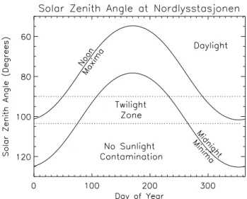
Fig. 1. The solar zenith angle (SZA) at Nordlysstasjonen over a
year at noon (upper curve) and midnight (lower curve). The two horizontal dotted lines give the SZA range 90◦to 103.5◦over which twilight contamination is observed.
resolution of this instrument is low (50 km) compared with ground based measurements, it provides an invaluable mea-sure of the magnetospheric context within which to place high resolution spectrographic observations.
Ground-based measurements of hydrogen emissions in the region of the cusp have long been made from Svalbard (75◦ magnetic latitude). Ebert–Fastie spectrophotometers scan-ning over wavelength in time were used to study hydro-gen line profiles by Henriksen et al. (1985); Sigernes et al. (1994); Sigernes (1996); Lorentzen et al. (1998) and Deehr et al. (1998). However, as detailed by Henriksen et al. (1985), the effects of Rayleigh scattering are a limiting factor for dayside optical observations, especially for the Hβ line. All
the above published measurements of hydrogen emissions near local noon are of the Hα line, which suffers less from
Rayleigh scattering because of the λ−4dependence. Henrik-sen et al. (1985) show examples of zenith spectra taken 3 h before local noon in late January at Svalbard, in the wave-length regions around both the Hα and Hβ lines during an
exceptionally strong proton aurora. The Hαspectrum shows
a clear line profile, but the Hβ spectrum is dominated by
the Fraunhofer absorption line. Henriksen et al. (1985) con-cluded that there is a significant contribution from Rayleigh scattered sunlight on zenith observations of both Hα and Hβ
at solar depression angles less than approximately 10◦ and 13◦, respectively.
The advent of CCD detectors into the field of spectroscopy has provided the means to increase sensitivity as well as resolution in wavelength and time. Such imaging spec-trographs are currently the optimal instruments for high spectral resolution measurements of auroral hydrogen lines
(Baumgardner et al., 1993). The High Throughput Imaging Echelle Spectrograph (HiTIES), the main instrument on the Spectrographic Imaging Facility (SIF) in Nordlysstasjonen on Svalbard is well documented (Chakrabarti et al., 2001; McWhirter et al., 2003; Lanchester et al., 2003; Galand et al., 2004). Nordlysstasjonen is located at geographic 78.2 N and 15.8 E, which corresponds to a local noon at 10:56:48 UT. At this latitude, the Sun is below the horizon between 27 Oc-tober and 15 February. Between 14 November and 29 Jan-uary the Sun does not rise higher than 6◦ below the hori-zon, and daytime measurements are possible. However, twi-light contamination around local noon can be up to three or-ders of magnitude brighter than the proton induced aurora. Figure 1 shows the solar zenith angle from Nordlysstasjo-nen over a year. Twilight emission is detected in HiTIES measurements between solar zenith angles 90◦ and 103.5◦,
marked in the figure to delineate times of direct sunlight, twilight, and night. This diagram shows that even at mid-winter, several hours of auroral observation time are severely affected each day by twilight contamination.
In this paper we have applied a simple method to re-move the effects of twilight from measured Hβ profiles.
This method is described in Sect. 2 and applied to H emis-sion Doppler profiles acquired from the HiTIES spectrograph from Svalbard near local noon. A case study of proton in-duced aurora on 27 November 2000 is presented in Sect. 3. The subtraction method reveals a significant region of un-derlying Hβ emissions, which changed temporally and
spa-tially in response to changes in the solar wind. Measurements from the ACE and IMAGE satellites are used to place the ground-based measurements in the context of the large-scale events. In Sect. 4, energy spectra from the DMSP F12 satel-lite are used as input to modelling, in order to compare the shape of the Hβ profiles that are extracted from the
twilight-contaminated data with those produced by the model.
2 Twilight contamination
As seen in Fig. 1 there is contamination from sunlight around local noon even at midwinter. The twilight contamination in HiTIES data can be written as
T (λ) = ST(λ) + AT(λ) (1)
where (ST) is Rayleigh scattered sunlight and (AT) is made
up of other minor atmospheric emissions. Most of the con-tamination is scattered sunlight, given by
ST(λ) = F (λ) × σR(ς ) (2)
where F (λ) is the Fraunhofer spectrum, ς is solar zenith an-gle, and σRis the Rayleigh scattering function, inversely
pro-portional to λ4. Wavelength dependent effects are considered negligible over the 4 nm filter range.
S. C. Robertson et al.: Hβprofiles near noon in the cusp 2545
Fig. 2. Spectrum (T (λ)) recorded by HiTIES between 08:45 UT
and 10:01 UT on 30 November 2002.
The smaller secondary component is atmospheric emis-sion from a number of sources:
AT(λ) = ASD(λ) + ASI(λ) + C(λ) + P (λ) (3)
where ASD(λ) is from direct sunlight excitation, ASI(λ)
is from scattered sunlight and secondary emission due to
ASD(λ) emission, C(λ) is emission due to atmospheric
chemistry and P (λ) is emission resulting from auroral exci-tation. These emissions exist over the whole HiTIES spec-trum, and have a range of radiative lifetimes. Modelling
AT(λ)is made difficult by lack of experimental results on the
minor atmospheric emission species. The auroral Hβline lies
between 483 nm and 487 nm. We here assume that AT(λ)
does not vary with wavelength over this range, but varies di-rectly with solar input, such that
AT(λ) = A(ς ) (4)
This assumes no long radiative lifetime or chemically driven emissions are present in the band, which is not contradicted by the data. This approximation also assumes there are no auroral emissions other than Hβ in the band. Therefore
T (λ) = F (λ) × σR(ς ) + A(ς ) (5)
The overall shape of the twilight contamination spectrum does not vary, but its magnitude varies as a function of ς and atmospheric opacity. The shape of the atmospheric spectrum during twilight is shown in Fig. 2. No auroral emission was detected by the instruments at Nordlysstasjonen during the integration period of this spectrum (08:45 UT to 10:01 UT on 30 November 2000). The twilight brightness, including the effect of atmospheric opacity, is now estimated by nor-malising the solar spectrum to the background emission level of the data spectrum. The wavelength range selected as the
Fig. 3. An example Hydrogen β profile. The shaded area indicates
the chosen background region of the spectrum.
background area in the Hβfilter, , is shown in Fig. 3, which
is a data sample taken when there was no daylight contami-nation. This shows that the background is well clear of the Hβred wing. The normalising factor is therefore given by
φ = D T
(6)
where D is the background brightness level of the data
spectrum, and T is the background brightness level of the
reference twilight spectrum. Note that maximising the wave-length range over which the background is measured min-imises the error in φ. At the time that these data were taken, the wavelength range selected for the filter gave the red wing of the Hβ line good clearance at the high wavelength end,
and hence a good background sample range.
Taking a twilight contaminated data spectrum, D(λ), the twilight can be estimated using the reference twilight spec-trum T (λ) and the scaling constant φ (Eq. 6). This estimate can then be subtracted from D(λ) to reveal the underlying spectrum (R(λ)).
R(λ) = D(λ) − φT (λ) (7)
Figures 4–6 show examples of the twilight estimation pro-cess and the resulting subtracted spectra. These will be dis-cussed in more detail in Sect. 3. The process estimates and subtracts T (λ) accurately, to reveal the much smaller under-lying hydrogen profile, R(λ). Note that R(λ) still has the Poisson variance of the larger initial spectrum after the sub-traction.
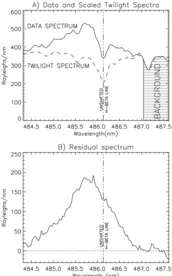
Fig. 4. (A) A measured spectrum (solid line), integrated for 60 s
beginning at 09:06:34 on 27 November, 2000. The φ-scaled twi-light spectrum is drawn as a dashed line. (B) The residual spectrum after the scaled twilight spectrum has been subtracted from the data spectrum.
3 Observations
3.1 Overview
The present observations were made following a period of exceptional solar activity, with eruptions of four halo Coro-nal Mass Ejections (CMEs) within 18 h on 24–25 November, 2000. On 27 November 2000, the solar wind velocity was raised (≈600 km/s) for a period of about 8 h before the event described here. Both ACE and Wind satellites registered sud-den increases in proton number sud-density from 20 to 50 cm−3. A time lag of about 41 min for this increase in solar wind pressure to reach the magnetopause has been estimated using a method described in Lockwood et al. (2003), which uses both ACE and Wind positions at the time of the increase.
Fig-Fig. 5. (A) A measured spectrum (solid line), integrated for 60 s
beginning at 09:21:57 UT on 27 November, 2000. The φ-scaled twilight spectrum is drawn as a dashed line. (B) The residual spec-trum after the scaled twilight specspec-trum has been subtracted from the data spectrum.
ure 7 is the ACE data lagged by this interval and plotted be-tween 07:30–10:00 UT, which correspond to estimated times of arrival of the measured changes in solar wind parameters at the magnetopause. The density increase can be seen in the second panel at approximately 08:30 UT. The magnetic field components in Geocentric Solar Magnetospheric (GSM) co-ordinates are plotted in the lowest three panels. Following the density increase the magnetic field Bzchanges from close to
zero to positive (>20 nT), and By, having been strongly
pos-itive (20 nT) at the time of the increase in solar wind pres-sure, subsequently becomes strongly negative (−20 nT). At the same time Bzreturns to almost zero. Three arrows mark
the significant changes in the solar wind parameters which result in observable effects in the ionosphere.
S. C. Robertson et al.: Hβprofiles near noon in the cusp 2547
Fig. 6. (A) A measured spectrum (solid line), integrated for 60 s
beginning at 09:25:22 UT on 27 November, 2000. The φ–scaled twilight spectrum is drawn as a dashed line. (B) The residual spec-trum after the scaled twilight specspec-trum has been subtracted from the data spectrum.
The IMAGE satellite was well located to provide an ex-cellent overview of the large-scale changes in the auroral UV emissions related to the above changes in the solar wind. The first sign of the arrival of the pressure pulse generated by the increase in proton density is seen at 08:32:43 UT with a brightening of a region of Lyman-α emission centred at 14:30 MLT, in excellent agreement with the lag estimated and plotted in Fig. 7. This “spot” continues to fluctuate in in-tensity with a peak at 09:03:23 UT when it is centred closer to magnetic noon, but still duskward. During this time the oval is contracting poleward from an initially large area, re-sulting from earlier negative Bz. By 09:32 UT the spot is
centred at noon well poleward of the main oval and is over Svalbard. After this, the effect of the change in By is seen
V (km/s) 600 650 N (/cm 3 ) 20 40 60 B x (nT) −20 0 20 B y (nT) −20 0 20 B z (nT) UT (hrs:mins)+lag 8:00 8:30 9:00 9:30 10:00 −20 0 20
Fig. 7. Data from the ACE satellite for 27 November, 2000, lagged
by 41 min. Arrows mark the times of significant changes that result in observed effects in the ionosphere.
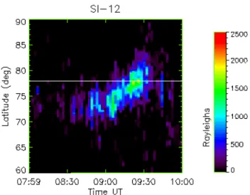
Fig. 8. Time history of IMAGE Lyman-α intensity at longitude of
Longyearbyen. The horizontal line marks the latitude of Longyear-byen.
clearly as the spot moves dawnwards of noon, such that by 10:00 UT it is centred at 11:00 MLT (about 2 h MLT from Svalbard).
The spatial and temporal changes in Lyman-α brightness over Longyearbyen are shown in Fig. 8, which is a time sequence of latitude slices centred on longitude 16.0◦ and averaged over 2◦ in longitude. The geographic latitude of Longyearbyen is marked with a horizontal line. The figure confirms the presence of the intense proton aurora over Sval-bard between 09:20 UT and 09:35 UT. Two Lyman-α images
Fig. 9. IMAGE Lyman-α spectrograph data at 09:23:50 UT plotted
in magnetic latitude and magnetic local time coordinates. The F12 footprint is drawn with a thin line and its position at this time is marked with an asterisk.
Fig. 10. As for Fig. 9 at 09:25:53 UT.
from the SI12 instrument at 09:23:50 UT and 09:25:53 UT, at the peak brightness of the event measured from the ground, are shown in Figs. 9 and 10. They also show the position of the DMSP F12 satellite as it crossed the region. Particle data from this pass are used in Sect. 4. At these times the cusp spot is still centred on the duskward side of 12:00 MLT, with most intensity poleward of the main auroral oval.
3.2 Ground-based optical measurements
Sunlight contamination has been removed from the HiTIES Hβprofiles for the interval between 08:00 UT and 10:00 UT,
and these are shown as a time series in the bottom panel of Fig. 11. The integrated brightness over the whole Hβ
spectrum is shown in the top panel. Significant Hβ
emis-sion was first observed soon after 08:30 UT and continued through local magnetic noon (08:48 UT). HiTIES sees the largest emissions between 09:18 UT and 09:35 UT,
confirm-Fig. 11. (top) Changes in peak Hβ intensity. (bottom) Changes in
Hβprofile intensities.
ing IMAGE/SI12 observations over Svalbard (Fig. 8). The solar contamination was already strong by 09:00 UT and by the end of the interval was two orders of magnitude larger than the Hβ brightness. Three example plots are shown in
Figs. 4–6 for the times 09:06 UT at the start of the event, and 09:22 UT and 09:25 UT. The Doppler shifted hydrogen pro-file is clearly present. The maximum integrated brightness of 750±250 R occurred at 09:25 UT. The short wavelength end of the spectra shows some variability which could be contaminating auroral emissions from the N2Vegard-Kaplan
(2,15) band. The effects of such emissions on the analysis are discussed in Sect. 4. The full analysis of the errors in the data from HiTIES can be found in Robertson (2006).
4 Modelling of Hβprofiles
In order to derive Doppler profiles of radiating hydrogen atoms, it is necessary to solve the equations for the trans-port of fast protons into the atmosphere, their energy degra-dation and scattering, and their conversion to neutral atoms. The present work adopts the Galand et al. (1998) model which takes into account the collisional angular redistribu-tion through elastic collisions and through charge-changing collisions (i.e., capture and stripping). Starting with an in-cident proton beam, the resulting H emission Doppler pro-files are determined from the computed particle intensities, neutral densities and emission cross-sections. Since the pro-ton/H atom intensities in the upper atmosphere are directly proportional to the energy flux of the incident proton beam, the Hβ Doppler profile is also proportional to the energy flux
S. C. Robertson et al.: Hβprofiles near noon in the cusp 2549
of the incident proton beam. The detailed shape depends on the precipitating proton energy spectrum and pitch angle dis-tribution. A full description of the model is given in Galand et al. (1998) and Lanchester et al. (2003). The latter contains examples of model results compared with HiTIES measured profiles and an appendix with a full description of the model equations.
At the time of the brightest feature measured over Longyearbyen there was a close passage of the DMSP F12 satellite. Its footprint and position at the times of two consecutive images are marked in Fig. 9 and Fig. 10, when Svalbard was directly beneath the cusp spot. As F12 travelled through the cusp region, the measured differential energy flux of protons (not shown) was increased for energies above 100 eV up to the maximum energy measured by the satellite of 30 keV. The electron differential energy flux was also increased for energies between 100 eV and 1 keV. Three ion energy spectra typical for the data acquired during the Svalbard overpass have been selected as input to the model. Above the cut-off energy of the DMSP ion spectrometer (30 keV) we have extrapolated the particle flux logarithmically to 100 keV in all three cases. For the ion data at 09:24:10 UT and 09:25:00 UT the input spectra have also been generated with a sharp cut-off at 30 keV for an estimation of the sensitivity of the Hβ profiles to the high
energy tail. These input spectra are shown in the top panel of Fig. 12. The energy flux Q0and mean energy Emin each
case are: time shape Q0 Em (UT) (mW m−2) (keV) 09:24:10 extrapol 100 keV 1.6 2.7 09:24:10 sharp tail 1.2 2.0 09:24:30 extrapol 100 keV 2.8 3.0 09:25:00 extrapol 100 keV 3.2 4.0 09:25:00 sharp tail 2.2 2.8
The corresponding model profiles calculated along the magnetic zenith for the five input spectra are plotted in nor-malised form in the lower panel of Fig. 12. The instru-ment spectral resolution of 0.13 nm has been convolved with the model results. It can be seen that the high energy tail has a small effect on the short wavelength wing of the pro-files, with the most raised wing corresponding to the log-arithmically extrapolated spectrum at 09:25:00 UT. A dis-tinct effect is seen in the shape of the profiles for input spec-tra with larger fluxes around 1–10 keV, most evident in the 09:24:30 UT spectrum. This results in a broadening of the Hβprofile around 485.5 nm.
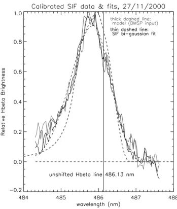
The model profile resulting from the F12 input spectrum at 09:25 UT has been chosen for comparison with four profiles measured between 09:22–09:26 UT in Fig. 13. The model profile (thick dashed line) is scaled to fit approximately to the
10−1 100 101 102
100 102 104
Energy (keV)
Incident proton flux (cm
−2 s −1 eV −1 sr −1 )
27 November, 2000 − DMSP particle data
092410: log extrapol to 100 keV 092410: sharp tail
092430: log extrapol to 100 keV 092500: log extrapol to 100 keV 092500: sharp tail 4840 484.5 485 485.5 486 486.5 487 0.2 0.4 0.6 0.8 1 Wavelength (nm)
Emission rate (arbitrary units)
Hβ magnetic zenith Doppler profile
Fig. 12. (top) DMSP F12 input ion fluxes with and without high
energy extrapolation. (bottom) Doppler-shifted Hβ profiles along
the magnetic zenith resulting from the H+/H model driven by the DMSP input spectra above.
peak of the measured profiles. The overall shapes of both the modelled and the observed Hβ Doppler profiles are similar.
The solar subtraction appears to be very slightly overdone, such that there is a dip in the long wavelength or “red” wing of the profile corresponding to the position of the Fraun-hofer absorption line. The main difference is in the raised short wavelength or “blue” wing, which is underestimated by the model results. This underestimation is not surpris-ing as it corresponds to an underestimation of the energy spectra above the DMSP energy cut-off. As the observed Hβ emission event is associated with a significant pressure
pulse, it is very probable that protons of high energy (above 30 keV) have flux larger than usual. As mentioned above, there may be electron induced auroral emission from the N2
VK band. There is no way currently of estimating the ex-tent of such emission during twilight hours, but it could have the effect of increasing the background to be subtracted at short wavelengths, and therefore reducing the height of the measured blue wing. The blue wing may also be affected
Fig. 13. Comparison of measured (solid lines) and modelled (thick
dash) Hβ profiles. The thin dashed line is a fit to the measured
profiles.
by the presence of patchy cloud, which would scatter Hβ
into the detector from other parts of the sky, producing a more symmetric profile. Also, if a background measurement had been possible shortward in wavelength of the H emis-sion profile, this may have reduced the blue wing further. Different mosaic filters have subsequently been designed for HiTIES that make this a possibility in future daytime mea-surements. While the comparison of the modelled profiles with the HiTIES data is limited above 30 keV due to the lack of particle data at the top of the atmosphere, the comparison with the model confirms the shape of the profiles below this energy. The model results have previously been validated against observed Hβ profiles of proton aurora in dark sky
conditions (Lanchester et al., 2003; Ivchenko et al., 2004).
5 Discussion
Changes in the brightness and position of hydrogen emis-sions in the region of the cusp reveal much about the re-connection processes which allow protons to precipitate into the high latitude ionosphere. For the events of 27 November 2000, described here, there was a particularly high density of protons in the solar wind, following a string of halo CMEs a few days before. From the lagged solar wind measurements shown in Fig. 7 it can be seen that an increase in proton den-sity was estimated to arrive at the magnetopause just after
08:30 UT. The lag can only be estimated to within ±3 min; the arrival of the pressure pulse is clearly seen at 08:33 UT on the ground by HiTIES, and by the IMAGE spectrographs, confirming that the plotted lag of 41 min is a good prediction. At this time the IMF was almost entirely in the positive By
direction. The reconnection site under this condition is pre-dicted to be at high latitudes on the dusk side of noon in the northern hemisphere for anti-parallel reconnection (Crooker, 1979; Luhmann et al., 1984; Chisham et al., 2002). Both the SI12 Lyman-α measurements as well as those from the SI13 imager confirm that precipitation has occurred in the post-noon sector, with increased brightness of emissions. The lat-ter are associated predominantly with OI 135.6 nm oxygen emission, which could be either from primary precipitating electrons, or indirectly from secondary electrons produced by protons and hydrogen atoms as they precipitated. The F12 electron energy spectra confirm that there were indeed precipitating electrons in the energy range 100 eV to 1 keV in this region. The study of the relative importance of pro-tons and electrons in such a reconnection event is an impor-tant subject, but it is not addressed further here. Analysis of the large-scale hydrogen and electron aurora and associated ionospheric flows during this interval will be presented in a separate paper.
Before the arrival of the pressure pulse and its manifesta-tion as a bright spot duskward of noon, the auroral oval was particularly large, following a time of negative Bz. The
pro-ton spot appears first within the main oval. As the IMF Bz
increases, the spot brightens and is seen poleward of the oval and closer to noon at 08:47 UT. The oval contracts steadily thereafter during the period of positive Bzand a steady
de-crease of By to zero. The next effect that is seen is the
sud-den change to purely negative By, during which time the spot
moves rapidly to pre-noon. These changes correspond to the reconnection site moving through higher latitudes across the noon meridian (when the IMF was in positive Bzdirection),
to the opposite lobe on the pre-noon magnetopause. The lon-gitudinal shift of the cusp may be enhanced by the distor-tion of magnetospheric field lines by IMF By(Cowley et al.,
1991). The changes in latitude of the spot in Lyman-α can be seen over Svalbard in Fig. 8. At the start of the interval, the oval is south of Svalbard, and the first significant increase in brightness is seen at about 73◦N geographic latitude just after 08:30 UT. The contraction of the oval follows, with the brightest and most northerly emissions seen at 09:25 UT over Svalbard at 78◦N latitude, corresponding to the time of
max-imum Bz. After that the spot moves away to pre-noon and
Svalbard also rotates even further way from noon in the op-posite sense. The region of emission moves slightly equator-ward again as the IMF Bzreturns to zero. This behaviour of
the cusp spot is consistent with previous studies, for example Milan et al. (2000), who used FUV measurements from the Polar satellite to study the response of dayside emissions to changes in IMF direction, during predominantly northward IMF.
S. C. Robertson et al.: Hβprofiles near noon in the cusp 2551
From the ground, measurements of Hβ Doppler profiles
provide information about the changes to the energy of the incoming protons. We use a simple fitting process to es-timate the changes in the shape and in the peak brightness and wavelength of the peak. The method is described fully by Lummerzheim and Galand (2001). A synthetic line pro-file is constructed from a Gaussian shape with different half widths on the short and long wavelength sides of the peak, thus accounting for the different Doppler shift produced by precipitation towards the instrument and scattering of hy-drogen away from the instrument, respectively. These syn-thetic spectra are fitted to the measured profiles, using a nonlinear least squares fitting method. A sample fitted pro-file is drawn as a thin dashed line in Fig. 13. The changes in blue wing halfwidth and peak wavelength (not shown) are not large, although there is a slight trend to larger blue shift with time between 09:05 and 09:35 UT. Previous re-sults (Lanchester et al., 2003) from the afternoon oval have found that changes in the blue wing correspond to chang-ing energy distributions associated with the large scale move-ment of the proton precipitation region over the ground sta-tion. The blue wing halfwidth of these previous measure-ments from Longyearbyen range between 0.6 and 1.0 nm, extending higher than but overlapping with the values mea-sured here (0.6–0.8 nm), whereas those meamea-sured at lower latitudes (in the afternoon/evening sector of the auroral oval) have been found to have a greater blue wing extent of up to 2.0 nm (Galand et al. (2004) and references therein). There is no strong evidence here of a velocity filter in operation as described in Deehr et al. (1998). Their observation co-incided with an equatorward motion of the dayside aurora, and therefore was the result of different processes from those observed here, where the brightest emissions occur at a time of northward IMF, and the subsequent combination of a sud-den change in IMF By and the rotation of the earth moved
the cusp precipitation abruptly away from our ground sta-tion. Careful consideration of spatial and temporal changes is crucial when interpreting ground-based data. Here the mo-tion of the emission region relative to Svalbard is a mixture of changes in both latitude and longitude, which makes inter-pretation of the event complicated.
6 Summary
The purpose of this paper is to demonstrate that Hβ profiles
measured during twilight hours can be used in the study of cusp daytime precipitation. The profiles have been extracted from data that would normally have been rejected because of the contamination from scattered sunlight. The fortuitous pass of the DMSP F12 satellite on 27 November 2000, co-incided with the time that the By component of the IMF
was changing from strongly positive to strongly negative, and thus just as the proton induced auroral spot was about to move to its pre-noon position. It also coincided with the
time of brightest Hβ measured at Svalbard. The ion energy
spectra measured by F12 are therefore very suitable as in-put for modelling. The comparison of modelled profiles with the data is limited by the low energy cut-off of the ion de-tector (30 keV). The high energy ion spectral tail has been extrapolated logarithmically up to 100 keV, which is a plau-sible guess but remains arbitrary. Closer fits of the model to the data at large blue shifts could possibly be made by changing the high energy tail. The comparison is also lim-ited by uncertainties in differential cross sections. The width of the spectrum at half maximum fits well, but it can be seen from the different model results that small variations will oc-cur with changes to the energy flux and mean energy in this region. Although the F12 satellite passed close to Longyear-byen, it did not pass exactly over the ground site, so differ-ences in this region of the profile would be expected. There is evidence that the background subtraction could be refined still further, if the effect of electron auroral emissions can be estimated, and with the inclusion of background subtraction from the short wavelength end of the spectrum.
We were also fortunate to have data from IMAGE with which to compare the ground-based measurements. These confirm that the cusp precipitation resulted from the observed changes in the IMF. In future, using this technique, Hβ
pro-files during daytime can be used to reveal the signature of proton precipitation, and therefore extract information about the energy flux and mean energy of the protons by comparing the profiles with model results. No clear dispersion signa-ture was observed in the cusp protons, but this is not surpris-ing given the sudden movement of the cusp emission region away from Svalbard at the time of maximum intensity. This combination of ground-based measurements and modelling provides a method of detecting changes in energy that re-sult from dayside reconnection, both at low latitudes (Deehr et al., 1998), and in the high latitude lobe regions as seen here. The use of more than one spectrograph on the ground in the cusp would be of great benefit to this study as sug-gested by Deehr et al. (1998).
Acknowledgements. The DMSP particle detectors were designed
by D. Hardy of AFRL, and data obtained from JHU/APL. The au-thors thank D. Hardy, F. Rich and P. Newell for its use, and in partic-ular F. Rich for providing data specific to our needs. ACE and Wind data were obtained from CDAWeb and we acknowledge the follow-ing PIs: D. J. McComas, R. Leppfollow-ing and K. Ogilvie. Thanks are offered to H. Frey for supplying the IMAGE data and for help with data reduction. The research was supported by the PPARC in the UK which also funded the spectrograph. M. Galand was supported in part by NASA grant NAG5-12773, D. Lummerzheim by NASA grants NAG5-11694 and NAG5-12192. We acknowledge with grat-itude the help given in this work by the late N. Shumilov.
Topical Editor M. Pinnock thanks C. Deehr and B. V. Kozelov for their help in evaluating this paper.
References
Baumgardner, J., Flynn, B., and Mendillo, M.: Monochromatic imaging instrumentation for applications in aeronomy of the earth and planets, Optical Eng., 32, 3028–3032, 1993.
Chakrabarti, S., Pallamraju, D., Baumgardner, J., and Vaillancourt, J.: HiTIES: A High Throughput Imaging Echelle Spectrograph for ground-based visible airglow and auroral studies, J. Geophys. Res., 106, 30 337–30 348, 2001.
Chisham, G., Pinnock, M., Coleman, I. J., Hairston, M. R., and Walker, A. D. M.: An unusual geometry of the ionospheric sig-nature of the cusp: implications for magnetopause merging sites, Ann. Geophys., 20, 29–40, 2002,
http://www.ann-geophys.net/20/29/2002/.
Cowley, S. W. H., Morelli, J. P., and Lockwood, M.: Dependence of convective flows and particle precipitation in the high-latitude dayside ionosphere on the X and Y components of the interplan-etary magnetic field, J. Geophys. Res., 96, 5557–5564, 1991. Crooker, N. U.: Dayside merging and cusp geometry, J. Geophys.
Res., 84, 951–959, 1979.
Deehr, C. S., Lorentzen, D. A., Sigernes, F., and Smith, R. W.: Dayside auroral hydrogen emission as an aeronomic signature of magnetospheric boundary layer processes, Geophys. Res. Lett., 25, 2111–2114, 1998.
Frey, H. U., Mende, S. B., Immel, T. J., Fuselier, S. A., Claflin, E. S., Gerard, J.-C., and Hubert, B.: Proton aurora in the cusp, J. Geophys. Res., 107, A7, doi:10.1029/2001JA900161, 2002. Galand, M., Lilenstein, J., Kofman, W., and Lummerzheim, D.:
Proton transport model in the ionosphere: 2, Influence of mag-netic mirroring ad collisions on the angular redistribution in a proton beam, Ann. Geophys., 16, 1308–1321, 1998,
http://www.ann-geophys.net/16/1308/1998/.
Galand, M., Baumgardner, J., Pallamraju, D., Chakrabarti, S., Lovhaug, U. P., Lummerzheim, D., Lanchester, B. S., and Rees, M. H.: Spectral imaging of proton aurora and twi-light at Tromso, Norway, J. Geophys. Res., 109(A7), A07305, doi:10.1029/2003JA010033, 2004.
Galand, M. and Chakrabarti, S.: Proton aurora observed from the ground, J. Atmos. Ter. Phys., 68, 1488–1501, 2006.
Henriksen, K., Fedorova, N. I., Totunova, G. F., Deehr, C. S, Romick, G. J., and Sivjee, G. G.: Hydrogen emissions in the polar cleft, J. Atmospheric Terr. Phys., 47, 1051–1056, 1985. Ivchenko, N., Galand, M., Lanchester, B. S., Rees, M. H.,
Lum-merzheim, D., Furniss, I., and Fordham, J.: Observation of O+(4P −4D0)lines in proton aurora over Svalbard, Geophys. Res. Lett., 31, L10807, doi:10.1029/2003GL019313, 2004.
Lanchester, B. S., Galand, M., Robertson, S. C., Rees, M. H., Lum-merzheim, D., Furniss, I., Peticolas, L. M., Frey, H. U., Baum-gardner, J., and Mendillo, M.: High resolution measurements and modelling of auroral hydrogen emission line profiles, Ann. Geo-phys., 21, 1629–1643, 2003,
http://www.ann-geophys.net/21/1629/2003/.
Lockwood, M., Lanchester, B. S., Frey, H., Throp, K., Morley, S., Milan, S. E., and Lester, M.: IMF Control of Cusp Proton Emis-sion Intensity and Dayside Convection: implications for com-ponent and anti-parallel reconnection, Ann. Geophys., 21, 955– 982, 2003,
http://www.ann-geophys.net/21/955/2003/.
Lorentzen, D. A., Sigernes, F., and Deehr, C. S.: Modeling and observations of dayside auroral hydrogen emission Doppler pro-files, J. Geophys. Res., 103, 17 479–17 488, 1998.
Luhmann, J. G., Walker, R. J., Russell, C. T., Crooker, N. U., Spre-iter, J. R., and Stahara, S. S.: Patterns of potential magnetic field merging sites on the dayside magnetopause, J. Geophys. Res., 89, 1739–1742, 1984.
Lummerzheim, D. and Galand, M.: The profile of the hydrogen Hβ
emission line in proton aurora, J. Geophys. Res., 106, 23–31, 2001.
Milan, S. E., Lester, M., Cowley, S. W. H., and Brittnacher, M.: Dayside convection and auroral morphology during an interval of northward interplanetary magnetic field, Ann. Geophys., 18, 436–444, 2000,
http://www.ann-geophys.net/18/436/2000/.
McWhirter, I., Furniss, I., Aylward, A. D., Lanchester, B. S., Rees, M. H., Robertson, S. C., Baumgardner, J., and Mendillo, M.: A new spectrograph platform for auroral studies in Svalbard, Proc. 28th Ann. Europ. Meeting of Atmospheric Studies by Optical Methods, S.G.O. Publications, 92, 73–37, 2003.
Mende, S. B.: Far ultraviolet imaging from the IMAGE spacecraft, Space Sci. Rev., 91, 287–318, 2000.
Robertson, S. C.: The characterisation of the High Throughput Imaging Echelle Spectrograph and Investigations of Hydrogen β Emission over Svalbard, PhD thesis, University of Southampton, 2006.
Sigernes, F., Lorentzen, D. A., Deehr, C. S., and Henriksen, K.: Calculation of auroral Balmer volume emission height profiles in the upper atmosphere, J. Atmos. Terr. Phys., 56, 503–508, 1994. Sigernes, F.: Estimation of initial auroral proton energy fluxes from