HAL Id: insu-01979094
https://hal-insu.archives-ouvertes.fr/insu-01979094
Submitted on 25 Feb 2019
HAL is a multi-disciplinary open access
archive for the deposit and dissemination of
sci-entific research documents, whether they are
pub-lished or not. The documents may come from
teaching and research institutions in France or
abroad, or from public or private research centers.
L’archive ouverte pluridisciplinaire HAL, est
destinée au dépôt et à la diffusion de documents
scientifiques de niveau recherche, publiés ou non,
émanant des établissements d’enseignement et de
recherche français ou étrangers, des laboratoires
publics ou privés.
Elena Seran, Michel Godefroy
To cite this version:
Elena Seran, Michel Godefroy. What we can learn from the electric field and conductivity
measure-ments in auroral atmosphere. Earth and Space Science, American Geophysical Union/Wiley, 2019, 6
(1), pp.136-145. �10.1029/2018EA000463�. �insu-01979094�
What We Can Learn from the Electric Field and
Conductivity Measurements in Auroral Atmosphere
E. Seran1and M. Godefroy1
1LATMOS/IPSL/UVSQ/UPMC/Sorbonne University, Paris, France
Abstract
In this paper we present measurements of the electricfield and electric conductivity of air performed with the Short Dipole Antenna (SDA) in the auroral atmosphere. The observations were carried out during two stratospheric balloonflights in the northern Sweden in winter of 2011. Two‐fold objectives were attained as the outcome of theseflights and the data analysis. First aimed at understanding the mechanisms that control the electric properties of the auroral atmosphere and at estimation of some key parameters from the measured data, such as the charge and current density, the mobility of the small‐ions, their concentration and generation rate, as well as the radiation dose rate. Second objective was to test the SDA instrument performances in a radiation environment close to that we expect to encounter near the Mars surface.1. Introduction
Earth's atmosphere represents a unique natural laboratory that offers a wide variety of electric conditions and also multiple mechanisms which controls its electrical features. From ground to upper stratosphere the elec-tric conductivity of air increases from ~10−14to ~10−10S m−1, while the continuous electricfield decreases from few hundreds of V m−1down to tens of mV m−1. Locally and during short periods of time, the electric field might grow up to ~100 kV m−1. Suchfields are observed during thunderstorms in the troposphere or during dust activation phenomena in deserts. In spite of such a variety, it is difficult to find a natural envir-onment that imitates at once the main electric parameters that we expect to encounter near the Mars surface (see, for example, Molina‐Cuberos et al., 2006; Farrell & Desch, 2001). If we are looking for a high electric field generated by dust electric charging, we shall explore hot and arid desert areas (see, for example, Metzger, 1999; Balme & Greeley, 2006; Metzger et al., 2011; Seran et al., 2013). The electric charge carried by the surface and the airborne particles depends on the transport mechanisms, strength of winds, pressure and temperature gradients, dielectric proprieties of the soil material, amount of available dust on the soil sur-face. If we are looking for relatively high electric conductivity of air, we shall ascend to the upper atmosphere or dare to venture in an underground cavity hosted in granitic rocks. In thefirst case, the air ionization is pro-duced by galactic cosmic rays and solar energetic particles (see, for example, Nehar, 1967; Reitz, 1993; Viggiano & Arnold, 1995; Singh et al., 2011; Iles et al., 2004). In the second case, the ions of both polarities are generated by a decay of the222Rn gas emitted from the surrounding rocks (see, for example, Richon et al., 2005, Seran et al., 2017). In thefirst case, the radiation level varies with the solar activity, atmospheric height, geomagnetic latitude and solar zenith angle. In the second case, the222Rn gas activity concentration is defined by the connectivity between the rock matrix and fractures leading to the underground cavity, com-bined with natural ventilation and decay.
In this paper we present the measurements of the electricfield and electric conductivity of air performed with the Short Dipole Antenna (SDA) during two nightflights carried out in the Northern Sweden in February and March of 2011. These observations are analyzed together with the environmental and geomagnetic para-meters, such as the height variation of the air temperature, pressure and wind speed, the near ground mag-netic and electric fields, the photo‐emissions in the lower ionosphere. Simple model is proposed to characterize the radiation environment of the lower stratosphere and to get the relationship between the radiation rate dose, ion density and electric conductivity of air. Impact of the magnetic and thunder storms on the electric properties of atmosphere is also considered.
The structure of this paper is the following. We start with descriptions of the electricfield and optical instru-ments (Section 2), the balloonflights and the environmental conditions (Section 3). In Section 4 we present
©2019. The Authors.
This is an open access article under the terms of the Creative Commons Attribution‐NonCommercial‐NoDerivs License, which permits use and distri-bution in any medium, provided the original work is properly cited, the use is non‐commercial and no modifica-tions or adaptamodifica-tions are made.
RESEARCH ARTICLE
10.1029/2018EA000463
Key Points:
• Understanding the mechanisms that control the electric properties of the auroral atmosphere
• Test the instrument performances in a radiation environment close to that we expect to encounter near the Mars surface
Correspondence to: E. Seran,
Elena.Seran@latmos.ipsl.fr
Citation:
Seran, E., & Godefroy, M. (2019). What we can learn from the electricfield and conductivity measurements in auroral atmosphere. Earth and Space Science, 6, 136–145. https://doi.org/10.1029/ 2018EA000463
Received 4 SEP 2018 Accepted 22 DEC 2018
Accepted article online 5 JAN 2019 Published online 29 JAN 2019
the measurements of the electricfield and air electric conductivity versus height. The observations of the ultra‐low frequency pulses and the reso-nances in the extreme‐low frequency range, produced by the lightning strokes are analyzed in the same Section. In Section 5 we deduce few para-meters from the measured data set, such as mobility of small‐ions, their concentration and generation rate. The estimation of the radiation dose rate is given in the sub‐Section 5.3. The main findings are summarized in Section 6.
2. Instrumentation
2.1. SDA GondolaThe SDA gondola (Figure 1) was developed specifically for the balloon flights of the SDA instrument. External structure of the gondola was design to ensure the mechanical and thermal protection of the SDA elec-tronics. The gondola 8 cm‐thick walls were made from the polystyrene enforced with fiberglass, were painted with an electrically conducting painting and covered with conducting aluminum plates which are electri-cally connected to the electronics box. A GPS with pulse per second signal (PPS) was integrated in the gondola and provided the absolute time of the SDA data and gondola location. A specific sledge was used during the balloon launch phase.
2.2. Short Dipole Antenna (SDA)
The SDA instrument consists of 3 cylindrical electrodes mounted on the gondola with insulated masts (Figure 1) and electronics box accommodated inside the gondola. The masts were designed to be reasonably short (~50 cm) to reduce a possibility of their damage during the balloon launch phase and sufficiently long to minimize the electric perturbations induced by the gondola. Each electrode measures the electric poten-tial from DC (direct current) to ~3.2 kHz with respect to the 0 V‐ electric reference, has a dynamical range of ±125 V and sensitivity of fewμV. In addition, the measurements of the electric conductivity of air were per-formed periodically during eachflight by sending a quick voltage perturbation at one of the electrodes. Measuring the characteristic time of the potential relaxation to the initial unperturbed level gives an estima-tion of the coupling resistance between the electrode and the atmosphere. The coupling resistance is a para-meter that depends not only on the electric conductivity of the air, but also on the measurement method and on the instrument geometry.
A simplified schematic of the SDA electrical configuration, relationship between the measured potential and that found at the electrode level and also the relationship between the coupling resistance and the air electric conductivity were discussed in details in our previous publications, i.e. Seran et al. [2013 and 2017]. Here, we briefly summarize the main findings.
A The temporal variation of the measured potentialϕ1(t) during the time relaxation measurements reads as:
ϕ1ð Þ ¼ ϕt 0 C0
Ce −t
R2C; (1)
hereϕ0is a positive or negative voltage, which is sent at the preamplifier input through a capacitance (C0) at
the initial phase of a time‐relaxation sequence. The effective coupling of the electrode to the atmosphere is represented by its resistance (R2), the electrode capacitance by C2and the preamplifier by its input
capaci-tance (C1). Thus, C = C0+ C1+ C2. The preamplifier input resistance is omitted in (1), because its value
is significantly higher than the upper limit of the air resistance in the Earth's atmosphere (up to few 1014Ω near the ground).
B The relationship between the air electric conductivity and the coupling resistance reads as:
σ ¼ ε0
C2R2; (2)
whereε0is the permittivity of vacuum. Figure 1. SDA gondola on its sledge placed in theflight chain.
C The relationship between the measured potential (φ1) and the potential at the electrode level (φ2) is found to be the following:
ϕ1=ϕ2¼ 1 þ iωCð 2R2Þ= 1 þ iω Cð ð 0þ C1þ C2ÞR2Þ; (3)
hereω is a circular frequency. This relationship is valid for the floating potential measurements. At the frequencies well below [(C0+ C1+ C2) R2]−1, theϕ1/ϕ2= 1, and at the frequencies well above [C2R2]−1, theϕ1/
ϕ2 = C2/(C0 + C1 + C2). Substituting the SDA parameters, i.e. C0+ C1≈ 2.1pF and C2≈ 2.9pF, the last ratio goes down to ~0.58. In
the conditions, when the coupling resistance varies from 1014to 1011Ω, the upper transient frequency [C2R2]−1moves from ~3 ms−1to 3 s−1. The method described above is used henceforth to correct the measured electric potentials, to estimate the coupling resistance and to deduce the air electric conductivity.
2.3. Optical Camera ALFA
The ALFA (Auroral Light Fine Analysis) mobile all‐sky camera [Seran et al., 2009] detects the photo‐ emissions in the wavelength range from ~400 to 700 nm. The acquired images have a spatial resolution of 150 m in the zenith and of ~5 km in the horizon when assuming photo‐emissions at the altitude of 150 km. The exposure time wasfixed at 6 s and the image sensitivity at 1600 ISO. The images were taken each 40 s. This camera operated during both balloonflights.
3. Balloon Flights and Environmental Conditions
3.1. Balloon FlightsIn frame of the CNES (Centre National d'Etudes Spatiales) balloon campaign in winter 2011, a number of 35SF‐ open stratospheric balloons was launched from the ESRANGE European Space Center located in northern Sweden (67° 53′ geo lat and 21° 5′ geo long). The SDA gondola was a part of scientific payloads for two balloonflights, i.e. on February, 15 and on March, 12. In both cases, the balloons were released after the sunset (or more precisely, after the nautical dusk for thefirst flight and after the astronomical dusk for the secondflight), reached their ceilings at ~23–24 km in around 1 h 30 min (Figure 2), drifted eastward and traveled more than 300 km (Figure 3). In contrast with theflight of February, 15, when the balloon was maintained at an altitude of ~20 km during about 4 hours, the phase of“slow” descent on March, 12 started immediately after the end of the balloon ascent phase and lasted ~ 43 minutes. Final stages of the descent after the balloon release were carried with a parachute.
3.2. Pressure and Temperature of Air Versus Height
A monitoring of the air pressure and temperature during eachflight was performed with the CNES equipment accommodated in the bal-loon payload. Temperature profiles for two balloon flights measured during ascent and descent phases are shown in Figure 4. An abrupt change in the temperature gradient is clearly observed at two differ-ent heights. Near the ground, this change corresponds to the inver-sion layer, i.e. the layer situated between the ground and ~1 km, where the warmer air is found above the colder one. This layer is typical for the polar regions during winter, when the radiation from the earth surface exceeds the solar radiation. Another change in the temperature gradient is observed at the height of ~8–10 km and cor-responds to the tropopause, i.e. the boundary between the tropo-sphere and stratotropo-sphere. Below this boundary the temperature decreases with height with a lapse rate of ~5 °C km−1 and 7 °C km−1, respectively, on February, 15 and on March, 12. Above, the average lapse rate does not exceed ~2 °C km−1. Figure 2. Altitude profiles of two balloon flights of 15.02.2011 (magenta)
and 12.03.2011 (blue).
Figure 3. Trajectories of two balloon flights launched from ESRANGE on
February, 15 (magenta) and on March, 12 (blue). Positions of three magnetic stations of IMAGE network are indicated byfilled circles.
10.1029/2018EA000463
Earth and Space Science
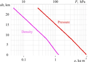
The profile of the atmospheric pressure measured during the bal-loonflight in March is identical to that recorded in February. The pressure varies exponentially with altitude with the characteristic heights of 7 and 6.2 km, respectively, below and above the altitude of ~8 km. The mass density of the N2‐dominated atmosphere
deduced from the measured temperature and pressure follows the same law as the gas pressure with the characteristic heights of 9 and 6.2 km, respectively, below and above the altitude of ~8 km. The variation of both parameters with height is displayed in Figure 5.
3.3. Geomagnetic and Weather Conditions
The global magnetic activity level was rather quiet during the February, 15flight and fairly high during March, 12 flight. Shown in Figure 6 are the variations of the north component of the mag-neticfield recorded by the Muonio (MUO) magnetometer of the northern Fennoscandia IMAGE network, situated close to the footprint of both balloon trajectories (Figure 3). Negative deviation in the north mag-netic component all along the March, 12flight corresponds to the substorm growth phase. Longitudinal distribution of the wide‐band photo emissions versus time is displayed at the same time scale as the mag-neticfield records. This keogram is produced from the ALFA all‐sky images (Section 2.3). Each column corresponds to a set of pixels along the line that connects the image center with the image east edge. Thus, assuming that the recorded photo‐emissions are mainly generated at the altitude of ~140 km, each column of the keogram corresponds to the longitude coverage of the all‐sky camera eastward from the ESRANGE.
In contrast with the March, 12, sky was covered with clouds and magnetic activity was low duringfirst two‐ thirds of the February, 15flight, but slightly increased after 21 UT. The SDA instrument operated until 20:46 UT during thisflight.
4. Observations
The method described in the Section 2.2 is used henceforth to correct the measured electric potentials, to cal-culate the vertical electricfield and the air electric conductivity.
4.1. Vertical Component of the Electric Field Versus Height Vertical component of the electricfield, Ev(in V m−1), was measured
during both ascent and descent phases of the February, 15 and March, 12 balloon flights. Its variation with height, z (in km), is shown in Figure 7 and is found to approximately follow the exponential function:
EVð Þ ¼ Ez 0⋅ exp −z=hð 0Þ: (4)
Both parameters, i.e. the characteristic height, h0, and amplitude, E0,
are height‐ dependent. Their amplitudes that provide the best fit to the measured series of data points are indicated in the Table 1. The change in the slope of the vertical electricfield observed during bothflights is related to the sharp variation of the horizontal wind at the altitudes of 15 and 10 km, respectively, for the February, 15 and March, 12 (see the right panel of Figure 7). The wind shear rate increases at these altitudes from ~0.7 10−3s−1to ~3–4 10−3s−1. In addition to the slope change, a slight shift in the measured electric field amplitude is seen in the ceiling and at ~15 km. This shift is caused by a quick variation of the balloon vertical speed.
Figure 4. Air temperature versus height for two balloonflights measured during
ascent (in magenta for 15.02.11 and in blue for 12.03.11) and descent (in red for 15.02.11 and in cyan for 12.03.11) phases.
Figure 5. Measured air pressure (in red) and deduced air mass density (in
magenta) versus height. The air pressure isfitted with: P(z)~ 1030e‐z/7below z = 8 km and P(z)~ 1160e‐z/6.2above z = 8 km. The air mass density isfitted with: ρ(z)~1.3e‐z/9below z = 8 km andρ(z)~2e‐z/6.2above z = 8 km.
Well above from the ground, the electricfield is produced by a misbalance between the ions of opposite polarities. The relationship between the elec-tricfield and the space charge density, ρ, is given by the Poisson equation, which in assumption that the main variations of the electrical parameters in atmosphere are vertical reads as:
dEV
dz ¼ ρ
ε0: (5)
According to (5), the positive space charge produces the positive deriva-tive of the vertical electricfield, like that measured during our balloon flights. Substituting the (4) in the (5), the variation of the space charge density versus height reads as:
ρ zð Þ ¼ −ε0E0
h0 ⋅ exp −z=hð 0Þ: (6)
The variation of this parameter with height is shown in Figure 8. Taking into account that the ion concentration in the low stratosphere is of order of 1010m−3and that the charge density at these heights is of order of 2⋅10−15C m−3(thus, of order of 104e m−3), one may conclude that only very insignificant fraction (~ 10−6for singled‐charged ions) of ions is not neutralised by the ions of opposite polarity. The discontinuity of the space charge density corresponding to the sharp change of the electricfield gradient is found at (or just above) the tropopause. Above this boundary, the number of the misbalanced charges is divided by three.
4.2. Electric Conductivity of Air Versus Height
The electric conductivity of air,σ (in S m−1), is a parameter which characterizes the capacity of light ions to carry the electric current in the atmosphere. This parameter is determined by the concentration of small‐ ions, ni(in m−1), their mobility,μ (in m2V−1s−1), and the electric charge carried by each ion, q (in C). It
reads as:
σ ¼ qμni: (7)
Even if this parameter was measured during entireflight, the most points depicted in the Figure 9 corre-spond to the observations performed in the stratosphere. The reasons of this are discussed in our previous paper [Seran et al., 2017] and are related to the limitations of the relaxation method. The method works well when the electricfield produced by the potential applied to the electrode in the initial phase of the relaxation Figure 6. Variations of north component of the magneticfield recorded by
MUO magnetometer during balloonflights on February, 15 (in magenta) and on March, 12 (in blue). Longitudinal distribution of light emission ver-sus time deduced from the ALFA all‐sky images is also displayed for March, 12flight. Balloon trajectory is depicted by white line.
Figure 7. Vertical component of the electricfield versus height, as measured during balloon flights on February, 15 (left)
and on March, 12 (centre). Measurements performed during the ascent and descent phases are shown in black and blue, respectively. Red lines correspond to the bestfit (4) with the parameters given in Table 1. Horizontal wind speed versus height, measured during February, 15 (mauve) and March 12 (blue)flights, are shown on the right panel.
10.1029/2018EA000463
Earth and Space Science
measurements is significantly higher than the ambient DC and AC (continuous and alternative) electricfield. This constraint does not create any problems for measurements made in the quiet Earth's stra-tosphere with electricfield of a fraction of V m−1, but it does if the instrument is used in lower atmosphere where the electric field exceeds ~few V m−1. With aim to extend the application domain of the instrument, a new design of the conductivity sensor was recently proposed and validated (see for the details Seran et al., 2017). In this design the sensitive part of the sensor is isolated from the external electricfield.
Similar to the electricfield, the electric conductivity of air varies exponentially with height, but its amplitude increases with altitude. The measured values are found to match:
σ±ð Þ ¼ σz 0⋅ exp z=hð 0Þ; (8)
withσ0≈ 2.3 10−13S m−1and h0= 7.8 km. The conductivities of both polarities are estimated to be close to
each other, with a minor surplus of ~2% for the negative conductivity. However, this excess is insignificant with respect to the mean absolute deviation of the measured points, which is ~8%.
Careful analysis of the air conductivity recorded during the March, 12flight indicates that the measured magnitudes are slightly less during balloon ascent than during its descent. This difference might be explained by a change of the auroral activity in time and with respect to the balloon location. During its ascent, the balloon crosses the edges of few thin isolated arcs (left keogram in Figure 9), i.e. eastward from the main region of the auroral emissions, while during its descent, the balloon moves through a diffuse part of the auroral oval (right keogram in the samefigure). Of course, the most energy of the energetic electrons precipitated during magnetic storms along the Earth magneticfield lines towards the atmosphere is lost in the ionosphere, i.e. at the altitudes between ~110 and 350 km. This energy goes to the ionisation of the atmo-spheric atoms and molecules, production of thermal electrons, generation of photo‐emissions. However, some part of very energetic electrons (with energies above few tens of keV) can reach the lower altitudes and contribute to the air ionisation. Even if the SDA data seems to give an indication in favour of such mechanism, the additional observations in conditions of stronger auroral activity have to be performed to approve or disapprove these observations.
The fact that the electricfield and electric conductivity profiles have the same characteristic height indicates that the density of the vertical electric current that circulates in the stratosphere is nearly constant and equals to
jvð Þ ¼ σz ð þþ σ−ÞEv≈3−4pAm−2: (9)
4.3. Lightning Detection in Stratosphere
Although in February–March the lightning activity attains its minimum in Europe, the lightning detection networks still record in average around few lightning strokes per minute. These strokes are mainly produced in the southern Europe, i.e. below ~45° geo lat (see, e.g. Anderson & Klugmann, 2014). The highest thunder-storm activity with, in average, one lightning per second is usually observed in July. Of cause, during thunderstorm periods, the light-ning rate is increased well above the above mentioned average values.
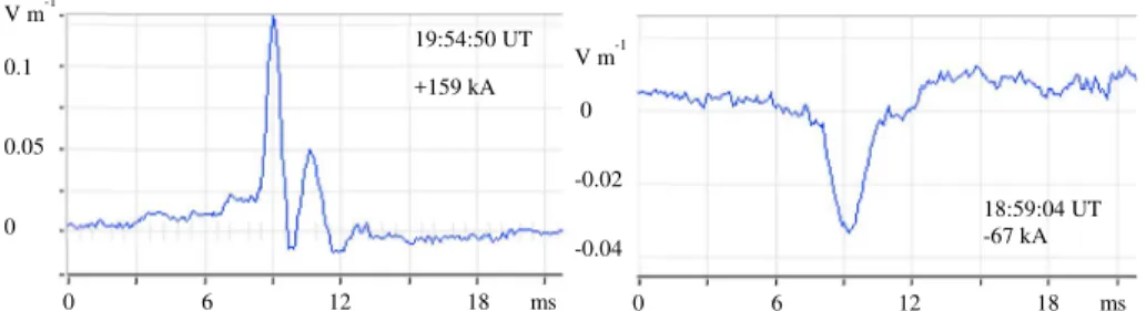
One example of the positive and negative lightning strokes detected simultaneousely by SDA and EUCLID network [see, e.g., Schulz et al., 2016] is presented in Figure 10. These two strokes with the peak currents, I, of +159 kA and− 67 kA induce the variation of the vertical electric field, Ev, of +130 mV
Table 1
Characteristic Parameters of the Vertical Electric Field Exponential Variation With Height
parameter
Februaryflight Marchflight ascent ascent descent ascent ascent descent 3 < z < 12.5 12.5 < z < 24 3 < z < 10 10 < z < 23
h0, km 2.9 7.8 7.8 2.6 7.8 7.8
E0, V m−1 −120 −5.6 −9 −140 −7 −10.5
Figure 8. Charge density versus height, as deduced from the electricfield
mea-sured during the balloonflights on February, 15 (magenta) and on March, 12 (blue). Small‐ion concentration is shown in red.
and − 33 mV at the distance, d, more than 3000 km from the source region. Comparing the measured amplitudes with those predicted by the transmission line model with Ev ~ 20 I/d (see,
e.g., Uman et al., 1975), one may conclude that only about 10% of the radiation field is transmitted at such distances. The rest is likely absorbed in the atmosphere or contributes to the excitation of waves in the extreme‐low frequency range (see, e.g., Price, 2016). With aim to demonstrate the relationship between the light-ning intensity and the Schumann resonances magnitudes, their temporal variations are shown in Figure 11 for the time period of 10 minutes starting from 21:28:21 UT on 12.03.11. The para-meters presented in this figure are deduced from the SDA mea-surements and consist of the total vertical electric field generated by the positive and negative lightningflashes each second together with the first and second harmonics of the Schumann resonance. The positive discharges, being in average two times less frequent with respect with the negative ones, are often associated with the stronger currents that generate the higher radiation fields. Increase of the electric field positive pulses above ~200 mV m−1 per second is observed to be related to an increase of the magni-tude of the second (~14.1 Hz) harmonic of the Schumann reso-nance above ~60 μV m−1.
5. Discussion
In this Section we use the measured data set to estimate some key parameters, such as mobility and concen-tration of small‐ions, their generation rate, as well as the radiation dose rate.
5.1. From Air Density to Small‐ion Mobility
The mobility of small‐ions is a parameter that is proportional to the ion charge and inversely propor-tional to the ion mass and collision frequency of the ion with other atmospheric species. Assuming that the effective mass and diameter of small ions do not change with the height, the mobility is estimated (see, for example, Bricard, 1965 or Wåhlin, 1994) to vary inversely with the air mass density, i.e.
μ±ð Þ≈z ρ0
ρ zð Þμ±0; (10)
hereμ±0≈ (1.6 ± 0.2)10−4m2V−1s−1at 0 °C and 103hPa. The negative ion mobility is quoted to be usually slightly higher than the positive one.
The air mass density, calculated in the Section 3.2.2 from the temperature and pressure measurements, is found to exponentially decrease with height as
Figure 9. Electric conductivity of air versus height, as measured during balloon
flight on March, 12. Solid and empty circles are used to show the measurements during the ascent and descent phases, respectively. Blue and red colours indicate the negative and positive ions conductivities, respectively. Longitudinal distri-butions of the of the wide‐band photo emissions versus time are displayed sepa-rately for the balloon ascent (on left) and descent (on right) phases. Balloon trajectory is indicated by white line.
Figure 10. Positive (left) and negative (right) cloud‐ground strokes detected by SDA at altitude of ~19.4 km on 15.02.2011.
Strokes were produced south‐west from the balloon location at the distance of ~ 3100 and 3200 km, respectively.
10.1029/2018EA000463
Earth and Space Science
ρ zð Þe1:3e‐z=9 below z¼ 8 km and ρ z
ð Þe2e‐z=6:2 above z¼ 8 km: (11)
Using (11), the (10) reads as
μ zð Þe1:5 10‐4ez=9 below z¼ 8 km and μ z
ð Þe10‐4ez=6:2 above z¼ 8 km: (12)
5.2. From Electric Conductivity of Air to Concentration of Small‐ions
Considering the measured values of the electric conductivity of air (8) and estimated values of the small‐ion mobility (12), the equation (7) at the altitudes above ~8 km reads as
nið Þ≈1:4⋅10z 10e‐z=31:5: (13)
The variation of the small‐ion concentration is displayed in Figure 8 together with the space charge density evaluated in Section 4.1.
5.3. Ion Generation Rate and Radiation Environment
One of the major sources of the atmospheric gas ionization in the Earth stratosphere is likely galactic cosmic rays and solar energetic particles. The radiation environment varies with the solar activity, geomagnetic lati-tude, solar zenith angle and atmospheric thickness (see, for example, Nehar, 1967; Reitz, 1993; Viggiano & Arnold, 1995; Singh et al., 2011). Usually the radiation level is measured in rad per time unit and is consid-ered to be one of the essential parameters for the preparation of space missions, definition of the protection level of space instruments and probability of their failure.
In our example and making some assumptions, the radiation dose rate can be roughly estimated from the deduced values of the ion density (13). Assuming for a simplicity that the ion recombination coefficient,
α, is constant and equals ~10−12m3s−1(see, for example, Cole & Pierce, 1965 or Shreve, 1970), the ion
pro-duction rate is estimated to be equal to
β zð Þ≈α⋅ni2ð Þ≈2⋅10z 8e‐z=16m‐3s‐1; 8<z<23 km: (14)
This expression is valid at the altitudes between 8 and 23 km, where we have an appropriate estimation of the ion density.
During its motion in a gas, each energetic particle undergoes numerous collisions with neutral species (molecules, atoms). These collisions result in a loss of their energy and in the generation of ions of both pola-rities. The radiation rate, B (in rad s−1), is related to the ion production rate, gas ionization energy, ei, and gas
mass density,ρ, as:
B≈β⋅ei
κρ ; (15)
Hereκ = 6.24 1016eV kg−1rad−1is conversion coefficient from rad to eV kg−1and the gas ionization energy Figure 11. Temporal variation of the total vertical electricfield generated by the positive (bleu) and negative (magenta)
lightningflashes each second together with the first (in red) and second (in black) harmonics of the Schumann reso-nance. The measurements are performed at the altitude of ~22 km during 10 minutes starting from 21:28:21 UT on 12.03.11.
is taken to be equal to ~35 eV. Substituting the previously estimated air mass density (Figure 5) and ion pro-duction rate (14) in the equation (15), the last reads:
B zð Þ≈5:6⋅10‐8ez=10rad s−1¼ 4:8⋅10‐3ez=10rad day−1; 8<z<23 km: (16)
Thus, one gets the radiation dose rate of 0.013 rad day−1at the altitude of 10 km and 0.035 rad day−1at 20 km.
6. Conclusions
We have presented the observations performed with the SDA instrument in the auroral atmosphere during two balloonflights in February and March of 2011. Two key parameters that characterize the electric proper-ties of the atmosphere were measured during theseflights, i.e. the electric field and the electric conductivity of air. The electricfield variation with the height was found to be controlled by the horizontal wind profile, while the temporal change of the electric conductivity of air was observed to correlate with the sub‐storm activity. Few parameters were deduced from the data measured during theflights, such as the charge den-sity, ion concentration, ion mobility and current density.
Lightningflashes produced in the southern Europe, i.e. more than ~ 3000 km from the balloon location, were clearly detected by the SDA AC channels. An increase of the positive strokes intensity above ~200 mV m−1s−1was shown to result in the amplification of the Schumann resonances amplitude up to ~ 150μV m−1.
The radiation dose rate that produces the air ionization in the lower stratosphere was estimated to vary between ~0.01 and 0.05 rad day−1. The radiation rate of ~0.018–0.026 rad day−1found between 13 and 17 km is comparable with that reported by Hassler et al. [2014] and measured on the Mars surface with the Radiation Assessment Detector (RAD) on the Mars Science Laboratory's Curiosity rover in 2012–2103.
References
Anderson, G., & Klugmann, D. (2014). A European lightning density analysis using 5 years of ATDnet data. Natural Hazards and Earth System Sciences, 14(4), 815–829. https://doi.org/10.5194/nhess‐14‐815‐2014
Balme, M., & Greeley, R. (2006). Dust devils on Earth and Mars. Reviews of Geophysics, 44, RG3003. https://doi.org/10.1029/2005RG000188 Bricard, J. (1965). Action of radioactivity and of the pollution upon parameters of atmospheric electricity, Problems of Atmospheric and Space
Electricity, (p. 82). Amsterdam: Elsevier Publ. Co.
Cole, R. K., & Pierce, E. T. (1965). Electrification in the Earth's atmosphere for altitudes between 0 and 100 kilometers. Journal of Geophysical Research, 70(12), 2735–2749. https://doi.org/10.1029/JZ070i012p02735
Farrell, W. M., & Desch, M. D. (2001). Is there a Martian atmosphere electric circuit? Journal of Geohysical Research, 106, 7591–7595. https://doi.org/10.1029/2000JE001271
Hassler, D. M., Zeitlin, C., Wimmer‐Schweingruber, R. F., Ehresmann, B., Rafkin, S., Eigenbrode, J. L., Brinza, D. E., et al. (2014). Mars's surface radiation environment measured with the Mars Science Laboratory's Curiosity Rover. Science, 343(6169), 1244797. https://doi. org/10.1126/science.1244797
Iles, R. H. A., Jones, J. B. L., Taylor, G. C., Blake, J. B., Bentley, R. D., Hunter, R., Harra, L. K., et al. (2004). Effect of solar energetic particle (SEP) events on the radiation exposure levels to aircraft passengers and crew: Case study of 14 July 2000 SEP event. Journal of Geophysical Research, 109, A11103. https://doi.org/10.1029/2003JA010343
Metzger, S.. (1999). Dust devils as Aeolian transport mechanisms in southern Nevada and Mars Pathfinder Landing Site. Ph.D. dissertation, University of Nevada, Reno.
Metzger, S. M., Balme, M. R., Towner, M. C., Bos, B. J., Ringrose, T. J., & Patel, M. R. (2011). In situ measurements of particle load and transport in dust devils. Icarus, 214(2), 766–772. https://doi.org/10.1016/j.icarus.2011.03.013
Molina‐Cuberos, G. J., Morente, J. A., Besser, B. P., Porti, J., Lichtenegger, H., Schwingenschuh, K., Salinas, A., et al. (2006). Schumann resonances as a tool to study the lower ionospheric structure of Mars. Radio Science, 41, RS1003. https://doi.org/10.1029/2004RS003187 Nehar, H. V. (1967). Cosmic rays particles that changed from 1954 to 1958 to 1965. Journal of Geophysical Research, 72, 1527–1539. https://
doi.org/10.1029/JZ072i005p01527
Price, C. (2016). ELF Electromagnetic Waves from Lightning: The Schumann Resonances. Atmosphere, 7(9), 116. https://doi.org/10.3390/ atmos7090116
Reitz, G. (1993). Radiation environment in the stratosphere. Radiation Environment in the Stratosphere, 48, 65–72. https://doi.org/10.1093/ oxfordjournals.rpd.a081837
Richon, P., Perrier, F., Sabroux, J.‐C., Trique, M., Ferry, C., Voisin, V., & Pili, E. (2005). Spatial and time variations of radon‐222 concen-tration in the atmospheres of a dead‐end horizontal tunnel. Journal of Environmental Radioactivity, 78(2), 179–198. https://doi.org/ 10.1016/j.jenvrad.2004.05.001
Schulz, W., Diendorfer, G., Pedeboy, S., & Poelman, D. R. (2016). The European lightning location system EUCLID– Part 1: Performance analysis and validation. Natural Hazards and Earth System Sciences, 16(2), 595–605. https://doi.org/10.5194/nhess‐16‐595‐2016 Seran, E., Godefroy, M., Kauristie, K., Cerisier, J.‐C., Berthelier, J.‐J., Lester, M., & Sarri, L.‐E. (2009). What can we learn from HF signal
scattered from a discrete arc. Annales de Geophysique, 27(5), 1887–1896. https://doi.org/10.5194/angeo‐27‐1887‐2009
10.1029/2018EA000463
Earth and Space Science
Acknowledgments
The SDA instrumental development and organization of the balloon campaign werefinancially supported by CNES Planetary and Balloon divisions. Special thanks to F. Vivat (LATMOS) who developed the software for SDA data acquisition. We thank the EUCLID network for the graceful provision of the lightning data. No other external data sets are used.
Seran, E., Godefroy, M., Pili, E., Michielsen, N., & Bondiguel, S. (2017). What can we learn from measurements of air electric conductivity in222Rn‐rich atmosphere. Earth and Space Science, 4, 91–106. https://doi.org/10.1002/2016EA000241
Seran, E., Godefroy, M., Renno, N., & Elliott, H. (2013). Variations of electricfield and electric resistivity of air caused by dust motion. JGR, Space Physics, 118(8), 5358–5368. https://doi.org/10.1002/jgra.50478
Shreve, E. L. (1970). Theoretical derivation of atmospheric ion concentrations, conductivity, space charge density, electricfield and gen-eration rate from 0 to 60 km. Journal of Atmospheric Sciences, 27(8), 1186–1194. https://doi.org/10.1175/1520‐0469(1970)027<1186: TDOAIC>2.0.CO;2
Singh, A. K., Siingh, D., & Singh, R. P. (2011). Impact of galactic cosmic rays on Earth's atmosphere and human health. Atmospheric Environment, 45(23), 3806–3818. https://doi.org/10.1016/j.atmosenv.2011.04.027
Uman, M. A., McLain, D. K., & Krider, E. P. (1975). American Journal of Physics, 43(1), 33–38. https://doi.org/10.1119/1.10027 Viggiano, A. A., & Arnold, F. (1995). Ion chemistry and ion composition, Handbook of atmospheric Electrodynamics, (Vol. 1). Boca Raton:
CRC Press.
Wåhlin, L. (1994). Elements of fair weather electricity. Journal of Geophysical Research, 99(D5), 10767–10,772. https://doi.org/10.1029/ 93JD03516