Distributed MAC protocol for networks with multipacket reception capability and spatially distributed nodes

Distributed MAC Protocol for Networks with Multipacket

Reception Capability and Spatially Distributed Nodes

by

Guner Dincer CELIK

Submitted to the Department of Electrical Engineering and Computer

Science

in partial fulfillment of the requirements for the degree of

Master of Science in Electrical Engineering and Computer Science

at the

MASSACHUSETTS INSTITUTE OF TECHNOLOGY

@

Massachusetts Institute

May 2007

of Technology 2007. All rights reserved.

Author

...

Department of Electrical Engineering and Computer Science

May 11, 2007

C

ertified by

...

_.r-v

...

_V...

_{. . ...}

Certified by

Eytan Modiano

A ... " ..

Accepted by..

AUG 16 2007

LIBRARIES

Thesis Supervisor

...

.

.. -

. ...

Arthur C. Smith

Chairman, Department Committee on Graduate Students

OCrVOf

Distributed MAC Protocol for Networks with Multipacket Reception

Capability and Spatially Distributed Nodes

by

Guner Dincer CELIK

Submitted to the Department of Electrical Engineering and Computer Science on May 11, 2007, in partial fulfillment of the

requirements for the degree of

Master of Science in Electrical Engineering and Computer Science

Abstract

The physical layer of future wireless networks will be based on novel radio technologies such as Ultra-Wideband (UWB) and Multiple-Input Multiple-Output (MIMO). One of the important capabilities of such technologies is the ability to capture a few packets simulta-neously. This capability has the potential to improve the performance of the MAC layer. However, we show that in networks with spatially distributed nodes, reusing MAC pro-tocols originally designed for narrow-band systems (e.g., CSMA/CA) is inefficient. It is well known that when networks with spatially distributed nodes operate with such MAC protocols, the channel may be captured by nodes that are near the destination. We show that when the physical layer enables multi-packet reception, the negative implications of reusing the legacy protocols include not only such unfairness but also a significant through-put reduction. We present a number of simple alternative backoff mechanisms that attempt to overcome the throughput reduction phenomenon. We evaluate the performance of these mechanisms via exact analysis, approximations, and simulation, thereby demonstrating that they usually outperform the legacy backoff mechanisms. We then discuss the implica-tions of the results on developing realistic MAC protocols for networks with a multi-packet reception capability and in particular for UWB networks.

Thesis Supervisor: Eytan Modiano Title: Associate Professor

Acknowledgments

I am profoundly thankful to my advisor, Prof. Eytan Modiano, and Post Doc. Assoc. Gil

Zussman for their support in this work, for their guidance that helped me continue my research in the right direction and for their friendly mood that makes it enjoyable to work with them.

I also would like to thank my family for their endless moral support throughout my career.

Finally, this work was supported in part by ONR under grant N000140610064, and by a grant from Draper Laboratory.

Contents

1 Introduction 17

2 Related Work 23

3 System Description and Assumptions 29

3.1 Backward Protocol ... 32

4 Examples 33 4.1 Aloha with Two Distances: Example 1 ... . 33

4.2 Aloha with Two Distances: Example 2 ... 36

4.3 Backward Protocol with Random Distances and Single Capture: Example 3 37 5 Protocol Analysis 41 5.1 Random Locations Without Fading ... ... . . 41

5.2 Deterministic Locations -Without Fading . ... 46

5.2.1 Exact Model With Nodes at One of Two Different Locations . . . . 46

5.2.2 Basic Approximate Model ... ... 61

5.2.3 Enhanced Approximate Model ... . 65

5.3 Deterministic Locations-With Fading ... .. 79

5.4 Random Locations With Fading ... 82

5.4.1 Approximating pc(r) Using -(r). .... ... 83

5.4.2 Approximating pc(r) Using Jensen's Inequality ... 85

6.1 Backward Model with Forced Idle Periods . ... 90

6.2 Backward Model with Dynamic Contention Windows ... 94

7 Performance Evaluation and Simulations 97 7.1 Deterministic Locations Without Fading . ... 98

7.2 Random Locations Without Fading ... ... 102

7.3 Random Locations With Fading Simulation . ... . 103

7.4 Backward Model with Forced Idle Periods . ... 107

7.5 Backward Model with Dynamic Contention Windows ... 108

8 Conclusion and Future Work 115

A Analytical solution of (4.3) and (4.4) in the case of two nodes 117 B The Transition Probabilities of The 1-Dimensional Markov Chain of Section

5.2.1 119

List of Figures

1-1 An example scenario where 1 nearby node captures the channel (since its signal is greater) and blocks 4 faraway nodes. The transmitting nodes are indicated with arrows. This is a very inefficient use of the network resources if the maximum number of simultaneously received transmissions in the network is greater than 1, i.e., if the receiver is capable of

receiving multiple packets at a time. . ... ... 18

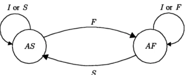
3-1 The Single User State Diagram, S: Success, 1: Idle, F: Failure, AS: After Success, AF: After Failure. ... 32

4-1 Simple spatial distribution. ... 34

4-2 Throughput plot for the system in Example-1 for nl = 1, n2 = 3 and z = 0.2... 36

4-3 Throughput plot for the system in Example-2 for nl = 2 ,n2 = 6 and z = 0.2... . 37

4-4 The transmission probability and the throughput as a function of distance under the for-ward (Pt, = 0.2 and Ptf = 0.05) and the backward (pt, = 0.05 and Ptf = 0.2.) backoff mechanisms for a = 2 and uniform distribution of 12 nodes on a disk. . ... 39

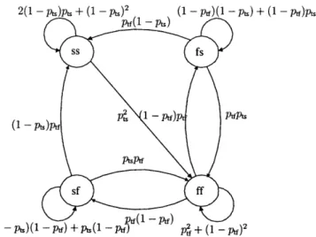
5-1 System Markov Chain in Example-2, Case-a. ss: both nodes are successful, sf: node-i is successful and node-2 is failed in its last attempt. . ... 43

5-2 System Markov Chain in Example-2, Case-b. ... ... . . . 43

5-3 The comparison of the transmission probability and the throughput of the exact and the approximate analysis for a = 2, Pts = 0.2 and Pt$ = 0.05 (i.e., for the forward model case) and uniform distribution of 2 nodes on a disk ... 46

5-4 The Markov Chain for the analysis in Section 5.2.1 for nl = 6, n2 = 10 and z = 0.2. Note that only some of the transition probabilities of the state (nl, n2) = (4, 6) are shown. 48

5-5 Throughput plot for deterministic locations case with rl = 1, r2 = 2, nl = 1, nz2 = 5 and

z = 0.2 . . . .

5-6 Throughput of the faraway nodes for deterministic locations case with ri

n = 1, n2 = 5 andz = 0.2. ...

5-7 Throughput plot for deterministic locations case with r1 = 1, r2 = 2, nl

andz = 0.2 .. . . . ..

5-8 Throughput of the faraway nodes for nl = 2, n2 = 10 and z = 0.2 . . .

5-9 Throughput plot for deterministic locations case with ri = 1, r2 = 2, nl -andz= 0.2 . . . . 5-10 Throughput of the faraway nodes for deterministic locations case with rl

nl = 6, n2= 10 and z = 0.2. ... =1, = 2, 6, =1, =2, S10 =10 =2,

5-11 Throughput plot for nl = 1, n2 = 5 and z = 0.2 using the Basic Approximate Model.. 5-12 Throughput plot for deterministic locations case with rl

and z = 0.2 using the Basic Approximate Model. . . 5-13 Throughput plot for deterministic locations case with rl

and z = 0.2 using the Basic Approximate Model. 5-14 Network Structure, Enhanced Approximate Model. 5-15 Throughput plot for deterministic locations case with rl

z = 0.2 using the Enhanced Approximate Model. . . 5-16 Throughput plot for deterministic locations case with rl

and z = 0.2 using the Enhanced Approximate Model. . 5-17 Throughput plot for deterministic locations case with rl

and z = 0.2 using the Enhanced Approximate Model. .

= 1, r2 = 2, ni = 1, r2 = 2, nl = 2, n2 = 6, n2 = 1, r2 = 2, ni = 1, n2 = . 1, . = 2, n = 2., n2 = 1, r2 = 2, nl = 6, n2 . . . . . . . . . . . .

5-18 Throughput plot for deterministic locations case with rl = 1, r2 = 2, r3 = 4, ni = 1,

n2 = 2, n3 = 4 and z = 0.2 using the Enhanced Approximate Model . . . . .

5-19 Throughput plot of the users at distance 2 for deterministic locations case with r1 = 1,

r2 = 2, r3 = 4, nl = 1, n2 = 2, n3 = 4 and z = 0.2 using the Enhanced Approximate

M odel . . . .... 10 =10 = 10 5 and = 10 = 10

5-20 Throughput plot of the users at distance 4 for deterministic locations case with ri = 1, r2 = 2, r3 = 4, ni = 1, n2 = 2, ns = 4 and z = 0.2 using the Enhanced Approximate

Model ... ... 77

5-21 Throughput plot for the case of deterministic locations with fading in the channel. The number of nodes at distances rl = 1, r₂ = 2 and r3 = 3 are nl = 1, n2 = 3, n3 = 9 respectively, and z = 0.2. ... 82

5-22 Throughput plot for random node locations case with fading in the channel for n = 10 and z = 0.2 using the Jensen's Inequality approximation to the average of Pc,k(r) ... 84

5-23 The upper and lower bounds to Pc,k(r) as a function of distance, r for n = 10 nodes in

the system and z = 0.2. The figure corresponds to k = 5 ... 86

5-24 Throughput plot for random node locations case with fading in the channel for n = 10

and z = 0.2 using the Jensen's Inequality approximation to the average of pc,k (r) ... 87

6-1 Throughput plot for deterministic locations case (no fading) with r1 = 1, r2 = 2, ni = 5,

n2 = 15 and z = 0.2 using the original model. . ... . 91

6-2 Throughput plot of the users at distance 1 for deterministic locations case (no fading) with

rl = 1, r2 = 2, nl = 5, n2 = 15 and z = 0.2 using the original model. . ... 91

6-3 Throughput plot of the users at distance 2 for deterministic locations case (no fading) with

ri = 1, r2 = 2, ni = 5, n2 = 15 and z = 0.2 using the original model. . ... 91

6-4 The single user state diagram for the Backward Model with Forced Idle Periods. This figure corresponds to having nodes stay idle for 1 slot after a successful transmission. S: Success, I: Idle, F: Failure, WAS: Wait After Success, AF: After Failure, TAW: Transmit After Waiting. The transition labeled by "a" occurs with probability 1. . ... 92

7-1 Comparison of the total network throughput in the simulation model and in the exact model for deterministic node locations and without fading in the channel where TP-Sim stands for throughput obtained by simulation and TP-Exact that from the exact analysis. We utilized nl = 1, n2= 5, rl = 1, r2= 2, z = 0.2 and t = 100K. . ... . 98

7-2 Comparison of the aggregate throughput of the distance-2 users in the simulation model and in the exact model for deterministic node locations and without fading in the channel where TP-Sim stands for throughput obtained by simulation and TP-Exact that from the exact analysis. We utilized nl = 1, n2 = 5, r1 = 1, r2 = 2, z = 0.2 and t = 100K. . . . 99

7-3 Comparison of the total network throughput in the simulation model and in the exact model for deterministic node locations and without fading in the channel where TP-Sim stands for throughput obtained by simulation and TP-Exact that from the exact analysis. We utilized nl = 1, n2 = 5, rl = 1, r2 = 2, z = 0.2 and t = 1000k. . ... 99

7-4 Comparison of the aggregate throughput of the distance-2 users in the simulation model and in the exact model for deterministic node locations and without fading in the channel where TP-Sim stands for throughput obtained by simulation and TP-Exact that from the exact analysis. We utilized ni = 1, n2 = 5, r, = 1, r2 = 2, z = 0.2 and t = 1000k. . . . 99

7-5 Comparison of the total network throughput in the simulation model and in the exact model for deterministic node locations and without fading in the channel where TP-Sim stands for throughput obtained by simulation and TP-Exact that from the exact analysis. We utilized nl = 2, n2 = 10, rl = 1, r2 = 2, z = 0.2 and t = 100K. ... 100

7-6 Comparison of the total network throughput in the simulation model and in Enhanced Approximate Model for deterministic node locations and without fading in the channel where TP-Sim stands for throughput obtained by simulation and TP-App. that from the approximate model. We utilized nl = 1, n2 = 2, n3 = 4, rl = 1, r2 = 2, r3 = 4,

z=0.2andt=100K ... ... 101

7-7 Comparison of the aggregate throughput of the distance-2 users in the simulation model and in Enhanced Approximate Model for deterministic node locations and without fading in the channel where TP-Sim stands for throughput obtained by simulation and TP-App. that from the approximate model. We utilized n, = 1, n2 = 2, n3 = 4, rl = 1, r2 = 2,

7-8 Comparison of the aggregate throughput of the distance 4 users in the simulation model and in Enhanced Approximate Model for deterministic node locations and without fading in the channel where TP-Sim stands for throughput obtained by simulation and TP-App. that from the approximate model. We utilized nl = 1, n2 = 2, n3 = 4, rl = 1, r2 = 2,

r3 = 4, z = 0.2 and t = 100K. ... 101

7-9 Total network throughput when there are 10 uniformly distributed nodes on a plane (no fading) with z = 0.2, t = 100K and 40 iterations. . ... . 102 7-10 Total network throughput when there are 20 uniformly distributed nodes on a plane (no

fading) with z = 0.2, t = 100K and 40 iterations. . ... . 102 7-11 Total network throughput when there are 40 uniformly distributed nodes on a plane (no

fading) with z = 0.2, t = 100K and 40 iterations. . ... . 103

7-12 Total network throughput when there are 10 uniformly distributed nodes on a disk with fading in the system for z = 0.2, t = 100K and 40 iterations. . ... . 104 7-13 Total network throughput when there are 20 uniformly distributed nodes on a disk with

fading in the system for z = 0.2, t = 100K and 40 iterations . ... 104 7-14 Total network throughput when there are 50 uniformly distributed nodes on a disk with

fading in the system for z = 0.2, t = 100K and 40 iterations. . ... . 104 7-15 Total network throughput when there are 100 uniformly distributed nodes on a disk with

fading in the system for z = 0.2, t = 100K and 40 iterations. . ... . 105

7-16 Total network throughput when there are 10 uniformly distributed nodes on a disk with fading in the system for z = 0.1, t = 100K and 40 iterations. . ... . 106

7-17 Total network throughput when there are 10 uniformly distributed nodes on a disk with fading in the system for z = 0.3, t = 100K and 40 iterations. . ... . 106

7-18 Total network throughput when there are 10 uniformly distributed nodes on a disk with fading in the system for z = 0.5, t = 100K and 40 iterations . ... 106

7-19 Total network throughput when there are 10 uniformly distributed nodes on a disk with fading in the system for z = 0.7, t = 100K and 40 iterations. . ... . 107

7-20 Total network throughput of the Backward Model with Forced Idle Periods for ri = 1,

r2 = 2, ni = 5, n2 = 15, z = 0.2 and t = 100K in the case where nodes stay idle for 2 slots after each successful transmission. . ... .... 108

7-21 Throughput of the nodes at distance 1 for Backward Model with Forced Idle Periods for

rl = 1, r2 = 2, ni = 5, n2 = 15, z = 0.2 and t = 100K in the case where nodes stay

idle for 2 slots after each successful transmission. . ... 108 7-22 Throughput of the nodes at distance 2 for Backward Model with Forced Idle Periods for

rl = 1, r2 = 2, nl = 5, n2 = 15, z = 0.2 and t = 100K in the case where nodes stay

idle for 2 slots after each successful transmission. ... .... 109

7-23 Total network throughput of the Backward Model with Forced Idle Periods for rl = 1,

r2 = 2, nl = 5, n2 = 15, z = 0.2 and t = 100K in the case where nodes stay idle for 8 slots after each successful transmission. . ... .... 109

7-24 Throughput of the nodes at distance 1 for Backward Model with Forced Idle Periods for

rx = 1, r2 = 2, n1 = 5, n2 = 15, z = 0.2 and t = 100K in the case where nodes stay

idle for 8 slots after each successful transmission. . ... 109

7-25 Throughput of the nodes at distance 2 for Backward Model with Forced Idle Periods for

rl = 1, r2 = 2, n1 = 5, n2 = 15, z = 0.2 and t = 100K in the case where nodes stay

idle for 8 slots after each successful transmission. . ... . . 110

7-26 Total network throughput for Backward Model with Dynamic Contention Windows for

r, = 1, r2 = 2, nl = 1, n2 = 5, z = 0.2 and t = 100K. ... 110 7-27 Total throughput of the nodes at distance 1 for Backward Model with Dynamic Contention

Windows for rl = 1, r2 = 2, nl = 1, n2 = 5, z = 0.2 and t = 100K. . ... 111 7-28 Total throughput of the nodes at distance 2 for Backward Model with Dynamic Contention

Windows for rl = 1, r 2 = 2, nl = 1, n2 = 5, z = 0.2 and t = 100K. . ... 111

7-29 Total network throughput of the Backward Model with Dynamic Contention Windows for

rl = 1, r2 = 2, n1 = 2,n2 = 10, z = 0.2 andt = 100K ... 112

7-30 Total throughput of the nodes at distance 1 for Backward Model with Dynamic Contention

Windows for r, = 1, r2 = 2, ni = 2, n2 = 10, z = 0.2 and t = 100K. ... 112

7-31 Total throughput of the nodes at distance 2 for Backward Model with Dynamic Contention

Windows for r = 1, r2 = 2, nl = 2, n2 = 10, z = 0.2 and t = 100K. ... 113 7-32 Total network throughput of the Backward Model with Dynamic Contention Windows for

ri = 1, r2 = 2, r3 = 3, ni = 1, n2 = 3, n3 = 9, z = 0.2 and t = 100K. . ... 113

7-33 Throughput of the node at distance 1 for Backward Model with Dynamic Contention

Win-dows for ri = 1, r2 = 2, ra = 3, n, = 1, n2 = 3, n3 = 9, z = 0.2 and t = 100K. .... 113

7-34 The aggregate throughput of the nodes at distance 2 for Backward Model with Dynamic

Contention Windows for rl = 1, r2 = 2, r3 = 3, nl = 1, n2 = 3, n3 = 9, z = 0.2 and

t= 100K ... ... 114

7-35 The aggregate throughput of the nodes at distance 3 for Backward Model with Dynamic

Contention Windows for rl = 1, r2 = 2, r3 = 3, nl = 1, n2 = 3, n3 = 9, z = 0.2 and

t= 100K .. . . . 114

A-i The transmission probability obtained analytically and numerically as a function of dis-tance for pt = 0.2, ptf = 0.05, a = 1 and uniform distribution of 2 nodes on a line. . . . 118

Chapter 1

Introduction

Future communication technologies such as UWB, MIMO or existing spread spectrum sys-tems such as code division multiple access (CDMA) have fundamental differences from the corresponding narrowband or single antenna systems. Although some medium-access con-trol (MAC) protocols for UWB have been proposed [3,10,14,20,26,39], they do not take into account the special characteristics of the system such as multipacket reception capa-bility. In this thesis we focus on fundamental aspects of MAC layer design for multipacket reception networks with spatially distributed nodes.

In wideband communications the information is spread over a very wide bandwidth using time hopping or spreading codes at the transmitter [57]. In a packet based network, this spreading enables the receiver to demodulate multiple packets at a time. The same result is observed in MIMO systems by the use of multiple antennas at the receiver. This capability of multipacket reception introduces new challenges in designing MAC protocols [18,59].

The basic underlying assumption in legacy MAC protocols (e.g., slotted aloha) is that any concurrent transmission of two or more users causes all transmitted packets to be lost [5]. However, this model does not reflect the actual situation in many practical wireless networks where some information can be received correctly from a simultaneous transmis-sion of several packets. Therefore, this assumption has been subjected to some improve-ments in literature. The first improvement is called the capture effect: The packet with the strongest power level can be received successfully (captured) in the presence of

con-Figure 1-1: An example scenario where 1 nearby node captures the channel (since its signal is greater) and blocks 4 faraway nodes. The transmitting nodes are indicated with arrows. This is a very inefficient use of the network resources if the maximum number of simultaneously received transmissions in the network is

greater than 1, i.e., if the receiver is capable of receiving multiple packets at a time.

tending transmissions if its power level is sufficiently high. It occurs in networks with single packet reception capability where packets arrive at the common receiver with dif-ferent power levels due to near-far effect, shadowing or fading. The effect of capture on Aloha [1, 2, 27, 28, 30, 51, 52, 62] and on IEEE 802.11 protocol (Carrier Sense Multiple Access-Collision Avoidance (CSMA/CA)) [23,24,36, 43] has been studied extensively in the literature and new MAC protocols for channels with capture have been proposed [11]. Hajek et al. [25] provided asymptotic results on the capture probability in the limit of in-finite number of users. The other major improvement to the original model, known as multipacket reception capability, assumes that a subset of the collided packets can be re-ceived successfully. The impact of the multipacket reception capability on MAC protocols has received limited attention to date. Ghez et al. [18, 19) proposed a channel model for networks with multipcaket reception capability and studied stability properties of slotted aloha in such a setting. Peh et al. [44] revisited the model of [18] and proposed improve-ments in retransmission control schemes by utilizing additional feedback. Tong et al. have proposed MAC protocols based on multipacket reception capability [37, 38, 59, 60] using the channel model suggested in [18]. The protocols developed in [59, 60] maximize the per-slot throughput by controlling the set of users who are allowed to transmit in each slot. However, these protocols require a centralized controller and hence are impractical for large distributed networks. Nguyen et al. [42] considered the SNR model for capture and derived expressions for capture probability for both narrowband (single capture) and wideband (multiple packet reception) communication systems. Furthermore, new MAC algorithms for multipacket reception channels were proposed in [7,31,47,48].

Note that there are other solutions rather than designing a MAC protocol specific to this setting, yet each of them has its own disadvantages. First, using power control schemes where nodes are allowed to choose the power level with which to send their packets has been proposed in [29,33,40,52] for the single capture case and in [34] for the multipacket reception case. However, power control mechanisms require sophisticated feedback and complex transmitters that can adjust the transmit power level dynamically. Hence expen-sive transmitters are needed which might be a problem for networks with large number of nodes. Moreover, for more realistic network settings such as multi-hop networks with many receivers, every node can send to a subset of the receivers and adjusting the power level according to different feedback from different receivers makes the design more com-plicated. A second alternative is to use Time Division Multiple Access (TDMA) technique. Applying TDMA schemes directly to multipacket reception channel not only causes exces-sive delays but also results in very inefficient usage of channel resources since the receiver can capture multiple packets at a time, hence allowing some contention is in fact preferred. Optimal scheduling algorithms for TDMA networks with multipacket reception capability have been studied in [9,53], however, they require a centralized controller together with an advanced feedback mechanism making it difficult to utilize them in large network settings such as multihop networks.

Multipacket reception capability in networks with spatially distributed nodes calls for new MAC protocols as well. However, previous work in this field mostly do not take into account the spatial distribution of the nodes, which, as we explain shortly, results in very inefficient utilization of the channel and unfairness when existing MAC protocols are used in this network setting. It is well-known that existing MAC protocols (e.g., IEEE 802.11) are unfair and may starve some of the nodes [4, 6, 16,55]. The reason for this is that if a node has a successful transmission, IEEE 802.11 gives a higher transmission probability to that node and a lower probability to the failed node. Consequently, successful users con-tinue to capture the channel and the failed users concon-tinue to transmit with low probability, resulting in starvation of some of the nodes in the network. This fairness phenomenon is even more pronounced in networks with spatially distributed nodes since the distant users have weaker signals than nearby users due to the severe attenuation of the signal power with

distance. Consequently, packets belonging to distant users are lost with higher probabil-ity. Futhermore, when there is multipacket reception capability in a network with spatially distributed nodes, unfairness amounts to very inefficient usage of the channel resources. For example consider that an IEEE 802.11 type protocol is applied to such a network and consider the collision of a nearby user and 4 distant users as shown in Fig. 1-1. In a typi-cal scenario, the packet of the nearby node is received successfully and the others are lost since the power level of the nearby user is much greater than that of the distant users. Once the faraway node senses the collision, it increases its contention window (i.e., decreases its transmission probability) and the successful nearby node decreases its contention window (increases its transmission probability) continuing to capture the channel. Thus even the less frequent transmissions of the remote users will be unsuccessful leading to their com-plete starvation. This means that, one user might dominate the network and starve several distant users. Hence unfairness in multipacket reception channels with spatially distributed nodes may lead to very low overall network throughput. The above example suggests that a fair protocol in such a network should give a greater chance to distant users in order to prevent their starvation in the network. Moreover, under most spatial distributions the num-ber of remote nodes is considerably greater than that of nearby nodes and hence allowing a higher transmission probability to distant users can increase the network throughput. This is the main idea of this work where we design and analyze a distributed MAC protocol for networks with multipacket reception capability and spatially distributed nodes. Our pro-tocol is simple to operate and easy to extend to more complicated network structures. We start with a single receiver, single hop system in this thesis, however, ultimately we aim at extending this protocol to multi-hop settings.

A simple alternative scheme to what has been done in CSMA/CA type traditional algo-rithms would have the node use a high transmission probability following a collision and a low transmission probability following a success. This simple scheme will be referred to as the backward model. We propose the Backward Protocol inspired by this idea and show by some motivating examples in Chapter 4, that the Backward Protocol gives greater chances to distant nodes and achieves better performance than the traditional mechanisms which employ the forward model (i.e., having large transmission probability after a success

and a low transmission probability after a failure).

We develop comprehensive analysis of the protocol in various settings. We start with an analysis of the case where the nodes are randomly distributed on a plane without fading in the channel. Next, we analyze the protocol when the node locations are deterministic and there is no fading in the channel. We give exact analysis together with approximations that enable us to extend the results to more sophisticated networks (i.e., more allowed distances from the receiver and more users) with high accuracy. We utilize approximation techniques to analyze the cases where there is multipath fading in the channel both when the node locations are deterministic and when they are random. We show by numerical analysis that the Backward Protocol gives more fair results in all of the cases and better throughput results in most of the cases described above.

In addition to the exact and the approximate analysis of the protocol under different scenarios, we provide simulation results for the network settings where the approximate models no longer hold and we compare the effect of different parameters in the model. Finally, based on the results obtained from these simple mechanisms, we attempt at de-veloping more realistic MAC protocols for networks with multipacket reception capability and spatially distributed nodes.

The main contributions of our work are the following. We propose the Backward Pro-tocol that is a dynamic MAC proPro-tocol designed for networks with multipacket reception capability and spatially distributed nodes. We show by analysis and simulations that the Backward Protocol deals with the severe fairness problem due to the near-far effect and it achieves higher throughput values than traditional back-off mechanisms in most cases considered. Finally, we provide various approximations that are accurate and useful in

analyzing the performance of the network for more complicated settings.

The organization of the thesis is as follows. We begin with the previous work in this field and describe what has been done in literature in a similar context in Chapter 2. In Chapter 3, we give the system description and assumptions used for the channel, the feed-back, and the users. We also describe the Backward Protocol in a detailed manner in this chapter. In Chapter 4, we give some motivating examples which suggest that the proposed scheme functions better than existing MAC protocols in terms of throughput and fairness.

In Chapter 5, we analyze the proposed protocol in various different settings. In Chapter 6 two new protocols which are improved versions of the original protocol are considered. Finally, extensive simulation results are presented in Chapter 7.

Chapter 2

Related Work

The related work regarding the effect of capture on MAC protocols starts with the work of Roberts [49] who introduced the so called perfect capture model as the packet of the user with the largest received power is correctly demodulated out of a collision of many packets. He also suggested the vulnerability circle model for capture which assumes that a packet transmitted from distance r is successfully received if no other packet is gen-erated within a circle of radius ar. Metzner [40] studied the perfect capture model for Aloha protocol with power control and computed the optimal probabilities (optimal in the sense that it maximizes the throughput) with which transmitters should use the available power levels. Abramson analyzed the Aloha protocol under vulnerability circle model in [1] and Shacham [52] studied perfect capture model in Aloha protocol with multiple transmit power levels. Kuperus and Arnbak [28] considered the SNR model for capture and termed it capture ratio, which assumes that a packet is correctly received if its received power exceeds the total interference power by more than a threshold factor z (hence the name SNR model), and derived probability of capture in a channel with Rayleigh fading. Arnbak and Van Blitterswijk [2] extended the results in [28] for a channel with combined near-far effect and Rayleigh fading. Cidon, Kodesh and Sidi [11] introduced and analyzed different MAC protocols to exploit the capture effect and discussed the power control idea in such a setting. Lau and Leung [30] considered various spatial distributions and provided a comparison of the vulnerability circle and the SNR models. A more detailed review of the work in this field until 1993 can be found in Linnartz's book [32], where he also analyzed

many cases for the SNR model.

Then the subsequent works of Zorzi and Rao [62], and Krishna and Lamaire [27] ex-tended the results in [32] about MAC protocols with capture and derived expressions for the capture probability when there are n contending transmissions, C,, using the SNR model. Moreover, Zorzi and Rao [62] provided stability results for ALOHA protocol with capture, which states that the protocol is stable if the arrival rate to the system, A is less than C, where C, is the capture probability in the limit of infinitely many transmissions. They also proposed a retransmission control scheme to stabilize unstable systems. Some corrections to this work was suggested in [41], followed by the reply [63]. As mentioned in the previ-ous section, Lamaire, Krishna, and Zorzi in [29] and Luo and Ephremides in [33] proposed a power control scheme for networks with capture, where the nodes have discrete trans-mit power levels. LaMaire et al. [29] determined the optimal transmit probabilities for the

power levels together with the optimal values of the power levels themselves for maximiz-ing the capture probabilities. Luo and Ephremides [33] showed that the smaximiz-ingle power level system achieves optimal throughput when some decodability threshold value (i.e., SNR of each packet is above a certain level) for received packets is satisfied. Zorzi [61] extended the throughput analysis in [62] to the case where there is diversity, Rayleigh fading and shadowing in the system. Finally, Sant and Sharma [51] analyzed stability properties of slotted aloha from queuing theory perspective when there is capture effect and fading in the system.

Bianchi [17] analyzed IEEE 802.11 (CSMA/CA) protocol with finite number of users assumption. Hadzi-Velkov and Spasenovski [22-24] extended [17] to the case where there is capture in the channel under various settings (with and without Rayleigh fading and diversity in the channel). Manshaei et al. [36] extended the previous results on IEEE 802.11 with capture to the case where the nodes have different distances in the network. Nyandoro

et al. [43] analyzed IEEE 802.11 protocol with capture and showed that the probability

of successful reception increases when nodes use one of the two different power levels according to their service class. As pointed out in the introduction, there are many work on fairness and throughput starvation in IEEE 802.11 (CSMA/CA) type protocols [4,6,16,55], however, they are not aimed at multipacket reception channels and the fairness issue due to

the near-far effect is not addressed in most of them.

Ghez et al. studied the effect of multi-packet reception on Aloha protocol in [18] where they generalized the collision channel model by modeling the number of successfully re-ceived packets in each slot as a random variable which depends only on the number of transmissions on that slot. They derived the maximum stable throughput of Aloha channel under these assumptions. They extended the analysis, provided stability results also for the case in which the retransmission probabilities can be varied as a function of the channel history and presented a protocol that stabilizes the general system in [19]. Peh et al. [44] revisited the model of [18] and proposed improvements in retransmission control schemes by utilizing additional feedback. Tong et al. [37, 38, 56, 59, 60] used the model of [18] and extended the analysis in various directions. In particular, Zhao and Tong [59, 60] designed new MAC protocols based on multipacket reception capability that maximizes the expected number of successfully received packets per slot by controlling the set of users who are al-lowed to transmit in each slot depending on the channel history and the QoS constraints of the users. Hajek et al. [25] provided asymptotic results on the capture probability in the limit of infinite number of users. Chan and Berger [8] analyzed an extension of CSMA protocol (assuming nodes can sense the power level in the channel and hence the number of packets currently being transmitted) in multipacket reception networks using the chan-nel model suggested in [18]. Likhanov et al. [31] presented and analyzed new algorithms for multipacket reception networks based on collision resolution technique. Yu et al. [58] provided conditions on spatial distribution function of nodes for stability of Aloha protocol in multipacket reception channel. Nguyen et al. [42] considered the SNR model for capture and derived expressions for capture probability for both narrowband (single capture) and wideband (multiple packet reception) communication systems.

Different approaches to the multi-access control in multipacket reception networks in-clude a cross layer design protocol in [47] by exchanging parameters between physical and MAC layer. A similar approach was studied in [48] for the MIMO multiple access channel both from physical layer and MAC layer perspectives giving formulations for a cross layer optimization to maximize throughput. A MAC protocol for a spread spectrum multihop network which dynamically adjusts its behavior according to channel feedback

was described in [7]. Luo and Ephremides extended [33] to multipacket reception net-works [34] and showed that the single-power-level-system achieves optimal throughput if SNR levels of packets are above some threshold. Extensions of TDMA type schemes to multipacket reception channels have been proposed, e.g., in [9] optimal scheduling (for maximum throughput) of transmissions on multiple independent channels is studied. A dynamic slot allocation scheme in multipacket reception channel using antenna arrays is proposed in [53]. Coupechoux et al. [13] analyzed the performance of slotted aloha on multihop multipacket reception network setting as well as discussing new issues on the de-sign of MAC layer in such a setting [12]. Finally, Mackenzie and Wicker [35] presented a game theoretic analysis of the model of Ghez et al.

Moreover, recently there has been some interest [15] in UWB MAC layer which aims to address specific properties of the UWB physical layer suggested in [57]. Optimal schedul-ing and routschedul-ing problems in UWB physical layer are studied in [46, 54]. Radunovic and Boudec [45] showed that due to the distinct characteristics of UWB-Impuls Radio (UWB-IR), reusing medium access control (MAC) protocols originally designed for narrow-band systems may be inefficient. A few aspects of the UWB MAC layer have been been studied in for example [3,39]. In [10, 14,20,26] optimization problems that attempt to address the particular properties of the physical layer are formulated and the results of these optimiza-tions are used as a basis for a MAC protocol design.

These previous work specific to UWB is different from what is in this thesis in that they are explicitly based on UWB physical layer whereas we propose a more general MAC pro-tocol that can work on all multipacket reception channels with spatially distributed nodes (e.g., CDMA, UWB etc.). Furthermore, we study the problem from a more fundamen-tal point of view and obtain analytical results while the above mentioned works mostly evaluate the performance of some heuristic idea using simulations.

Furthermore, most of the above previous work on MAC layer design for general multi-packet reception channels did not assume a spatial distribution of the nodes on the network. In the cases where a spatial distribution was considered, the throughput reduction due to near far effect and the starvation of distant nodes were not taken into account. Furthermore, in most cases the effect of capture or the multipacket reception capability on the existing

MAC protocols (Aloha mostly) were studied. The new protocols suggested for multipacket reception channel required a centralized controller and sophisticated feedback mechanisms making the protocol computationally complex and impractical for distributed networks. However a new MAC protocol design that will exploit the multipacket reception capability and remedy the fairness problem when the nodes are spatially distributed is necessary and this is the topic of this thesis.

Chapter 3

System Description and Assumptions

Consider a system where users are communicating to a receiver with possibly different dis-tances from it. The receiver can be a base station as in cellular networks or an access point as in multi-hop wireless networks. We assume single destination, single-hop system in this thesis, however, our ultimate objective is to extend the protocol to multi-hop networks. Therefore, we assume the receiver does not control the transmissions of the users and we design a distributed protocol which will be explained in details shortly. We assume a signal transmitted from a user at distance r is attenuated according to Kr-_{O where 3 is called}

the power loss law exponent which is a constant typically taking values between 2 and 6 depending on the characteristics of the environment and K is the attenuation constant. Un-der these assumptions, the received power PR(i) of node i which is at distance r from the receiver is of the form

PR(i) = R2Kr- PT(i) + N (3.1)

where R, is a Rayleigh distributed random variable with unit power, independent and iden-tically distributed (i.i.d.) for every user (Ri is an exponentially distributed random variable of unit mean). We carry out the analysis both with and without Rayleigh fading and hence Ri is assumed to be 1 when there is no fading in the system. PT(i) is the transmit power of user i which is assumed to be constant PT in this work and N represents the effect of additive noise.

model) used in [21, 25, 30, 32, 42, 58, 62] (termed as the physical model in [21]) whereby given n simultaneous transmissions, the packet of user i is captured if

SNR(i) = > z (3.2)

which can be rewritten as

PR(i) > z { PR (j)} + zN (3.3)

The additive noise power level is much smaller than the received power level and for practi-cal purposes it will be neglected in the analysis. z is the power ratio threshold and depends on the physical layer and the receiver parameters. For single packet reception narrow-band systems z is in the range 1 < z < 10, whereas for wide-band multi-packet reception sys-tems (e.g., direct-sequence spread-spectrum syssys-tems like CDMA, UWB) z is in the range z < 1 allowing multiple packets to be received simultaneously [25,41]. Except an example in Section 4.3 where we analyze a single packet capture system, we assume that z is less than 1 in this work, consistent with the multipacket reception capability.

We also utilize the classical vulnerability circle model suggested in [49] and [1], which was also used by Gupta and Kumar [21] under the name "the protocol model". This model assumes a transmission from distance r is successful as long as there is no simultaneous transmission within the disk of radius a r. Note that, a is assumed to be greater than 1 and hence this model, in its original form, is useful for single packet reception networks. We utilize the vulnerability circle model only in a motivating example and also we demonstrate in Section 5.1 that this model can be derived from the power capture model for the case of two nodes as mentioned in [27].

We define the throughput, S, of the system as the average number of successfully re-ceived packets per unit time. Using (3.3), we define the parameter c as the maximum num-ber of simultaneously successful transmissions. The event where the maximum numnum-ber of

packets is captured will occur if there are c equal received-power packets at the receiver'. It is easy to see from (3.3) that c is equal2 _{to [1/z].}

We analyze our protocol under different network scenarios, for example when the node locations are deterministic or randomly distributed. When random node locations are con-sidered, the distance r of a node from the receiver is assumed to be uniformly distributed on a disk of radius 1 at the center of which the receiver is located, namely, the pdf of a node's distance from the receiver is given by,

f,(r) = 2r Vr 0 < r < 1 (3.4)

There are a few issues with utilizing this density as we discuss next. First, as pointed out in [42], when node distances from the receiver are less than 1, (3.1) implies a power gain which is not realistic. However, as far as the capture equation (3.3) is concerned, the ratio of the powers and hence the ratio of the distances of nodes from the receiver is important in the model. Furthermore, suppose a genie tells us the distance of the closest user to the receiver. Then, dividing every node's distance by this minimum distance gives received powers without positive gain and the results, of course, do not change. Therefore, using the distribution in (3.4) would not affect the capture probabilities. A second issue with this model is that when the number of nodes in the network becomes very large (i.e., in the limit as n tends to oo) at least one of the users gets very close to the receiver having infinite power at the receiver. However, we are interested in finite number of users in this thesis which does not have the outlined problem.

We utilize the classical assumptions that can be found in [5], some of which can be relaxed under certain conditions. We assume the transmission is at packet level where all packets have the same length so that packet transmission time is fixed. Time is divided into slots during which at most one packet can be transmitted. A simple immediate 0,1,e (idle, successful, error) feedback mechanism is assumed whereby the receiver sends an acknowledgment/error (i.e, 1 or e) to the user if its attempt in the previous slot was

suc-1

'If there are different power levels at the receiver, the weak users will have less chance of being captured

and they might also prevent strong users from having successful transmissions.

I or S Ior F

Figure 3-1: The Single User State Diagram, S: Success, I: Idle, F: Failure, AS: After Success, AF: After Failure.

cessful/failed. We assume saturated nodes, i.e., there is always a packet to send at each node and new arrivals join the unsuccessful packets.

3.1 Backward Protocol

In this section we introduce the basic protocol by describing the single user state diagram shown in Fig. 3-1. We define two probabilities pt and pt, the probability of transmission in the current slot after a successful transmission in the previous attempt (AS: After Success) and after a failed transmission in the previous attempt (AF: After Failure) respectively. As a result, every user chooses one of these probabilities to transmit at the beginning of each slot according to their success history in the previous slot. In the event of an idle in the previous slot, nodes keep their state for the next transmission. This state diagram is markovian3 and is used to keep track of the transmission history of each node. Consequently, nodes react differently if they succeeded or failed in the previous attempt and this captures, in a very simplistic sense, the dynamic protocol idea applied in IEEE 802.11 protocols. Decreasing the contention window after a successful attempt in IEEE 802.11 corresponds to a high pt value in our protocol and increasing the contention window after a failed attempt in IEEE 802.11 corresponds to a low ptf value in our protocol. As mentioned before, we refer to these protocols as the forward models and whenever we have an operating point for which ptf > pt we refer to the resulting scheme as the backward model and the resulting protocol as the Backward Protocol.

3It is markovian since given the probability assignment in the current slot, the future of the system is independent of what happened in the past.

Chapter 4

Examples

In this section, we give motivating examples which help develop some intuition as to why the Backward Protocol is preferable in the multipacket reception channel with spatially distributed nodes. In the examples we assume that there is no fading in the system, there-fore the random variable R, in (3.3) is equal to 1. We start with two Aloha type examples where nodes can be located at one of the two possible distances from the receiver and have transmission probabilities that depend only on their distance. In the next example, we an-alyze the Backward Protocol using an approximate method together with the vulnerability circle model in a general network setting where nodes can be at a random distance from the receiver which is at the center of a disk.

4.1 Aloha with Two Distances: Example 1

Consider a simple arrangement of users on a disk as shown in Fig. 4-1. The number of users at distances r, = 1 and r2 = 2 are nl and n2 respectively. The nodes at distance

1 transmit with probability (w.p.) pi and those at distance-2 w.p. P2. It is easy to show using (3.3) that for a node at distance 2 to be successful when there is a transmission from distance 1, we need (1)I) > z. Therefore, for the values of z = 0.2 and 3/ = 4 assumed throughout this section, nodes at distance 2 cannot be successful' if there is a

'Note that this conclusion is not valid for small enough values of z for given ri and r2. However, for a given z value we can always choose some practical rl and r2 values so that ( )3 > z is not satisfied. Also

Figure 4-1: Simple spatial distribution.

transmission from distance 1. Furthermore, transmissions from distance 2 have no effect on the capture of nodes at distance 1 unless there are total c transmissions from distance 1

and 20 from distance 2. When there are c transmitted packets from distance 1 and 2, from distance 2, the total interference observed by the packet of a user at distance 1 becomes

(c - 1)KPT + 20KPT2- 3 = cKPT. Multiplying this by z = 1/c results in an equality in

(3.3) and hence the packet from distance-i fails. Now assume nl < c and n2 < c < 20 for

this example2. Since nl < c and n2 < 23, nodes at distance 1 are always successful and nodes at distance 2 fail only if there is a transmission from distance 1.

Observation 1 As long as n2 >1 ni, throughput (S) is maximum at (pl, p2) = (0, 1) and is

equal to n2. Furthermore, the maximum S value is produced by a unique (P1, P2)

combi-nation if n2 > nl.

note that, z = 0.2 is a practical assumption [25].

2In fact, a nearby node may fail if there are c - 1 transmissions from distance 1 and 20+1 transmissions from distance 2, but with our assumption that n2< 20, we do not need to worry about these cases.

Proof: S = nlp + (1 - pl)nn 2P2-. = n( - p1)nl > 0, therefore, S is an increasing

function of P2, and hence, the maximum S is at p2 = 1. As a result;

S < nlpl + (1 -p l)nln 2

< n2(P + (1 - pl)nl) (4.1)

< n2

where in (4.1) we used the fact that nl < n₂.

We get this maximum throughput of S = n2 at (P1,P2) = (0, 1). Note that this

maximum point is not unique if nl = n₂, i.e., pl = 1 (independent of P2) also gives S = n₂.However, if n₂ > nl, there is only one maximum value for S and its at the point

(P1, P2) = (0, 1). O

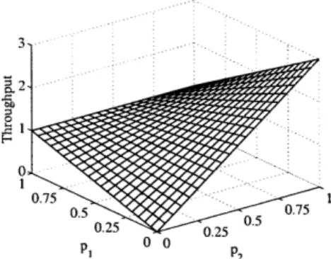
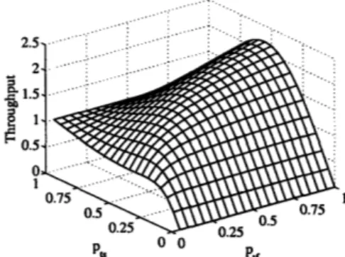
The resulting throughput plot for nl = 1 and n2 = 3 for all values of pl and p2 is

in Fig. 4-2. In this example we use z = 0.2 which corresponds to c = 5, satisfying

nl < c and n2 < c. We see from the figure that the throughput of the system takes its

maximum at the end point (p1, P2) = (0, 1) giving throughput of 1 for each faraway nodes and 0 for the nearby node. This suggest that giving a higher probability of transmission to distant users might yield a higher throughput.

Moreover, we can find the fair point in the plot, i.e., the point which gives the same throughput to all the nodes for n1 = 1 and n2 = 3. The throughput equation is given by

S = pl + (1 - P1)3p2, where nearby throughput is equal to pi and faraway throughput per node is (1- Pl)P2. Equating the two we get, pi = (1- Pl)p2, yielding S = 4_{pl. Notice that}

P2 = Pl/(1 - pi) which means that the fair point requires P2 > pl. Furthermore, P2 • 1 requires pl/(l - pl) < 1 and hence pi < 0.5 yielding S = 4pl < 2 with equality for the point (pl, P2) = (0.5, 1). As a result, the point producing the highest throughput value that is divided evenly between the users is (Pl, P2) = (0.5, 1). Therefore, in this example we see that not only the highest throughput but also the fair point with highest throughput is obtained by giving more chances to faraway nodes.

10C

00 P,

Figure 4-2: Throughput plot for the system in Example-1 for ni = 1, n2 = 3 and z = 0.2.

4.2 Aloha with Two Distances: Example 2

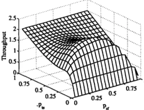
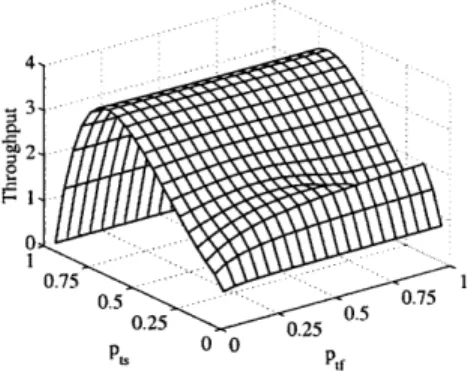
Now consider the same settings as in the previous example but this time with nl = 2 and n2 = 6 in Fig. 4-1. When we choose z = 0.2 and hence c = 5 as in the previous example, nodes at distance 1 are still successful all the time, however nodes at distance 2 can fail if there is a transmission from distance 1 or if all 6 of the distance-2 nodes transmit simultaneously.

Observation 2 Throughput S is maximum at pl = 0 and the maximum value is given by

max

i

(1

p(1

(4.2)

6

i=

)

Then, S = 2_{pl + (1 - pl)}2_{C = C + p1(}2 _{- C(2 - pi)), which takes its maximum value}

of C at Pl = 0 as long as C > 2 Now it is enough to show that for at least one value of

p2, f2(p2) is greater than 2. For P2 = 0.5, f2(P2) = 2.9 > 2. O

0

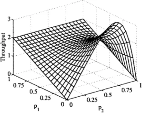
Figure 4-3: Throughput plot for the system in Example-2 for nl = 2 ,n2 = 6 and z = 0.2.

The resulting throughput plot for all values of pi and p2 is in Fig. 4-3. These examples show that giving higher probability of transmission to the faraway users can potentially result in higher throughput values in the multipacket reception channel. The crucial point of the analysis in the examples is assuming n2 > nl, which is reasonable for many spatial

distribution of nodes, for example for a uniform distribution of users on a disk, the number of users increase linearly with the distance from the center of the disk where the receiver is located.

4.3 Backward Protocol with Random Distances and

Sin-gle Capture: Example 3

We utilize the Backward Protocol in this section where there are n nodes randomly dis-tributed on a plane and there is single capture capability at the receiver. We assume the classical vulnerability circle model suggested in [49], [1] and [21], i.e., a transmission from distance r is successful as long as there is no simultaneous transmission within the disk of radius a r. Note that, a is assumed to be greater than 1 in this example and hence there is only single capture in the system. In Section 5.1, we will also demonstrate that the vulnerability circle model can be derived from the power capture model for the case of two nodes as mentioned in [27].

Now we introduce an approximate model which will be revisited in Section 5.2.2 in a more detailed fashion under the name basic approximate model. We assume that at each

transmission attempt, regardless of the number of retransmissions suffered, a packet trans-mitted by a node at distance r is lost with constant and independent probability3 _pd(r). Note that pd(r) is the probability that a node at distance r fails given that it has transmitted. In general, the probability that a packet is lost depends on other transmissions, however, if the number of nodes is large, we expect the approximate results to be close to the exact values. In fact, in Section 5.1, we develop an exact analysis for two nodes and show that the results obtained by the approximate model are very close to those of the exact model even for a small number of nodes.

It can be seen that, regarding the single user state machine in Fig. 3-1, a node changes its state from After Success to After Failure if it attempts and fails in the current slot, i.e., with probability ptPd. Similarly, a node changes its state from After Failure to After Success if it attempts and succeeds in the current slot, i.e., with probability ptf(1 - Pd). The steady state probabilities of the corresponding Markov Chain for a node at distance r can easily be found to be;

PAS

PAS tsPd(T)+ptf(1-Pd(r))

ptspd(r) = PtsPd(r)+Ptf(1-Pd(r))

Next, we can obtain the overall transmission probability, given by

7(r) = PtsPAS + PtfPAF = Ps (4.3)

1 - pd(r) + •pd(r)

The probability that a transmission from a node at distance r fails is the probability that there is at least 1 node transmitting from within the circle of radius or among n - 1 other

nodes in the network. This probability is given by

pa(r) = 1- (1 - T(x) fr (x)dx (4.4)

Where fr(x) is defined by (3.4). Now for any n and any fr(r), (4.3) and (4.4) can be solved

3

This is usually done in the analysis of IEEE 802.11 without the dependence on r (e.g., [17]) and with the dependence on r in [36].

0U. 0.15 0.05 a no 0 0.2 0.4 0.6 0.8 1 Distance, r

Figure 4-4: The transmission probability and the throughput as a function of distance under the forward

(pt, = 0.2 and Ptf = 0.05) and the backward (pts = 0.05 and ptf = 0.2.) backoff mechanisms for a = 2

and uniform distribution of 12 nodes on a disk.

numerically as a system of non-linear equations4. Once T(r) and pd(r) are obtained, S(r) can be easily found by

S(r) = T(r)(1 - pd(r)) (4.5)

Averaging S(r) over all r, we obtain the average throughput of the network;

S = jS(r)fr(r)dr (4.6)

r

Now for N = 12, a = 2 and fr(r) = 2r Vr E (0, 1), Fig. 4-4 presents the values of T(r) and S(r) for the forward model (for pts = 0.2 and Ptf = 0.05) and the backward

model (for pts = 0.05 and pt = 0.2). It can be seen that under the backward model,

the transmission probabilities T(r) of the distant nodes are higher than the transmission probabilities of the nearby nodes. Furthermore, comparing the two models, we see that the transmission probabilities of the distant nodes in the backward model are higher than those of the forward model. This leads to a system that is more fair than the forward model and that provides similar capture probabilities to the nodes regardless of their location. The throughput as a function of distance does not decay much in the backward model, whereas in the forward model, the throughput of faraway nodes is significantly less than that of nearby nodes and since the number of distant nodes is significantly larger than the number of nearby nodes, we expect the overall throughput of both systems to be similar;

4

Note that (4.3) and (4.4) can be solved analytically in the case of two nodes. It is done to verify the numerical analysis and the solution is given in Appendix A for fr(r) = 1 r E [0, 1] and a = 1.

__ Standart model- c(r) .... Standart model-S(r) S - Alternative model--t(r) - - - Alternative model-S(r) .. .- •2 . . -_ . . . . -- -,,i. . . .:. . . S i * __ _ t__ __ _

for instance, for the example of Fig. 4-4, the throughput of the forward model is 0.4617 and that of the backward model is 0.4343.

In the light of these examples, even in a single capture channel, the backward model achieves more fair results for distant users and can potentially provide better throughput characteristics than the forward model. We naturally expect this to hold even more strongly with multipacket reception capability.

Chapter

5

Protocol Analysis

In this section we analyze the backward protocol for various different settings. We first de-velop an exact analysis of the Backward Protocol when nodes are randomly distributed on a disk and there is no multipath fading in the channel. The analysis enables us to verify the approximation we used in Section 3.1. Then we move on to a case where the node locations are known in advance. We introduce a more powerful approximation that can be utilized only in deterministic node locations case and use it to extend our analysis to networks with more users and more possible distances from the receiver than the exact analysis. Next we consider the above cases when there is multipath fading in the system. We utilize previous approximate models to both the deterministic node locations with fading and random node locations with fading cases and get analytical results. We show by numerical analysis that the backward model yields more fair results in all the cases and greater throughput in most of the cases compared to the forward model.

5.1 Random Locations Without Fading

In this section we develop an exact analysis using Markov Chains for the case where the node locations are random and there is no fading in the system. Our objective is to show that the approximate results used in the third motivating example in Sec. 3.1 are very close to the exact results even for a small number of nodes in the network. The approximation we used was that regardless of the success history, a packet from a user at distance r is