Dynamics of Automobile Ownership Under Rapid Growth

Dynamics of Automobile Ownership Under Rapid Growth

The MIT Faculty has made this article openly available.

Please share

how this access benefits you. Your story matters.

Citation

Zegras, P., and Veronica Hannan. “Dynamics of Automobile

Ownership Under Rapid Growth.” Transportation Research Record:

Journal of the Transportation Research Board 2323 (December

2012): 80–89.

As Published

http://dx.doi.org/10.3141/2323-10

Publisher

Transportation Research Board of the National Academies

Version

Original manuscript

Citable link

http://hdl.handle.net/1721.1/100765

Terms of Use

Creative Commons Attribution-Noncommercial-Share Alike

The Dynamics of Automobile Ownership Under Rapid Growth:

The Santiago de Chile Case

P. Christopher Zegras

Massachusetts Institute of Technology Department of Urban Studies and Planning 77 Massachusetts Avenue, Room 10-403 Cambridge MA 02139

Email: czegras@mit.edu Phone: 617 452 2433 Fax: 617 258 8081 Veronica Adelle Hannan

Massachusetts Institute of Technology Department of Civil Engineering /

Department of Urban Studies and Planning 77 Massachusetts Avenue, Room 1-235 Cambridge MA 02139

Email: vhannan@mit.edu Phone: 504-912-6591

Revised Version 15 March 2012

For publication in Transportation Research Record

ABSTRACT

Little research has focused on how factors influencing travel behavior change in rapidly developing and motorizing cities. We examine the case of household motor vehicle ownership, focusing on potential variations in preferences revealed through vehicle choice models estimated for Santiago de Chile in 1991 and 2001, and including measures of relative location, metro proximity, residential density, and land use mix. The results indicate that preferences have changed from 1991 to 2001, suggesting that as incomes rise and vehicle ownership becomes increasingly affordable, demographic and land-use and other contextual variables change in their apparent influence. The results vary across land use and locational variables; most notably the relationship between vehicle ownership and land use mix appears to weaken over time, while the distance to CBD effect strengthens, and the residential density effect varies in the apparent direction of change, depending on the vehicle ownership category. An effect of proximity to Metro apparently emerges by 2001 for the household decision to own 3 or more vehicles. This research shows that although income and motorization rates rapidly increased in Santiago, certain elements of the built environment influence household vehicle ownership, and these influences change over time. Future research should focus on potential market segments, such as suburban versus urban, aim to control for self-selection regarding the land use and locational characteristics, and better understand the implications for travel forecasting.

INTRODUCTION

The growth in motor vehicle fleets arguably poses as the single most important factor influencing

developing countries’ mobility and accessibility. Most persons want the convenience, status, and comfort of private motorized travel, but in aggregate these desires translate into well-documented problems. The potent force of global motorization raises numerous interesting questions. Does a foreseeable ceiling exist for motorization (vehicles per capita) in cities of the developing world? Will resource constraints or the accumulation of externalities attenuate motorization? Do the dynamics of vehicle ownership structurally change cities? Do the dynamics of urban growth change vehicle ownership preferences and trends? We set out to shed some light on the last of these questions, examining the case of Santiago de Chile, during the 1990s. International comparative evidence shows a strong relationship between income and motorization (1). In much of the developing world, the vast majority of the population is still at income levels well below the minimal vehicle ownership threshold. This situation is changing, however, as incomes rise and vehicle prices fall, spurred in part by entrance into the international motor vehicle production market of companies from countries like China and India as well as international trade of used vehicles (2).

Within a country or city, the same income-ownership relationship exists, but at this finer resolution the influences of local policies and other more nuanced factors appear. In Chile, for example, household vehicle ownership data suggest that cities within “free trade zones” (import-tariff-free) – Punta Arenas, Iquique, Arica – have the lowest share of zero-car households in the country (3). Other local policies, not originally aimed at affecting vehicle ownership per se, also play a role. For example, Mexico City’s “Hoy No Circula” program, a restriction on driving by certain vehicles (based on license plate numbers) during high pollution days, created the perverse impact of promoting the purchase of an additional second hand vehicle (apparently imported from other parts of the country) by many families (4). The government more recently adapted the ban to create an incentive for purchasing cleaner vehicles, an approach also adapted in the case of Santiago, which uses a similar restriction policy.

Evidence also suggests a relationship between household automobile ownership and relative transportation levels of service and urban form and design. In fact, increasing motorization and its attendant impacts may further induce motorization (5). For example, motorization fuels spatial

decentralization, which in turn drives motorization. Further, while motorization exacerbates congestion, congestion may then create the perverse incentive of increasing automobile ownership and use.

Increasing congestion further encumbers main arteries, slowing buses and other surface transit relative to private cars which can choose less congested alternative routes and/or destinations (5). Zegras (6) finds, for the Santiago case in 2001, that household vehicle ownership can be partly explained by the

household’s relative location in the city, distance to metro stations, relative accessibility levels between auto and bus, and various neighborhood design characteristics, including density and land use mix.

Concerns about motorization relate not only to the overall magnitude – that is, the total motor vehicle fleet size – but also the rate of increase, which may outpace relevant physical and institutional capabilities. Ultimately, motorization is a driving force behind increases in transportation greenhouse gas and local pollutant emissions, pressures for land conversion to urban uses, dependency on petroleum, and demands for infrastructure expansion. In the face of these challenges, in this paper we take on a relatively modest topic, attempting to discern apparent changes in household vehicle ownership preferences. Specifically, we look at households in Santiago, in 1991 and 2001, estimating and comparing vehicle ownership models. The following section describes the modelling approach. The third section briefly introduces the empirical setting. The fourth section presents the model estimations and discusses the results. The final section concludes.

VEHICLE OWNERSHIP MODELING

Two basic approaches to household vehicle ownership exist, aggregate and disaggregate, as reviewed in detail by de Jong et al (7). Aggregate analyses model vehicle ownership at zonal, urban, or national levels, and can be used for inputs into travel forecasting models, and/or for intra-city, inter-city, or international comparative efforts, to derive, say, the income elasticity of demand for motor vehicles, and/or develop forecasts of future vehicle fleets. Such models generally use ordinary least squares (OLS)-type regression models.

Disaggregate models, on the other hand, typically use household-level data to examine more detailed behavioral relationships at the decision-maker level. Disaggregate models comprise a range of types, depending on purpose and data availability (7). The most basic, static vehicle holding models aim to predict the number of cars owned by a household at a given time (i.e., cross-sectional) and can reveal effects of relevant household characteristics, such as number of employed adults, and household

locational attributes, such as distance to central business district and local land use mix (6). More refined static models focus on vehicle type (e.g., “alternative fuel”) and can contain a number of vehicle-specific attributes like operating costs and top speed (8). These disaggregate approaches, catching a single glimpse in time, can be used to develop long run forecasts with fairly moderate data demands (7); however, they do not capture more fine-grained behavioral dynamics, such as the timing of decisions about new vehicle purchases, vehicle disposal, additional acquisitions, and so on (9). Dynamic disaggregate models aim to model such effects explicitly over time, utilizing household panel (or pseudo-panel) data (10). Such approaches can reveal changes due to lifestyles, cohort effects, vehicle prices, fuel prices, etc. and enable both short- and long-term forecasting; the challenges lie in their data requirements (7).

Published research on disaggregate vehicle ownership modeling in the developing world remains somewhat limited. Wu et al. (11) model auto ownership in Xi’an, China based on a 1997 survey,

developing and operationalizing the concept of “symbolic utility,” or psychological satisfaction, in the ownership model. The results support the role of “symbolic utility” in influencing vehicle ownership, although income dominates; they also indicate a significant role of bus stop accessibility and

neighborhood parking availability. Dissanayake and Morikawa (12) model automobile and motorcycle ownership in a nested logit model of vehicle ownership, mode choice, and trip chaining in Bangkok using 1995-96 data. Srinivasan et al. (13) model the change in vehicle ownership, as reported retrospectively by respondents to a 2004-2005 household survey in Chennai, India. Using an ordered probit model, they find car ownership is positively associated with parking proximity, home ownership, peer pressure, and social connectivity and negatively associated with grocery store proximity. Li et al (14) model household vehicle choice in Chengdu and Beijing, China, using logit on data for 2005 and 2006, respectively. They find population density to be negatively associated with auto ownership in both cities and, in contrast to studies in the West, that the likelihood of vehicle ownership declines with greater distance from the CBD. As discussed in the introduction, Zegras (6), using a multinomial logit model with data for Santiago in 2001 finds a number of transport level-of-service, relative location, and built environment variables to be related to vehicle ownership. We use that same dataset for the 2001 model applied below.

Modeling Approach

Analyzing household vehicle ownership in four different datasets, Bhat and Pulugurta (15) find that the unordered (i.e. MNL) model outperforms an ordered response model (according to several measures of fit), leading them to conclude that the unordered response choice mechanism is a better representation of the household auto ownership decision (consistent with global utility maximization). In the traditional MNL model, a decision-maker, faced with multiple alternatives, chooses that which provides the greatest utility, with utility itself viewed as a random variable. Assuming a logistically distributed error term (εn), we can estimate the probability of choosing alternative i as (16):

𝑃𝑛(𝑖) = Pr⁡(𝑈𝑖𝑛 ≥ ⁡ 𝑈𝑗𝑛) (1),

= ⁡ 𝑒

𝜇𝑉𝑖𝑛

𝑒𝜇𝑉𝑖𝑛 +⁡𝑒𝜇𝑉𝑗𝑛

where:

𝑃_𝑛(𝑖) is the probability of decision-maker n choosing option i; 𝑈_𝑖𝑛 represents the random utility of option i to decision-maker n; 𝑈𝑗𝑛 represents the random utility of option j to decision-maker n;

𝑉_𝑖𝑛 represents the systematic utility of option i to decision-maker n; 𝑉𝑗𝑛 represents the systematic utility of option j to decision-maker n; and,

𝜇 is a positive scale parameter arbitrarily assumed to be one.

In this formulation, 𝑈_𝑖𝑛 = 𝑉_𝑖𝑛+ 𝜀_𝑖𝑛 and 𝑈_𝑗𝑛= 𝑉_𝑗𝑛+ 𝜀_𝑗𝑛, with 𝜀_𝑖𝑛 and 𝜀_𝑗𝑛 representing the random disturbances.

Our interest is in examining the stability of vehicle ownership decision-making over time: we want to compare models from two different time periods, 1991 and 2001. Doing so requires ensuring that any observed differences from model estimation do not actually derive from variances in the underlying data; we must account for potential differences in the magnitudes of the random error component

variability. Such an approach allows distinguishing between differences in model parameter estimates that arise from different error variances and those that arise from real differences in the model parameters (17). Specifically, as discussed for Equation (1), the scale parameter, µ, cannot be identified and is arbitrarily assumed to be one, an assumption with no effect on the utility order within a particular dataset. Between datasets, however, the values of the scale parameters may differ significantly, implying

variability across the datasets. Although µ cannot be identified in a single data source, the ratio of the µ’s from different datasets can be estimated, relative to an arbitrary reference.

As such, when comparing parameters from models in different times, one must account for the possible differences in error component variances. Following Severin et al. (17), consider β91 and β01 to represent, respectively, vectors of parameters for choices in datasets from 1991 and 2001, and µ91 and µ01 to represent the respective scale parameters. If the differences in parameter estimates arise from variance scale ratios not equal to one, as opposed to actual differences in the β’s, then β91 = β01 and µ91/µ01 ≠1. In other words, if estimation produces different model parameters over two periods, one might infer that the effects of common observed factors (e.g., income) have changed over time, when the difference actually comes from the variance scale ratio (µ01/µ91). These differences can be tested via different model estimations, specifically: (1) estimating separate models for each dataset (allowing different parameters for each) and, then, (2) estimating a single model with the combined dataset, restricting the parameter values (β’s) to be identical but allowing for different variance scale ratio parameters (µ’s) for each dataset. The preferred model – either (1), the “unrestricted” model or (2) the “restricted” model – can be determined by applying a likelihood ratio test. This approach is known as the stability of preferences test.

EMPIRICAL CASE: SANTIAGO DE CHILE

Santiago is the capital of one of Latin America’s most consistently growing economies. The country has sustained strong economic growth since its return to democracy in 1990, and entered into the OECD as of 2010. Santiago concentrates a large share (greater than 40%) of the nation’s population, jobs, and wealth.

Since our analysis focuses on the vehicle ownership changes between 1991 and 2001 the following description primarily concerns basic city dynamics in that period.

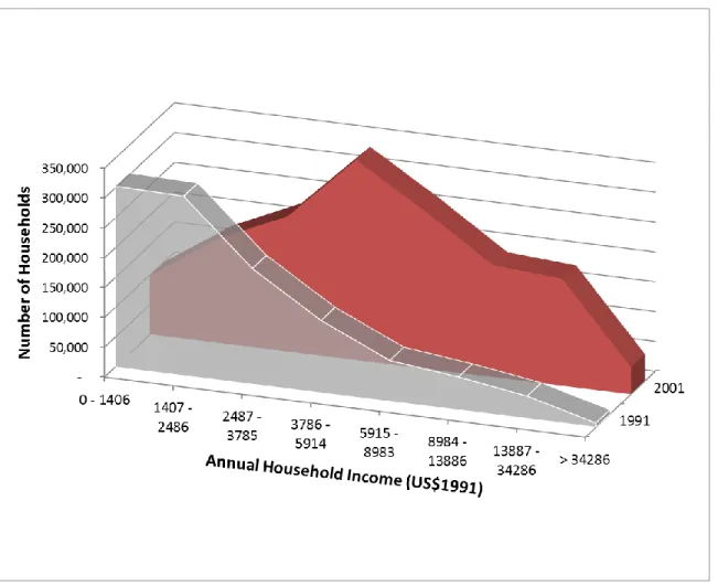
From 1991 to 2001, the greater metropolitan area experienced a mean annual growth in average household income of 6.5%, from US$ 4,700 to US$ 9,000 (in US$2001). By 2001, a burgeoning middle class was evident (see Figure 1). Nonetheless, while by 2001 over 50% of the households earned, on average, between US$6,000 and $13,000 per year, a large share still earned less than $4,000 per year. In fact, 15% of the households earned, on average, less than the minimum monthly wage (equivalent to approximately $2,400 per year), just enough income for subsistence (the average household size in this income stratum is 2.95; the per capita subsistence cost is $36 per month). On the other extreme lies the wealthy – a small share of Santiago’s households in 2001 already enjoyed average incomes on par with the industrialized world, with 5% of the households earning on average roughly the same income as the median US household in 2003. Santiago’s residential geography has historically been characterized by socioeconomic spatial segregation, a pattern moderating somewhat in recent years (18).

Land Use and Transportation Characteristics: 1991 to 2001

In terms of physical structure, Santiago began experiencing accelerated urban expansion in the early 1980s, when the city-wide population density began declining more rapidly than in any other period of the previous 50 years, influenced by factors like road-building, low density suburban subdivisions, distant public housing projects, and industrial relocations (19). By the mid-1990s a new CBD emerged, 4.5 kilometers east of the traditional CBD, giving the city an emerging duo-centric business core, linked by a major commercial thoroughfare. Office parks and shopping malls were already apparent on the urban fringe by 2001.

Residential dwelling characteristics largely match spatial income distribution patterns, with low income areas associated with high dwelling unit densities. The primary exception comes from the high densities of large apartment buildings in the traditional and eastern CBDs and apartments continuing to sprout up in the wealthier east. Land use mixes largely radially follow he primary commercial arterials, with large swaths of areas with low land use mix across the city. The historical grid pattern street still predominates, until one gets fairly distant from the center of the city, most notably in the far Eastern foothill suburbs. Zegras (18) provides more detailed analysis of Santiago’s urban structure, form and design. Urban growth in Greater Santiago is regulated by an inter-municipality land use plan; an update to the 1960 plan was approved in 1994; the 1994 was subsequently modified in 1997 to add 19,000

urbanizable hectares (approximately 35% of the metro area’s urban area at the time) in the north of the metro area (19).

As would be expected, Santiago’s changing socio-economic characteristics and physical form have impacted household travel behavior. The motorization rate (vehicles per 1000 persons) increased by over 4% per year over the period 1991-2001 (although in 2001 it still stood at only 20% of the US level and just 30% of Western European levels), while private motorized mode share increased even more rapidly (almost 7% per year) and public transport mode share declined (by 3% per year) (6). In 2001, Santiago still enjoyed remarkably ubiquitous bus service, while the Metro coverage was obviously more limited; not an insignificant fact, since for most periods of the day walking provides the primary means of Metro access and egress (20).

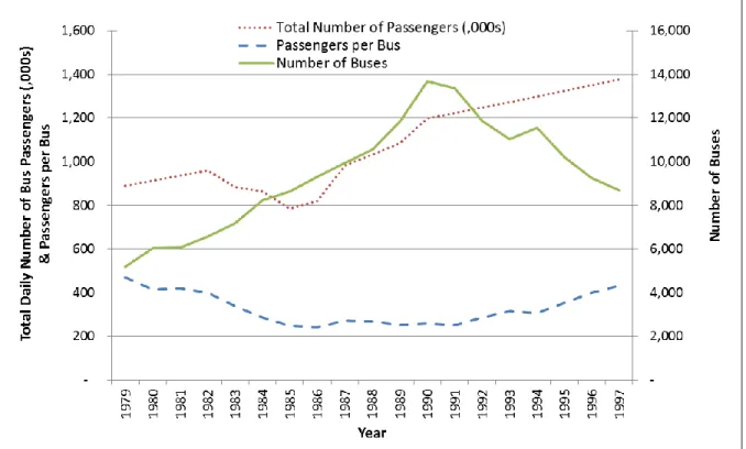
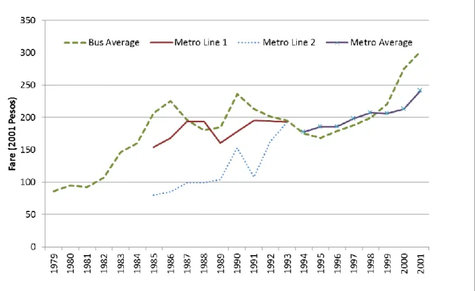
In the past 40 years, the Santiago bus system changed dramatically. In the 1970s and 1980s service provision and fares were completely deregulated. The early 1990s brought the gradual re-introduction of regulation for road-based public transportation, producing incremental improvements in the quality of the bus system via the route concessions tendered in 1992, 1994, and 1998. The results included: reduced overall number of vehicles (from a high of approximately 14,000 in 1992 to 9,000 in 2000) (Figure 2), stabilized fares (see Figure 3), and improved service quality (21). Nonetheless, the system remained loosely regulated, marked by atomized ownership structure, competition in the streets for passengers, fairly unsafe operations, congestion and air pollution, and an important degree of

collusion among the companies (18). Moreover, fares on the system were not integrated, neither between buses nor between buses and the Metro, making transfers expensive. By 1999, the bus system carried 4.7 million passengers per day (22) and operated without any direct government subsidy. Most recently, and perhaps most famously (and/or notoriously), in 2007 Santiago launched a massive and single-stroke

reform of its public transportation system, known as Transantiago. As this reform occurred after the time period of interest to us, we do not detail it here. Interested readers should consult Muñoz and Gschwender (23).

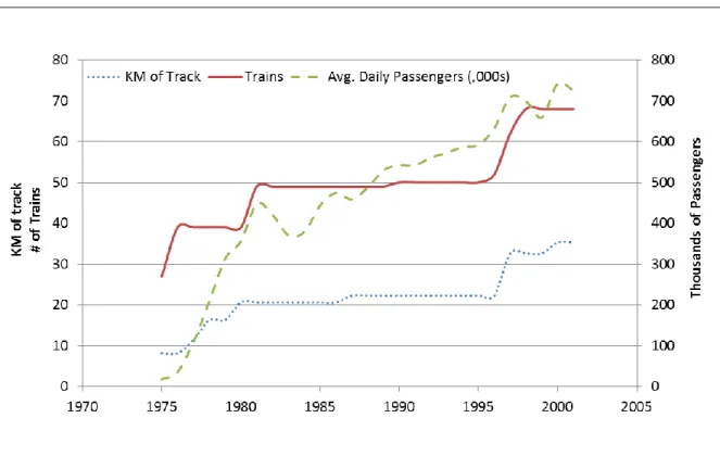
Santiago’s original two Metro (urban heavy rail) lines were completed at the end of the 1970s, totaling approximately 27 kilometers and 37 stations. A third Line (known as Line 5) was brought into service in 1998 (see Figure 4) adding 13 kilometers and 15 stations. By 2001 the system carried an average 725,000 passengers per work day (20). In 1991 Metro lines 1 and 2 had two separate fares, and a transfer from line 2 to line 1 required an additional fee (Figure 3). In 1994, an integrated, differential fare for both lines replaced the separate fee system, which likely improved customer experience.

Despite a history of relative demand management-focused transportation planning, by the early 1990s, large-scale roadway upgrades began and by the late 1990s plans were in place for Chile’s highway concessions program to bring large investments to highway upgrades and expansions in the city.

Nonetheless, by 2001 none of the concessioned highways had yet entered operations. By one estimate, Santiago in 2001 had a slightly smaller share of its urban area dedicated to highways as Chicago in 1956 (2.1% versus 2.8%), when that city was just at the beginning of the massive highway investments that would come via the USA Federal highway investment program (18).

HOUSEHOLD MOTOR VEHICLE CHOICE IN SANTIAGO: 1991 VERSUS 2001

Data Sources

Data for this analysis come from the 1991 and 2001 household origin and destination (OD) surveys carried out for the national transportation authorities (SECTRA). The surveys benefit from consistency in implementation approach, team, and authority (24, 25) and benefit from the long tradition of

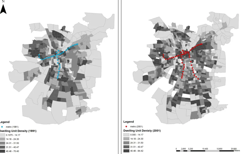
transportation engineering excellence in Chile. The 1991 survey was based on a randomly generated sample of approximately 32,000 homes surveyed in April, May and June (in total, 3% of Greater Santiago’s households). The urban area included 34 comunas (municipalities) distributed over 420 km2 (see Figure 5). The region was divided into 409 OD survey zones, ranging in size from 18 to 27,000 hectares, with an average of 478 hectares. The 2001 survey was based on a smaller sample of 15,000 households, of which 12,000 were surveyed during the normal work/school season and 3,000 during summer time (in total, 1% of household in the Santiago Metropolitan area). The urban area had also expanded to include 38 comunas distributed over 2,000 km2, and further divided into 778 OD zones, ranging in size from 17 to 19,000 hectares with an average of 250 hectares.

Both surveys contained information on family size, reported income, and number of vehicles per household, as well as each family member’s job status. In 1991, income was reported by income

categories; the 2001 survey recorded reported monthly income. To minimize the differences between each data set, all 2001 incomes were deflated to 1991 values, using the official consumer price index for Chile, and assigned a corresponding income bracket from the 1991 survey. The household survey information was geo-coded to the OD zone level for the 1991 data, and to the center of each census block for the 2001 data. For this analysis, only OD zone level characteristics were considered, for consistency. Lastly, both surveys included expansion factors that related the characteristics of the sample population to Greater Santiago’s actual population characteristics. These expansion factors were used to determine the number of dwelling units per OD zone in the dwelling unit density calculation.

Land Use Variables and Accessibility Proxies

A consolidated form of the 1991 and 2001 national tax records data is available on SECTRA’s website (26). It aggregates all land-use to the travel model (ESTRAUS) zones and into 5 general categories (e.g., residential, commercial, educational), providing the m2 of constructed area for each registered activity. This information was used to characterize land uses within the OD zones by joining the ESTRAUS zones to each year’s corresponding OD zones.

Local land use mix was measured through a diversity index, following Rajamani et al. (27). The diversity index, DI, is calculated as:

𝐷𝐼 = 1 − [

]

r = square meters of residential floor space; c = square meters of commercial floor space; e = square meters of education floor space; s = square meters of services floor space; i = square meters of industrial floor space; and, T = r + c + e + s + i.

This measure attempts to capture the relative mix of uses in a given zone: a value of 0 implies that the zone is single use, while a value of 1 indicates that the land is perfectly divided among all five uses. Theoretically, the mix of uses generates different transportation demands for the zone’s residents; we would expect, all else equal, that higher land use mix would be associated with lower household vehicle ownership.

Lacking comparable transportation levels of service measures for the two years studied, we test relatively crude measures of accessibility: the household OD zone centroid’s distance to the traditional CBD (in meters); and if the household OD zone centroid is within 500 meters of a metro station.

As discussed, the city expanded outward considerably over the 1991-2001 period, and the 2001 household survey covers this broader expansion area, especially to the rapidly suburbanizing North. Nonetheless, we restrict our analysis to a common geography for the two years, to control for motor vehicle ownership effects that might be unique to the newly formed distant suburbs in 2001; we discuss the implications of this restriction below.

Data Summary

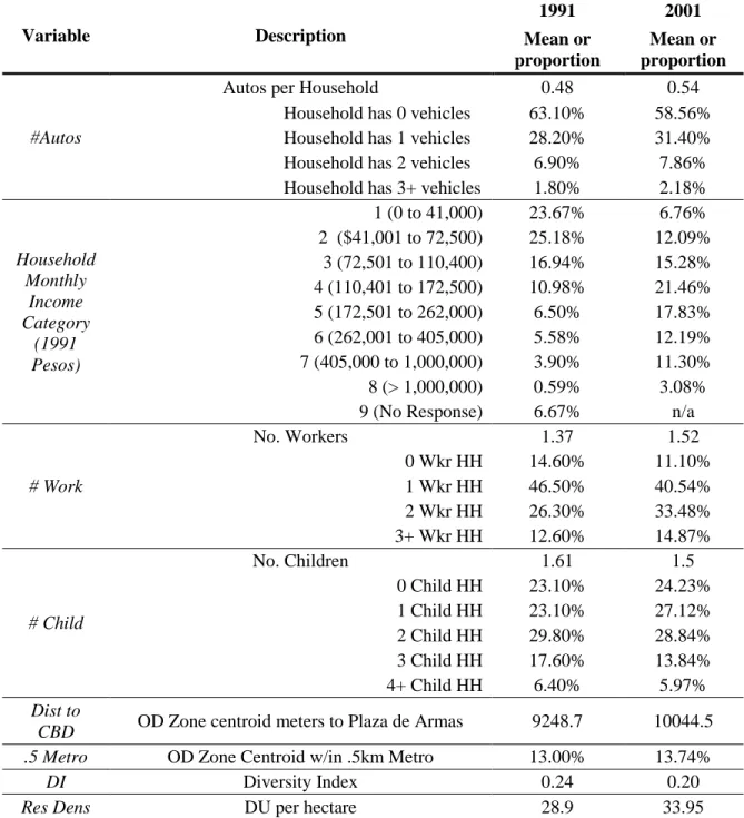
Table 1 presents the variables used in the models and their descriptive statistics. The data reveal the increase in household incomes and the larger concentration of households in the middle income groups (seen also in Figure 1). Consistent with this, the share of zero-car households decreased by 5%; the largest increase was in one-car households. Labor participation increased modestly as 0 worker and 1-worker households declined (consistent with increased women in the workforce), while 2 and 3 1-worker households increased. The number of children per household decreased slightly, with more households having one child in 2001 and fewer having three children.

In terms of land use characteristics and relative location, the average zonal distance to the CBD increased by about 800 meters – households are moving outward even within the same geographical area. Despite the expansion of the metro network, the share of zones within 500 meters of a metro station increased by less than one percent. Finally, average zonal density increased by 5 dwelling units per hectare, likely reflecting the growth in apartment building construction, particularly in the inner-Eastern parts of the city (see Figure 5); while average zonal land use mix slightly declined.

Model Results

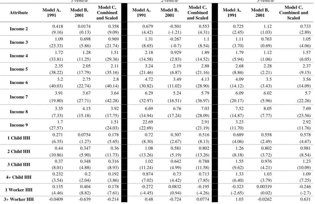
We model the household decision to own 0, 1, 2, or 3+ vehicles via a multinomial logit (MNL) model and applying the stability of preferences test as described above. We first estimate two unrestricted models that allow for different parameters for each data set (first two columns in Table 2, Model A and Model B). We then combine the two datasets and restrict the coefficients to be identical, but allowing for different scale parameters for each data set (Model C, Table 2). The log-likelihood ratio test suggests, that although the variance differs, modestly, across the two data sets (significance of the scale parameter in Model C), the unrestricted (separate) models represent a better model fit than the restricted. This result suggests that preferences for household vehicle ownership have changed over the 10-year period.

Comparing the differences between the model coefficients from 1991 and 2001 offers some indication of which variables have changed the most vis-à-vis their relationship with the household vehicle ownership

decision. Technically, to be fully comparable, the 1991 parameter estimates should be divided by the scale parameter estimate (1.13).

In most cases, the parameters carry the predicted signs and are statistically significant. Moreover, similar patterns exist between the parameters estimated in 1991 and those for 2001, indicating relative consistency in the data and analytical approach. Beginning with basic socio-economic characteristics, we see that higher income brackets have a positive and significant effect, as hypothesized. Higher income brackets also progressively increase the likelihood of owning multiple cars, which again, follows intuition. Generally, income had a stronger effect in 1991 than 2001, most notably in the lower income brackets; interestingly, although income was always positive and significant for 1991, in 2001 the lower-income brackets have less significance. This may, in part, be due to unobservable differences in the lowest income categories associated with 2001, which are a much lower share of the population than in 1991 (due to having to use the 1991 income categories for consistency across the two years). Household demographics also play largely expected roles, albeit apparently changing, in vehicle ownership. In both 1991 and 2001, for each number of children, the likelihood of owning more cars increases (i.e.,

parameters tend to increase across vehicle ownership categories for a given number of kids); for each vehicle ownership category, the number of children increases the ownership likelihood, although this effect plateaus. The general tendency is that the strength of the children effect declined from 1991 to 2001. The relationship between number of workers per household and vehicle ownership is more difficult to generalize. One worker had a positive association with owning one vehicle, but a negative one with owning two or three vehicles in 1991. In 2001, one worker had a positive relationship with owning one vehicle, but an insignificant one vis-à-vis owning 2 or more vehicles. In both 1991 and 2001, the 3-plus worker variable had a negative effect on owning 1 vehicle, but varying relationships with owning 2, or 3+ vehicles. For 2 vehicles, 3-plus workers had a positive and significant effect in 1991, but a negative, though equally significant effect in 2001. For the 3+ vehicle choice, the positive relationship in 1991 becomes insignificant by 2001. More nuanced understanding of these relationships is necessary, possibly bolstered by qualitative analysis of vehicle choice processes within different household types.

With respect to the land use variables, land use mix had a negative relationship with all vehicle ownership categories in 1991 but this largely became insignificant by 2001, a result worth further examination. Dwelling Unit Density had a negative and significant effect on vehicle ownership in 1991 and 2001 as was hypothesized. The density effect increased in magnitude for the first vehicle choice, decreased for the second, and remained virtually unchanged for the third. Again, further examination is warranted.

Regarding the accessibility proxies that were used in this analysis, distance to CBD consistently associates with a higher likelihood of vehicle ownership, a relationship that strengthens with the number of vehicles chosen and that strengthens over time. In other words, households further away from the city center have higher likelihood of owning more cars and this effect has increased over time. Controlling crudely for residential density and land use mix and household demographic characteristics, the suburbs apparently became more automobile-conducive. The quadratic of distance to CBD is also significant, however, suggesting a sub-centering effect – households very far from the CBD have a lower likelihood of vehicle ownership. Again, this relationship strengthened over time, perhaps indicating a perceived consolidation of sub-centers and/or other unobserved aspects of the periphery reducing vehicle ownership propensity. We tested various measures attempting to segment the distance to CBD effect by income category, but the more straightforward model implemented here proved the best model fit. Finally, the Metro effect, or lack thereof, is somewhat surprising. In 1991, no significant relationship between Metro proximity and household vehicle ownership emerges. In 2001, a marginally significant negative effect is detected for the 2 vehicle choice and a modestly significant and negative effect (on the order of having one child) is detected for the 3+ vehicle choice.

Limitations and Further Research

Our analysis faces a number of limitations. Most notably, the land use relationships identified may be a product of residential self-selection – meaning that households may choose their locations based on vehicle ownership preferences, at least in part. This may be confounding, for example, the strong

example, joint residential and vehicle ownership models. In addition, the estimation process showed that the results were somewhat sensitive to the changing geographies over the two time periods, especially the emergence of distant suburbs in 2001 which were excluded from this analysis. Further research might also: examine various market segmentation approaches, by income, demographic and other household characteristics, and/or relative location; or more effectively control for transportation levels of service variations, although doing so would require historical network performance data. Furthermore, what we detect and call variation in preferences between the two model years may, in fact, be due to non-linear effects that are not captured by the null hypothesis of changes in the model coefficients. Finally, more work is clearly needed to understand the policy and planning implications of these model results, including accounting for temporal changes in behavioral parameter estimates in simulations.

CONCLUSIONS

We examined whether household vehicle ownership preferences have changed over a 10-year period in a rapidly developing city that has undergone important transportation system, urban development, and income changes. Our results demonstrate that preferences influencing vehicle choice models have, in fact, changed. The results suggest some interesting variations in relative influences among socio-economic and demographic factors and land use and locational variables. Among lower income groups, the models show a decreasing tendency for vehicle ownership, possibly due to improvements in public transportation during the 1990s in Santiago. The improved overall quality of service may have been notable enough to allow the lowest income brackets to prefer to depend on transit for their mobility needs.

Among the land use variables, we see countervailing changes – on the one hand, the influence of land use mix, while still negatively correlated with vehicle ownership, declines over time. The opposite trend appears in the case of distance to CBD. The effective of residential density changes modestly, while a slight proximity to Metro effect appears to emerge for the three vehicle choice by 2001.

The results suggest that household preferences for vehicle ownership are dynamic over time and that they respond to the rapidly developing and evolving environments around them. Nonetheless, the research raises a number of questions and areas for further investigation, including the role of self-selection, market segmentation, and policy and planning implications.

ACKNOWLEDGMENTS

We thank SECTRA for providing the data and several reviewers for very useful comments.

REFERENCES

1. Ingram, G.K. and Liu, Z. ‘Vehicles, Roads, and Road Use: Alternative Empirical Specifications’ (Policy Research Working Paper 2036), Washington, DC, World Bank, 1998.

2. Zegras, C. Used Vehicle Imports in Perú: Effects on Motorization, Energy and Emissions, International Institute for Energy Conservation, Washington, DC, 1998.

3. SECTRA, Indicadores de movilidad, 2011, data downloaded from:

http://www.sectra.cl/Indicadores_de_Movilidad/indicadores_movilidad.html.

4. Eskeland, G. and Feyzioglu, T. ‘Rationing Can Backfire: The ‘Day without a Car’ in Mexico City’, The World Bank Economic Review, 11, 1997, 383-408.

5. Gakenheimer, R., ‘Urban mobility in the developing world’, Transportation Research Part A, 33, 1999, 671-689.

6. Zegras, C. The Built Environment and Motor Vehicle Ownership and Use: Evidence from Santiago de Chile. Urban Studies, 47 (8), 2010, 1793-1817.

7. de Jong G, Fox J, Daly A, Pieters M, Smit R, “Comparison of Car Ownership Models” Transport Reviews 4(4), 2004, 379-408.

8. Brownstone D, Bunch D, Train K, “Joint mixed logit models of stated and revealed preferences for alternative-fuel vehicles” Transportation Research Part B 34(5), 2000, 315–338.

9. de Jong G, Kitamura R, “A review of household dynamic vehicle ownership models: holdings models versus transactions models” Transportation 36, 2009, 733–743

10. Hanly, M, Dargay, J, “Car Ownership in Great Britain: Panel Data Analysis” Transportation Research Record 1718, 2000, 83-89.

11. Wu, G, Yamamoto, T, Kitamura, R, “Vehicle Ownership Model that Incorporates the Causal Structure Underlying Attitudes Toward Vehicle Ownership” Transportation Research Record 1676, 1999, 61-67,

12. Dissanayake, D, Morikawa, T, “Household Travel Behavior in Developing Countries Nested Logit Model of Vehicle Ownership, Mode Choice, and Trip Chaining” Transportation Research Record 1805, 2002, 45-52.

13. Srinivasan, K, Bhargavi, PVL, Ramadurai, G, Muthuram, V, Srinivasan, S “Determinants of Changes in Mobility and Travel Patterns in Developing Countries: A Case Study of Chennai” Transportation Research Record, 2038, 2007.

14. Li, J, Walker, J, Srinivasan, S, Anderson, W, “Modeling Private Car Ownership in China:

Investigation of Urban Form Impact Across Megacities” Transportation Research Record 2193, 2010, 76-84.

15. Bhat C, Pulugurta V, “A comparison of two alternative behavioral choice mechanisms for household auto ownership decisions” Transportation Research B 32(1), 1998, 61-75.

16. Ben-Akiva M, Lerman S, Discrete Choice Analysis-Theory and Application to Travel Demand (MIT Press: Cambridge), 1985.

17. Severin V, Louviere J, Finn A, “The stability of retail shopping choices over time and across countries” Journal of Retailing 77, 2001, 185-202

18. Zegras, C. Sustainable Urban Mobility: Exploring the Role of the Built Environment. PhD

Dissertation submitted to the Department of Urban Studies and Planning, Massachusetts Institute of Technology, Cambridge, MA, September, 2005.

19. Zegras, C. and R. Gakenheimer. Urban Growth Management for Mobility: The Case of the Santiago, Chile Metropolitan Region. Working Paper for the Lincoln Institute of Land Policy and the MIT Cooperative Mobility Program, Cambridge, 2000.

20. Metro, S.A. Statistical Appendix 2001. Metro de Santiago, Santiago, 2001.

21. Dourthé, A., H. Malbrán, M. Wityk. Santiago de Chile’s Experience with the Regulation of the Public Transport Market. Paper prepared for the 79th Annual Meeting of the Transportation Research Board (TRB), Washington, DC, January, 2000.

22. SECTRA. Datos y Estructura del Sistema de Transporte de Santiago. Santiago, 2000.

23. Muñoz, J.C., Gschwender, A. Transantiago: A Tale of Two Cities. Research in Transportation Economics 22, 2008, 45–53.

24. Ortúzar, JdD, Ivelic, AM, Malbrán, H, Thomas, A “The 1991 Great Santiago origin-destination survey: methodological design and main results” Traffic Engineering and Control, Vol. 34, No. 7/8, 1993, 362-368.

25. Ampt, ES ,Ortúzar, JdeD “On Best Practices in Continuous Large-scale Mobility Surveys” Transport Reviews, Vol. 24, No. 3, May, 2005, 337-363.

26. www.sectra.cl.

27. Rajamani, J. C. Bhat, S. Handy, G. Knaap, Y. Song. Assessing Impact of Urban Form Measures on Nonwork Trip Mode Choice After Controlling for Demographic and Level-of-Service Effects. Transportation Research Record 1831, 2003, pp. 158-165.

List of Tables and Figures

TABLE 1 Variables, Definitions, and Descriptive Statistics

TABLE 2 Motor Vehicle Ownership Model Results FIGURE 1 The Emergence of a “Middle Class City”?

FIGURE 2 Bus Ridership and Fleet Growth During 1980s and 1990s.

FIGURE 3 Evolution of Bus and Metro Fares in Greater Santiago: 1980s and 1990s (20).

FIGURE 4 Metro Ridership and Infrastructure Growth in Time: 1970s to 1990s (20).

FIGURE 5 Modeled Areas in 1991 (left) and 2001 (right): OD Zones, Densities, and Metro Stations.

TABLE 1 Variables, Definitions, and Descriptive Statistics Variable Description 1991 2001 Mean or proportion Mean or proportion #Autos

Autos per Household 0.48 0.54

Household has 0 vehicles 63.10% 58.56% Household has 1 vehicles 28.20% 31.40% Household has 2 vehicles 6.90% 7.86% Household has 3+ vehicles 1.80% 2.18%

Household Monthly Income Category (1991 Pesos) 1 (0 to 41,000) 23.67% 6.76% 2 ($41,001 to 72,500) 25.18% 12.09% 3 (72,501 to 110,400) 16.94% 15.28% 4 (110,401 to 172,500) 10.98% 21.46% 5 (172,501 to 262,000) 6.50% 17.83% 6 (262,001 to 405,000) 5.58% 12.19% 7 (405,000 to 1,000,000) 3.90% 11.30% 8 (> 1,000,000) 0.59% 3.08%

9 (No Response) 6.67% n/a

# Work No. Workers 1.37 1.52 0 Wkr HH 14.60% 11.10% 1 Wkr HH 46.50% 40.54% 2 Wkr HH 26.30% 33.48% 3+ Wkr HH 12.60% 14.87% # Child No. Children 1.61 1.5 0 Child HH 23.10% 24.23% 1 Child HH 23.10% 27.12% 2 Child HH 29.80% 28.84% 3 Child HH 17.60% 13.84% 4+ Child HH 6.40% 5.97% Dist to

CBD OD Zone centroid meters to Plaza de Armas 9248.7 10044.5 .5 Metro OD Zone Centroid w/in .5km Metro 13.00% 13.74%

DI Diversity Index 0.24 0.20

Res Dens DU per hectare 28.9 33.95

TABLE 2 Motor Vehicle Ownership Model Results

1-vehicle 2-vehicle 3-vehicle

Attribute Model A, 1991 Model B, 2001 Model C, Combined and Scaled Model A, 1991 Model B, 2001 Model C, Combined and Scaled Model A, 1991 Model B, 2001 Model C, Combined and Scaled Income 2 0.418 0.0174 0.358 0.679 -0.501 0.553 0.725 1.12 0.733 (9.16) (0.13) (9.09) (4.42) (-1.21) (4.31) (2.45) (1.03) (2.89) Income 3 1.09 0.698 0.969 1.31 -0.267 1.1 1.11 0.763 1.05 (23.33) (5.86) (21.74) (8.65) (-0.7) (8.54) (3.70) (0.69) (4.06) Income 4 1.72 1.28 1.51 2.18 0.929 1.89 1.79 1.12 1.57 (33.81) (11.25) (29.36) (14.58) (2.83) (14.52) (5.94) (1.06) (6.05) Income 5 2.35 2.05 2.11 3.24 2.19 2.88 2.68 2.28 2.37 (38.22) (17.79) (35.16) (21.46) (6.87) (21.16) (8.86) (2.21) (9.15) Income 6 3.2 2.75 2.8 4.72 3.49 4.13 4.09 3.5 3.56 (40.03) (22.74) (40.14) (30.82) (11.02) (28.90) (14.12) (3.43) (14.09) Income 7 3.91 3.67 3.64 6.29 5.24 5.79 6.09 6.02 5.7 (19.80) (27.71) (42.28) (32.97) (16.51) (36.97) (20.17) (5.96) (22.26) Income 8 3.35 4.15 3.92 6.69 6.76 7.03 7.52 8.05 7.69 (7.33) (15.18) (17.75) (14.94) (17.24) (28.09) (14.87) (7.77) (23.56) Income 9 1.7 1.51 22.69 2.91 3.23 2.92 (27.57) (24.03) (22.69) (21.19) (11.70) (11.76) 1 Child HH 0.271 0.0754 0.178 0.72 0.307 0.516 0.689 0.558 0.578 (6.35) (1.27) (5.65) (8.30) (2.67) (8.13) (4.06) (2.49) (4.67) 2 Child HH 0.44 0.347 0.36 1.08 0.581 0.802 1.26 0.802 0.981 (10.86) (5.90) (11.73) (13.26) (5.19) (13.26) (8.18) (3.72) (8.54) 3 Child HH 0.37 0.348 0.316 1.02 0.642 0.788 1.55 0.976 1.23 (8.01) (4.88) (8.93) (11.24) (4.99) (11.58) (9.62) (4.21) (10.09) 4+ Child HH 0.232 0.2 0.192 0.874 0.73 0.713 1.33 1.03 1.09 (3.54) (2.04) (3.86) (7.02) (4.42) (7.85) (6.40) (3.79) (7.25) 1 Worker HH 0.135 0.404 0.178 -0.272 0.0832 -0.195 -0.323 0.00319 -0.246 (4.46) (8.82) (7.61) (-4.45) (0.94) (-4.26) (-2.65) (0.02) (-2.7) 3+ Worker HH -0.0409 -0.639 -0.214 0.48 -0.724 0.0774 1.03 -0.0262 0.631

(-0.86) (-9.96) (-5.95) (6.77) (-7.38) (1.47) (9.33) (-0.17) (7.73)

Diversity Index -0.421 -0.215 -0.332 -2.54 -0.518 -1.42 -2.23 -0.415 -1.34

(-2.07) (-1.33) (-2.82) (-6.4) (-1.71) (-6.33) (-3.19) (-0.77) (-3.4)

Distance to CBD 6.10E-02 9.04E-02 5.51E-02 6.84E-02 2.33E-01 1.12E-01 0.0642 0.334 0.119

(3.69) (4.42) (4.86) (2.05) (5.81) (4.91) (1.06) (4.27) (2.83)

Distance to CBD2

-3.80E-03 -4.09E-03 -3.20E-03 -5.94E-03 -1.05E-02 -6.79E-03 -6.88E-03 -1.51E-02 -7.91E-03

(-5.36) (-4.86) (-6.59) (-3.95) (-6.13) (-6.67) (-2.47) (-4.49) (-4.17) < 500 m to Metro Station -0.0313 -0.0835 -0.0102 0.115 -0.209 0.0234 0.0631 -0.458 -0.0562 (-0.67) (-1.21) (-0.28) (1.37) (-1.68) _(0.37) (0.43) (-1.85) (-0.49) Res Density -0.00406 -0.00675 -0.00464 -0.0278 -0.0195 -0.0227 -0.0404 -0.0338 -0.0352 (-3.61) (-5.38) (-5.94) (-11.93) (-7.87) (-14.05) (-9.35) (-6.96) (-11.67) Scale 1.13 (4.74)* Log-Likelihood -22742.48 -11228.4 -34132.821

Model C - Chi-Square Test: -2(-34132.821-(-22742.48-11228.40)); Chi-Squared with 18 d.f. = 323.882; Critical Value = 28.90

Notes: 2nd row within each variable represents the robust T-Statistic; ASCs are not included in the interest of space; This table includes original coefficients; to compare the

FIGURE 1 The Emergence of a “Middle Class City”?

Notes: Derived from household travel surveys provided to authors by SECTRA. The 1991 Origin Destination Survey reported household income by range. The 2001 survey values were deflated to 1991 pesos using the Chilean Consumer Price Index and converted to US$ at the 1991 average observed exchange rate.