ECHO REMOVAL BY
I
DISCRETE GENERALIZED
LINEAR FILTERING
RONALD W. SCHAFERC4
9
TECHNICAL REPORT 466 FEBRUARY 28, 1969MASSACHUSETTS INSTITUTE OF TECHNOLOGY
RESEARCH LABORATORY OF ELECTRONICS
CAMBRIDGE, MASSACHUSETTS 02139 D, 0 CMN 1 7".X 0_.vIC.' 3-412'
T-IP~F"T , -q ~TI1S .MAS' -N ,U
RGAMBRID
'GT,
L C n'2 , & 39iT ,1 U.S.A.AllP(
%
~ ~ ~ ~ ~ ~
.The Research Laboratory of Electronics is an interdepartmental laboratory in which faculty members and graduate students from numerous academic departments conduct research.
The research reported in this document was made possible in part by support extended the Massachusetts Institute of Tech-nology, Research Laboratory of Electronics, by the JOINT SER-VICES ELECTRONICS PROGRAMS (U.S. Army, U.S. Navy, and U.S. Air Force) under Contract No. DA 28-043-AMC-02536(E).
Reproduction in whole or in part is permitted for any purpose of the United States Government.
Qualified requesters may obtain copies of this report from DDC.
MASSACHUSETTS INSTITUTE OF TECHNOLOGY
RESEARCH LABORATORY OF ELECTRONICS
Technical Report 466 February 28, 1969
ECHO REMOVAL BY DISCRETE GENERALIZED LINEAR FILTERING
Ronald W. Schafer
This report is based on a thesis submitted to the Department of Electrical Engineering, M. I. T., January 19, 1968, in par-tial fulfillment of the requirements for the degree of Doctor of Philosophy.
(Revised manuscript received November 18, 1968)
Abstract
A new approach to separating convolved signals, referred to as homomorphic decon-volution, is presented. The class of systems considered in this report is a member of a larger class called homomorphic systems, which are characterized by a generalized principle of superposition that is analogous to the principle of superposition for linear systems.
A detailed analysis based on the z-transform is given for discrete-time systems of this class. The realization of such systems using a digital computer is also discussed in detail. Such computational realizations are made possible through the application of high-speed Fourier analysis techniques.
As a particular example, the method is applied to the separation of the compo-nents of a convolution in which one of the compocompo-nents is an impulse train. This class of signals is representative of many interesting signal-analysis and signal-processing problems such as speech analysis and echo removal and detection. It is shown that homomorphic deconvolution is a useful approach to either removal or detection of echoes.
TABLE OF CONTENTS
I. INTRODUCTION 1
1.1 Generalized Superposition 2
1. 2 The Cepstrum 6
II. ANALYSIS OF DISCRETE-TIME HOMOMORPHIC DECONVOLUTION 7
2. 1 Complex Logarithm 8
2. Realizations for the Systems D and D- 12
2.3 Integral Relations for the Complex Cepstrum 13
2.4 ,Time-Domain" Expressions for the Complex Cepstrum 15
2. 5 Complex Cepstrum for Sequences with Rational
z-transforms 17
2. 6 Minimum-Phase and Maximum-Phase Sequences 24
2.7 Exponential Weighting of Sequences 31
2.8 More General Rational z-Transforms 33
2.9 Examples of Complex Cepstra 36
2.10 Linear System in the Canonic Representation 42
III. COMPUTATIONAL CONSIDERATIONS IN HOMOMORPHIC
DECONVOLUTION 45
3. 1 Sampled z-Transform 45
3.2 Fast Fourier Transform 51
3.3 Properties of the Sampled-Phase Curves 52
3. 4 An Algorithm for Computing arg [X(k)] 54
3. 5 Other Computational Considerations 59
3. 6 Computation Time Requirements 61
3. 7 Minimum-Phase Computations 62
3. 8 Sampling of Continuous-Time Signals 65
IV. ANALYSIS OF SPEECH WAVEFORMS 68
4. 1 Speech Production and the Speech Waveform 68
4.2 Short-Time Transform 70
4. 3 Short-Time Complex Cepstrum of Speech 71
4.4 Examples 73
V. APPLICATIONS TO ECHO REMOVAL AND DETECTION 77
5.1 A Simple Example 77
5. 2 Complex Cepstrum of an Impulse Train 83
5.3 Distorted Echoes 91
5.4 Linear Systems for Echo Removal and Detection 95
5.5 Short-Time Echo Removal 101
5. 6 Removal of Echoes from Speech Signals 110
5.7 Effect of Additive Noise 114
5.8 Detection of Echoes 118
CONTENTS
VI. CONCLUSION 6. 1 Summary
6. 2 Suggestions for Future Research
Appendix Vector Space for Convolution
Acknowledgment References iv 120 120 120 121 124 125
I. INTRODUCTION
In many physical situations, we encounter signals or waveforms that may be
repre-sented as the convolution of two or more components. One class of these problems
arises when a signal is distorted by transmission through a linear system. For example, the effects of multipath and reverberation may be modeled in terms of a signal that is passed through a linear system whose impulse response is an impulse train. In this case we may be interested either in recovering the undistorted signal or in determining the parameters of the impulse response. A similar class of problems arises when we are
given a waveform that can be represented as a convolution of two or more component signals, and we may wish to determine these components so as to characterize the wave-form or the physical process from which it originated. For example, certain segments of speech waveforms may be represented as the convolution of several components. Most speech bandwidth-compression schemes are based on the determination of the parameters of these component waveforms.
The process of separating the components of a convolution is termed deconvolution. In performing deconvolution of a waveform we must determine an appropriate transfor-mation of the waveform into the desired component waveform. A common method of deconvolution is called inverse filtering. In this method, the signal is transformed by a linear time-invariant system whose system function is the reciprocal of the Fourier transform of the components to be removed. Although inverse filtering has been suc-cessfully applied in processing many different types of signals,5'6 it is limited by the necessity of knowing the signal to be removed, as well as having a sensitivity to additive noise. Another deconvolution technique is based on the Wiener theory of linear filtering. This technique has been extensively applied in processing seismic waveforms.6 In detec-tion of echoes, maximum-likelihood methods8 and correlation have been used. Various
other techniques have been developed for special situations. '7 It is difficult to compare the various methods of deconvolution because generally each method requires different
information about the signals and the objectives of each method are not precisely the same. Nevertheless, it is clear that there is not a single best method that can be applied to all deconvolution problems. Given the importance of the problem of deconvolution,
it seems that even though a variety of methods are available, at present, it is cogent to investigate other approaches. The detailed consideration of a new approach to deconvo-lution is therefore the subject of this report.
The approach to deconvolution presented here was originally proposed by Professor Alan V. Oppenheim as an application of the theory of generalized superposition. 1,3 The parallel development of the applications of this technique to speech analysis1 9' 20 by Oppenheim, and to echo removal9 by the author led to the theoretical formulation of the technique presented in this report.
Our purpose is to give a detailed discussion of the characteristics of this new approach to separating convolved signals. Since it appears that digital realizations of
this signal-processing method are most promising, our analysis will be confined to discrete-time signals and will be based on the z-transform. We shall also investigate carefully the actual realization of technique in the form of algorithms for a digital com-puter. As an example of the use of this technique, we have considered the problem of deconvolution for the class of signals that are represented as the convolution of one or more waveforms with an impulse train. This kind of representation is characteristic
of the waveforms of speech and music and many other acoustic disturbances. Also,
seismic signals, sonar signals, and many biological signals are in this class. In fact, any signal that is quasi-periodic by nature, or any signal that has been transmitted through a reverberant environment will have such a representation.
We shall now review the theory of generalized superposition, its relation to "cepstral" analysis,1 0 - 13 and its application to deconvolution. In Section II a detailed analysis of the technique will be presented, and in Section III we shall focus on compu-tational considerations. In the rest of the report we shall discuss applications to speech processing and to echo removal and detection.
1. 1 GENERALIZED SUPERPOSITION
A system is often defined abstractly as a unique transformation of an input signal or waveform x into an output signal y. The signals are represented by functions of time, and the system corresponds to the mathematical concept of an operator. Such transformations are denoted by
y = T[x].
In order to characterize and classify systems, we place restrictions on the form of the operator T[ ]. For example, the class of linear systems is characterized by the property
T[axl+bx2] = aT[xl] + bT[x2]. (1)
Similarly, the class of time-invariant systems is characterized by the property that if T[x(t)] = y(t),
then
T[x(t+to)] = y(t+to0). (2)
The class of linear time-invariant (LTI) systems has both of the properties
expressed by Eqs. 1 and 2. As a direct consequence of these properties, it can be shown2 7 that all LTI systems are described by the convolution integral
y(t) = X(T) h(t-T) d = h(T) x(t-T) d, (3)
_c-)so T cenah iso00
where y(t) is the output, x(t) is the input, and h(t) is the response of the system
to a unit impulse. The class of LTI systems is very important for three basic reasons.
1. Linear time-invariant systems are rather easy to analyze and characterize.
2. It is possible to design linear systems to perform a large variety of useful functions.
3. Many naturally occurring phenomena are accurately modeled using linear
sys-tem theory.
The first of these comments is primarily a consequence of the principle of super-position (Eq. 1) which characterizes linear systems. In particular, when the input is a sum of component signals, a linear system is very convenient for separating
one component from the other. As we shall see, our approach to deconvolution is
motivated by similar considerations.
Classes of systems are defined by placing restrictions on the transformation that represents the system. To state that a system is nonlinear does nothing to characterize the properties of that system. An approach to characterizing nonlinear systems which
1
is based on linear algebra has been presented by Oppenheim. In this approach it is recognized that vector spaces of time functions at the input and output of a system can be constructed with a variety of definitions of vector addition and scalar
multipli-cation. Thus many nonlinear systems can be represented as linear transformations
between vector spaces and can thus be said to obey a generalized principle of super-position. Nonlinear systems of this type have been called homomorphic systems to emphasize the fact that they are represented by algebraically linear transformations. If we take the operations of vector addition to be the same in the input and output spaces,
2
then a generalization of the linear filtering problem follows. This approach applied to the separation of convolved signals is appropriately termed homomorphic deconvolution.
= H [x]
=HExl] H [x2]
Fig. 1. Representation of a homomorphic system that obeys a
generalized principle of superposition for convolution.
The class of homomorphic systems of interest for deconvolution is one in which vector addition is defined as convolution. A system of this class is shown in Fig. 1. The system H is characterized by the fact that if
H[xl] = Y1 and H[x2] = Y2,
then
3
-H(a)x (b) x2 = (a)H[Xl]
®
(b)H(x2) = (a)y®i
(b)y2 (4)where denotes convolution, and (a) denotes scalar multiplication. (The meaning of
scalar multiplication is discussed in the Appendix.) Comparison of Eqs. 1 and 4 should suffice to show why we use the term "generalized superposition." It has been shown that all homomorphic systems have a canonic representation as the cascade of a non-linear system followed by a non-linear system and then another nonnon-linear system. For con-volutional input and output spaces, this canonic form is shown in Fig. 2. The system D
is a homomorphic transformation from a convolutional space to an additive space so that if D[x1] = x1 and D[x2] = x2, then
fbl
A A2D(a) xl (b)2 + l
D X1 12 2 = aD[xl] + bD[x2] = ax1 + b 2
The system L is a linear system in the conventional sense so that if
L[xI] = Y1 and L[x2] Y2
then
L[axl+bx2] = aL[Xl] + bL[x2] ay1 + bY2.
The system D 1 is the inverse of the system D and it serves to transform from the additive space of L back to the convolutional space.
7r--
-a1
H
Fig. 2. Canonic form for homomorphic deconvolution.
The canonic representation is extremely important. All homomorphic systems with convolution for both input and output operations have the same form and differ only in the linear part, L. This is the reason for referring to Fig. 2 as a canonic representa-tion. It should be clear that such a representation allows us to study such systems by first focusing our attention on the system D, and then applying the well-developed tech-niques of linear system theory to aid in understanding a particular over-all system H. For example, if we are interested in designing a homomorphic system for recovering
signal x1 from the convolution x = x1 x2, we need to choose the system L so that x2
is removed from the additive combination existing at the output of D.
The system D depends entirely on the specific operation for combining signals at
the input and thus is the same for all homomorphic systems for deconvolution. For this reason, the system D is called the characteristic system for homomorphic de convolution.
The nature of the transformation D is suggested by considering the Fourier
trans-forms of x and . Suppose
x=x1 ® x2,
so that the Fourier transform of x is
X= X1 X2, (5)
where X, X1, and X2 are the Fourier transforms of x, xl, and x2. We see also that
the Fourier transform of must be of the form
A A A
X = X1 + Xz. (6)
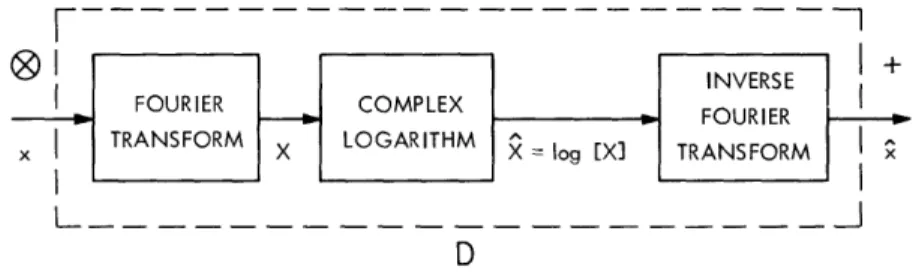
Equations 5 and 6 suggest that under an appropriate definition of the logarithm, we might define the system D to be the system whose output Fourier transform is the complex logarithm of the transform of the input; that is,
X = log [X].
Furthermore, this suggests the method of realizing the transformation D shown in Fig. 3.
Thus homomorphic deconvolution is based on transforming a convolution into a sum and then using a linear system to separate the additive components. The result is then transformed back to the original input space.
-ue
-a
FOURIER COMPLEX INES
FOURIER
I TRANSFORM X LOGARITHM = [XI TRANSFORMg
D
Fig. 3. Formal realization of the characteristic system for homomorphic deconvolution.
We have chosen for investigation, as examples of the application of homomorphic deconvolution, the class of signals that can be represented as a convolution in which one of the components is an impulse train. As an example of this class consider
x(t) = s(t) + as(t-t) = [uo(t)+auo(t-to)] ® s(t). The Fourier transform of this equation is
X(W) S(c)[ l+ae
The complex logarithm is formally
X(W) = log [S(c)] + log ( + a e °).
We note that the second term in this expression is periodic in with a repetition rate proportional to to.
Suppose we view log [X(X)] as a waveform to be filtered with a linear system. We note that if the spectra of log [S(c)] and log (1 + e
)
do not overlap, the separation of the two components is relatively easy. Alternatively, we require that the term log (+a e °) vary rapidly, compared with the variations in log [S(w)]. Thus we see that the transformation D allows us to transform a convolution of waveforms into a sum that, under appropriate conditions, can be separated by a linear system. This allows one who is familiar with linear system theory to apply all of his experience and intuition to this technique of deconvolution simply by focusing his attention on the log of the Fourier transform and interchanging the roles of time and frequency.1.2 THE CEPSTRUM
Independently of Oppenheim's formulation of the theory of homomorphic systems and 10
our subsequent work, Bogert, Healy, and Tukey0 recognized that the logarithm of the power spectrum (the Fourier transform of the autocorrelation function) for a signal con-taining an echo should have a periodic component whose repetition rate is related to the
echo delay. Thus the power spectrum of the logarithm of the power spectrum should exhibit a peak at the echo delay time. This function was called the cepstrum" by trans-posing some letters of the word "spectrum." Noll1 2 has traced the evolution of cepstral
analysis and also discussed various definitions of the cepstrum which have been employed. Although cepstral methods have been developed from an empirical point of view, we can see that the cepstrum is clearly related to homomorphic deconvolution. The basic difference is that we shall employ a Fourier transform (magnitude and phase), rather than the power or the energy spectrum. We do this because we are concerned with the more general problem of recovery of signals as opposed to detection of echoes. To emphasize this distinction, we shall refer to the output of the characteristic sys-tem D as the complex cepstrum.
II. ANALYSIS OF DISCRETE-TIME HOMOMORPHIC DECONVOLUTION
We have introduced the concept of systems that obey a generalized principle of super-position in which addition is replaced by convolution. Since it appears, at present, that such systems can be most easily realized digitally, we shall be concerned henceforth only with discrete-time systems of this class. Thus our signal vectors are sequences of numbers, and convolution is defined as
00
x(n) =
>
xl(k) x2(n-k). (7)k= -oo
The canonic form for discrete-time homomorphic systems is shown in Fig. 4, where x is the input sequence, and is the complex cepstrum. The system D characterizes all systems of this class. Therefore we shall begin our study of such systems with a study of the system D, and then consider the choice of the linear system L.
@1
~~~+
…~~~~~~~~~~~~~~~~~~~~~~~~~
+ + + 1 xX D x L DL~~~~~~~
~~-
I
__
H,
I
Fig. 4. Canonic form for discrete-time homomorphic deconvolution.
The properties of the transformation D can best be analyzed by considering the z-transforms of x and x.23 26 If x is a convolution,
X=X 1 x
then
X(z) = Xl(z) X2(z). (8)
(Note that ) denotes discrete-time convolution as in Eq. 7.) We require that if x is a convolution as in Eq. 7, then
A A A
x=x + x .
Thus the z-transform of x must be of the form
X(z) = X1(z) + X2(z) (9)
If we compare (8) and (9), we see that the requirement is that the system D effectively
7
transform a product of z-transforms into a sum of corresponding z-transforms. We shall show that, under appropriate definition of the complex logarithm,
log [X1(z)X2(z) ] = log [X1(z) ] + log [X2(z)].
Thus we are led to define the system D as one for which the z-transform of the output is the complex logarithm of the z-transform of the input. That is,
00oo
-n
X(z) = x (n) z = log [X(z)]. (10)
n=-oco
Since log [X(z)] must be a z-transform, it must have the properties of a z-transform. In particular, we must be able to define a region (actually a Riemann surface) in which log [X(z)] is single-valued and analytic and possesses a Laurent series expansion. Thus before proceeding to the actual definition and discussion of the realization of the sys-tem D, it is first appropriate to review some of the properties of the complex logarithm.
2. 1 COMPLEX LOGARITHM
The function X(z) can be expressed as X(z) = 1X(z) j ej arg [X(z)]
The logarithm of X(z) is defined as
log X(z)] = log X(z) + j arg [X(z)]. (11)
since ej 2 wq = 1 for any positive or negative integer q, it is clear that we may always write arg [X(z)] as
arg [X(z)] = ARG [X(z)] ± j2irq, where q = 0, 1, 2, .. , and
-7r < ARG [X(z)] < t.
Therefore log [X(z)] may be expressed as
log [X(z)] = log X(z) + j ARG [X(z)] j2Trq. (12)
That is, the complex logarithm is multivalued, with infinitely many possible values. The principal value of log [X(z)] is defined as the value of Eq. 12 when q = 0, and ARG [X(z)] is called the principal value of arg [X(z)]. (Henceforth, the principal value of an angle will be denoted by capital letters.)
The transformation D must be unique. Therefore the logarithm must be so defined
that there is no ambiguity with respect to its imaginary part. Furthermore, we require that log [X(z)] be analytic in some annular region of the z plane because the values of the complex cepstrum x are defined as
(13) x(n) = 21 A log [X(z)] 1 dz.
In Eq. 13, C is a circular contour specified by z = e + j -T < < 7 r,
where e is the radius of the circle. In Eq. 13 it is assumed that log [X(z)] has a Laurent series expansion as in (10). Thus we must insure that log [X(eU+JW)] is analytic in an annular region containing the circle with radius e. This region is appropriately called the region of convergence of log [X(z)] or of X(z).
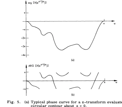
In general, the principal value of the phase, ARG [X(e+jWo)] will be a discontinuous function of . In fact, ARG [X(e+jW)] will be discontinuous for values of for which
arg [X(ea+Jo)] = nr, n= ±1,+3,+5,.. .
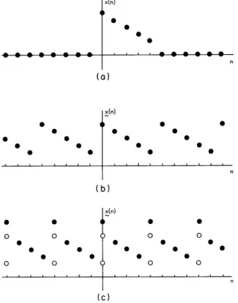
A typical example of a phase curve and its corresponding principal value is shown in Fig. 5. If the principal value of the phase is used in defining the complex logarithm,
(a) _.1.:.,
Fig. 5. (a) Typical phase curve for a z-transform evaluated on a circular contour about z = 0.
(b) The principal value of the phase curve in (a).
9
: - g
its derivative does not exist at the points of discontinuity of ARG [X(eU+Jj°)]. Therefore the function log [X(ec+Jw)] would fail to be analytic at these points. Because log [X(z)] must be analytic on the contour C, we must eliminate such singular behavior by com-puting a phase curve with no discontinuities.
We also recall that if X(z) = Xl(z) X2(z),
then we require that
log [X(z)] = log [X1(z)] + log [X2(z)],
on the contour C. If we write
X1 (z) = X(z)I ej arg [X(z)]
and
X2(z) = 1X2(z)l ej arg [X(z)]
then we require that
log X(z) = log I X1(z) + log I X2(z) (14)
and
arg [X(z)] = arg [X1(z)] + arg [X2(z)], (15)
where z = e a+ j ' and - < < Tr. Since log X(z) | is simply the logarithm of a positive real number, (14) will be satisfied whenever X1(z) and X2(z) are nonzero and finite.
With respect to the phase angles, we can write
arg [X(z)] = ARG [X(z)] j2Trq (16a)
arg [Xl(z)] = ARG [Xl(z)] j2wql (16b)
arg [X2(z)] = ARG [X2(z)] i± j2wq2, (16c)
where q, q, and q2 are integers. Clearly, (15) will hold only if we choose the
appro-priate value for arg [X(z)]. For example, suppose that we choose the principal value for all angles. It can be shown that, in general,
ARG [X(z)] ARG [Xl(z)] + ARG [X2(z)].
One way of insuring that (15) will always hold is to assume that all angles are computed so that they are continuous functions of as z varies along the contour C specified by z = e+j. This implies that for each value of , we have chosen the proper values for
10
---q, ---q, and q2 in Eqs. 16 so that all angles are continuous functions of . In the actual
computation we only compute arg [X(z)], so the proper choice of q1 and q2 is implicit
in the proper choice of q. Thus requiring that the phase curve be continuous also implies that Eq. 15 is satisfied.
Two other restrictions on the form of arg [X(z)] result from considerations that do not have to do with the logarithmic operation. If we require that x(n) be real when x(n) is real, the real part of (e +j) must be an even function of and the imaginary part of X(e j ) must be an odd function of . Since X(e*+J')
J
is even for real x(n), so isRe [X(e7+jco)] = log X(e*+Jw)I.
The requirement on the imaginary part implies that we must define arg [X(ea+Jo)] = -arg [X(e*- j o ) ] .
A final condition is required because log [X(z)] is to be the z-transform of the sequence x; log [X(eU+jo)] must be periodic in X with period 2. That is,
log IX(ea+Jw)I = log I X(ea j+ j 2 " k ) and
arg [X(ec+J)] = arg [X(ea+Jw±j21Tk)]
where k = 0, 1, 2 .... This periodicity and the even and odd symmetry properties
imply that log X(e'+Jco) has even symmetry about 0, ±r, 2'r .., and likewise
arg [X(ea+Jw )] has odd symmetry about X = 0, iTr, 2....
To summarize, the conditions that are imposed on Im [X(z)] = arg [X(z)]
are the following.
(C1) arg [X(z)] is a continuous function of X for z e+. (C2) arg [X(z)] is an odd function of X for z = e+® .
(C3) arg [X(z)] is periodic in , with period 2 for z = e + j o'.
Conditions similar to (C2) and (C3) apply to log X(z) and follow automatically from the definition of the logarithm of a real number and the symmetry properties of the mag-nitude of a z-transform. These conditions are the following.
(C5) log
IX(z)
is an even function of for z = e + j w.(C6) log
IX(z)
is periodic in o, with period 2 for z = e + j° ..11
--2. 2 REALIZATIONS FOR THE SYSTEMS D AND D
We have seen that if special care is taken in defining the complex logarithm, the logarithm of a product of z-transforms is the sum of the logarithms. Furthermore, under these conditions, log [X(z)] can also be thought of as the z-transform of the
D
TWO-SIDED log I I I R
I v_ z-TRANSFORM
x X(z) () = log [X(z)] x
D
Fig. 6. Realization of the characteristic system for homomorphic deconvolution using z-transforms.
complex cepstrum. Thus, one realization of the system D is that shown in Fig. 6. The complex cepstrum is seen to be the result of the equations
00
X(z) = x(n) z -n (17a)
n= -oo
X(z) = log [X(z)] (17b)
x(n) = 2-j log [X()]zn 1 dz, (17c)
where the closed contour C lies in a region in which log [X(z)] has been defined as single-valued and analytic.
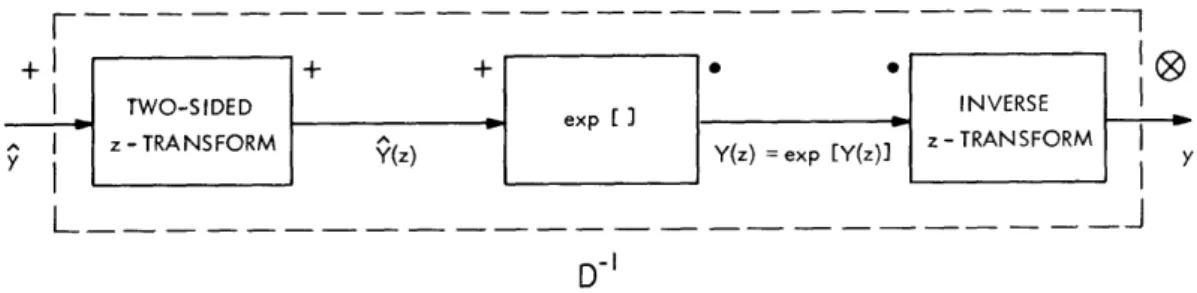
+
l
+·-kl eJ INVERSE
TWO-SIDED ex INVRS
z
z-TRANSFORM (z Y(z) ex [(z) z-TRANSFORM
y I Y(Z)
~~~~~~~~~~Y(z)
=exp [Yz)D-l
L~~~~~~~~~~~~~~~~~~~~~~~~~~~~~~
Fig. 7. Realization of the inverse characteristic system for homomorphic deconvolution using the z-transform.
Similarly the inverse of the system D is shown in Fig. 7. Thus, we obtain for the output of D the equations
00oo
Y(z) = y(n) z (18a)
n=-oo
Y(z) = exp[Y(z)] (1 8b)
y (n) = 21j Y(z) zn-1 dz. (18c)
In (18c) the contour C' must be a closed contour in the region of convergence of the input z-transform X(z). This is required because if the linear system is the identity system, we require that the over-all system be the identity system; that is, if
y(n) = x(n), then
y(n) = x(n).
2.3 INTEGRAL RELATIONS FOR THE COMPLEX CEPSTRUM
We have shown that the complex cepstrum can be obtained from the set of equations
00
X(z) = x(n) z-n (19a)
n= -oo
X(z) = log [X(z)] = log X(z) + j arg [X(z)] (1 9b)
A 1 -~~ A n-i
x(n) = 2j X (z) zn 1 dz. (19c)
These equations constitute a definition of the system D and also lead to a computational realization. We shall consider Eq. 19c and show how it may be used in studying the prop-erties of the system D.
We have seen that the circular contour C must lie in the region of convergence of
A
X(z). In using these equations for computation, part of the definition of the system D
A
is the choice of the region of convergence of X(z). In general, the two-sided transforms
A
~~~~~~~~~~~~~~~~~23
26X(z) and X(z) have regions of convergence which are annular regions of the z plane. 3 26 For example, we shall usually denote the region of convergence by a relation of the form
R+ <
zl
<R_.By definition, these regions can contain no singularities of the z-transforms. The regions of convergence may, however, contain zeros of the z-transforms, and we shall see that
A A
these cases require special handling. Since X(z) is the complex logarithm of X(z), X(z) will have singularities at all of the singularities and at all of the zeros of X(z). Similarly,
13
X(z) will have zeros at all of the ones (X(z) = e ) of X(z). Therefore we see that the region of convergence of X(z) can be the same as the region of convergence of X(z) only if X(z) has no zeros in its region of convergence. On the other hand, it should be clear that we are free to choose any annular region that does not contain singularities or zeros of X(z) as the region of convergence of X(z).
The choice of the region of convergence for X(z) is based primarily on computational considerations, and at least two different choices have been found useful. In any case, it should be clear that for a given input sequence x, it is possible to obtain many dif-ferent output sequences x depending on the region of convergence that is chosen for
A
X(z). This does not mean that the output is not unique because the choice of the contour C
A
(and therefore the choice of the region of convergence of X(z)) is part of the definition of the characteristic system D. Once this contour is fixed, the output is uniquely deter-. mined.
Let us temporarily leave the contour C unspecified and obtain a more useful expres-sion for x(n). Using Eqs. 19b and 19c, we obtain
1 ~C z~n-1
x(n) = log [X(z)]n 1 dz. (20)
If we note that the contour C is specified by z = e+j, with -rr < < aT, we can write (20)
1 j~~~~~~nwn
X(n) = Tr log [X(e+J)] ean ei n de. (21)
We shall proceed to integrate (21) by parts under the assumption that log [X(eU+Jw)] is a single-valued periodic function of which is everywhere continuous. We shall find that this assumption is somewhat restrictive, but we shall also show how the results derived here apply to more general circumstances.
If we integrate (21) by parts, we obtain, for n # 0,
x (n) =
~[log
[lg[(ea+i(o)]ei(Aon][l
-1 -e'lo[X(eg+)]2
1QTd'tvi+C~~) e
ne
ij~c ndo.
27Tjn - 2jn -e
Because both log [X(ea+Jco)] and eijn are periodic with period 2r, the first term in the expression above vanishes. Since we have assumed that log [X(e+Jiw)] is continuous everywhere, we obtain
o d f +'
(n) 2rjn + en ejn d. (22)
~n ld,, X(en
Since the logarithmic derivative is also analytic in the region of convergence of X(z) we may write (22)
x(n)- 2,jn zX'(z) 1 dz, (23) where the prime indicates differentiation with respect to z. The contour C is, of
A~~~~~~
course, still in the region of convergence of X(z).
The value of x at n = 0 is obtained directly from Eq. 21; that is,
x(0) = 2r i- log [X(ea+Jo)] do.
1T
Since arg [X(e"+jo)] is an odd function of wo and log X(ea+jo) is an even function of ,
x(0) = 2f ,9 log X(e+J )I d. (24)
-1T
Thus as an alternative to Eqs. 19 for analysis, and possibly for computational pur-poses, we have Eqs. 23 and 24, under the assumption that X(e + jw) is a single-valued
and continuous function of for all a. We shall see that this condition must be relaxed in order to include most situations of interest. (This will be done in section 2. 9.)
2.4 "TIME-DOMAIN" EXPRESSIONS FOR THE COMPLEX CEPSTRUM
A
The expressions just derived gave the complex cepstrum x explicitly in terms of the z-transform of x. Equation 23 may be used to obtain an implicit expression in terms of x(n) and x(n) which, in certain cases, reduces to a recursion formula.
This implicit relation may be derived as follows. If we assume that log [X(e'+Jw)] id continuous for all , we can write
X' (z)
X' (z) =
X(z)
Rearranging this expression, we obtain
zX'(z) = zX'(z) X(z). (25) Since oo 00~
~
-X'(z) = z- 1 ~ -nx(n) z n n=-oowe see that the inverse z-transform of (25) is
00
nx(n) = I k2(k) x(n-k). (26)
k= -oo
15
-There are several special cases of (26) that are worthy of special consideration. Case 1: x(n) = 0 for n < 0, and x(0) 0.
In this case we can write n
nx(n) = kx(k) x(n-k),
k=-oo which can be written as
n-1
x(n) =-) n # 0. (27)
x(0) n k=-ox(0)
Thus we see that x(n) depends on all values of x and the values of x for k < n.
Case 2: Suppose that x(0) 0 and x(n) = 0 for n < 0. If we further assume that x(n) = 0 for n < 0, we obtain from Eq. 27
x(n) n-l x(n-k)
x (n) (.2 jk (k) n >0. (28)
x(0) k=0 x(0)
The value of x(0) for sequences of this type can be shown to be (see section 2. 5)
2(0) = log x(0). (29)
Requiring that £(n) = 0 for n<0 is equivalent to choosing the contour C in (23) so as to enclose all of the poles and zeros of X(z). If X(z) has poles or zeros outside the unit circle, it can be shown2 3 that x(n) will be unbounded for large n, since we are effec-tively choosing the region of convergence to be outside of all of the poles and zeros of X(z). This will not be the case, however, if X(z) has all of its poles and zeros inside the unit circle.
Thus when X(z) has all of its poles and zeros inside the unit circle, (n) satisfies a recursion relation that could be used in actually computing x(n). (Discussion of the util-ity of this expression is reserved for Section III.)
Finally, we observe that Eqs. 28 and 29 provide a way of obtaining x from x, that is, a recursive relation for the inverse characteristic system. By rearranging Eqs. 28 and 29, we obtain
x(0) = e(0) (30a)
n-i1
x(n) = x(n) x(0) + ( (k) x(n-k) n> 0. (30b)
k=0
Equations 30 represent a realization of the inverse characteristic system for sequences whose z-transforms have no poles and zeros outside the unit circle.
Case 3: Suppose that x(0) 0, (n) = 0 for n < 0, andx(n) = 0 for n< 0 andn > M. In this case, Eqs. 28 and 29 take the form
x(0) = log x(0) (31a) x(n) n- kn x(n-k) £(n) = - - I ( S) ^x(k) 0 < n-< M (31 lb) x(0) k=0 x(0) x(n) n-l x(n-k) =- -_ _ X (-) x(k) n > M. (31c) x(0) k=n-M x(0)
Case 4: Let x(n) = x(n) = 0 for n > 0 andx(0) 0.
These assumptions are equivalent to taking the contour C in (23) to be inside all of the poles and zeros of X(z). Thus for a stable sequence x, we require that all of the poles and zeros be outside the unit circle.2 1 Using Eq. 26, we arrive at
x(0) = log x(0) (32a)
~()x(n) 0 k
(n) n) - n) x(k) x(n-k) n < 0. (32b)
x(0) k=n+ 1
2. 5 COMPLEX CEPSTRUM FOR SEQUENCES WITH RATIONAL z-TRANSFORMS
In actual computations, we are always restricted to sequences of finite length and hence to z-transforms that are simply polynomials in z 1 Thus it is not a significant restriction if we consider z-transforms of the form
m. 1 (1~ m0 II I -akz ) (1-bkZ) X(z) = A , (33) Pi p0 II (-C kZ-') II ( -dkz) k= 1 k=
where A is a positive-real constant, and the ak, bk, ck and dk are nonzero complex numbers whose magnitudes are less than one. If x is a real sequence, then the ak, bk,
ck and dk occur in complex conjugate pairs. Careful examination of Eq. 33 shows that there are mi zeros and Pi poles inside the unit circle, and m0 zeros and po0 poles
out-side the unit circle. Clearly, (33) is not the most general rational z-transform, since r
A could be negative and in general we must include a factor of the form z to account for all shifted versions of the sequence x. Since our method in computation will be to
deal with these issues separately, we shall defer discussion of these points.
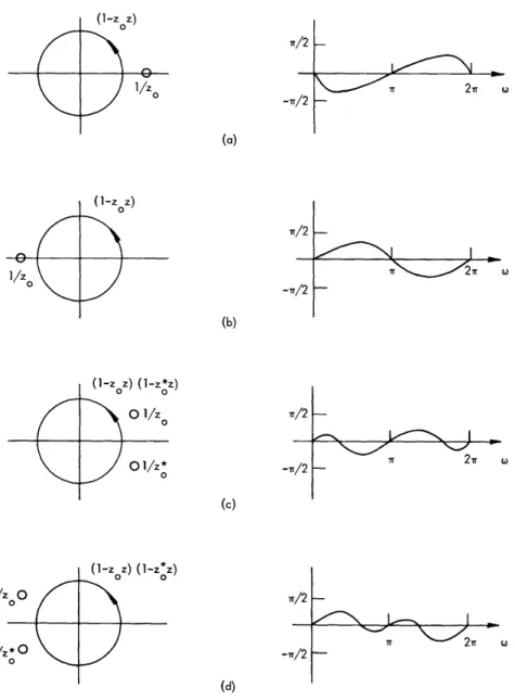
(1-z z- ) lr/2 (a) (b) (l-zOz ) (-z*z ) 0A 0
.
0
(c) (-zo- 1) (-z*z-I) r/2 (2) (d) -i/2 - 2r~I
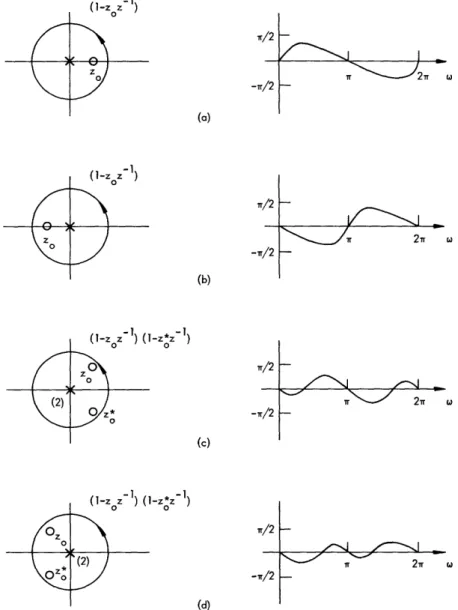
IT 2rrFig. 8. Phase curves for zeros inside the unit circle.
18 (2) oz IQZ £ (d 2n tI /2
zll-i - -_< _11/z O 1/z*0 0
~
(1-z Z) </2 l / (a) (1-z z) 1 \ 1Z Z r/2 -./2 (b) 0 0/ t~z)~ -oZ 1Tr/2 --r/2 2r 0o 1/ 0 (C) (1-ZoZ) (-Zoz) -r/2 -</2 (d)Fig. 9. Phase curves for zeros outside the unit circle.
19 2r t ,:~~L-1 I
-a
i
,, -2 .---
·---
·---
·- --
- ·--
· ---
·----
·--
_~~ . c-We have shown that the phase curve must be a continuous function of . Since arg [X(e°+Jw)] will be the sum of the arguments of each multiplicative factor in Eq. 33, it is helpful to consider the contributions from each of these factors. Figures 8 and 9 show the typical pole-zero plots and one period of phase curves when z = e for each type of numerator factor in Eq. 33. The corresponding denominator factors produce phase curves that are the same except for sign. In all cases, the peak value of these phase curves is less than or equal to Tr/2. The value r/2 is attained only when the zeros
(or poles) lie on the unit circle. If the zeros (or poles) are on the unit circle, the phase curves become discontinuous. We also observe from Figs. 8 and 9 that all of the phase curves of these factors are zero at = 0, ±r, ±2r, ....
Since the total phase curve for Eq. 33 is the sum of the phase curves of each factor, the total phase curve will be zero at c = 0, , +2r, .... Furthermore, it is clear that arg [X(e +Jco)] will in general be greater in magnitude than 1rT. Therefore in computing the phase, we must use an algorithm that enables us to determine the correct phase curve, that is, one without discontinuities.
One such algorithm computes the principal value of the phase and then determines the correct multiple of 2r to add to or subtract from the principal value for each value of . This algorithm is discussed in Section III.
We are also interested in log X(eU+J) , since this is the real part of the complex logarithm. Since the magnitude is an even function of , it will have the same general form for poles and zeros both inside and outside the unit circle. Let us consider a fac-tor such as - zz 1 )for z = ei, and z = |zo e °. The magnitude of such a factor is
l-zo
e-J'
= 1+ zo
2I
2zo cos(-]
0)
Taking the logarithm, we obtain
log I -z e I = log + Iz 2-21zo cos (w-O).
0 Z~~~~~~~csco,)
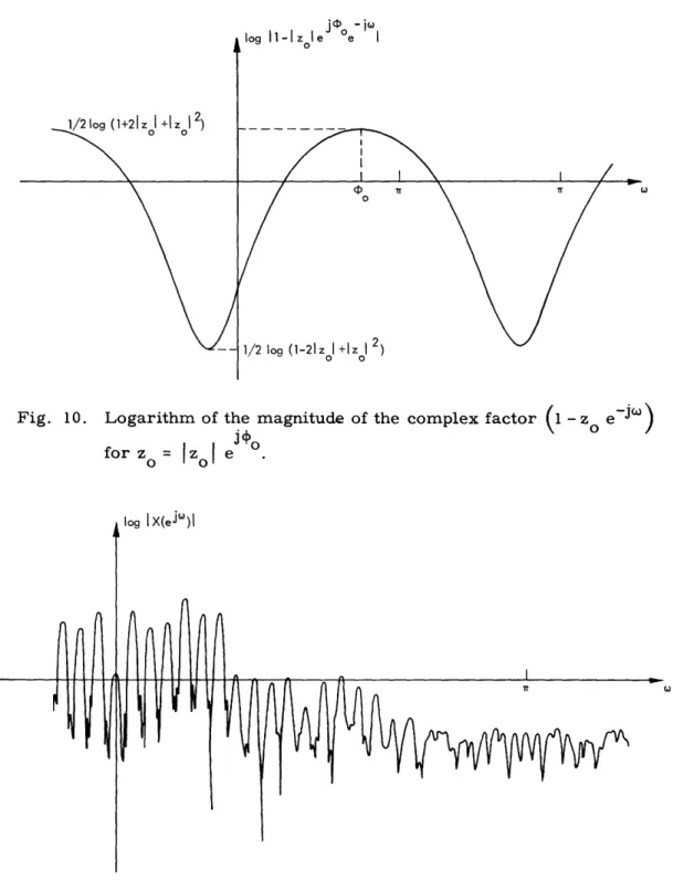
This function is sketched in Fig. 10. We note that it is periodic with period 2. The maximum positive value is - log (1 +2|z + zO12) which approaches log (2) as zo
approaches 1. Similarly, the most negative value is 2 log (1 -21 zo + [zo 2) which
approaches log (0) or -o as Izo[ approaches 1.
Since log I X(eJc) I is the sum of terms such as this (with negative signs for denom-inator factors), we would expect that log X(eJWo){ would have an appearance similar to that of Fig. 10, except that in general there will be peaks corresponding to each of the poles and zeros of X(eJW). A typical example of log X(e j o ) is shown in Fig. 11.
We have seen that z-transforms having the form of Eq. 33 satisfy the requirement that log [X(ea+Jw )] be continuous everywhere. Thus we may employ Eq. 23 to evaluate the complex cepstrum. The integrand zX'(z)/X(z), in this case, is
1/2 log (1+21 zol +1zl 2) Ij -; 1_ I 1 _I ! I ( IT 0 log (1-21 z + zI 2) 0 0
Fig. 10. Logarithm of the magnitude of the complex factor (1 - z e for z0 = z e 0 .
I I t ( I
log IAte- )I
F
Fig. 11. Typical curve for the logarithm of the magnitude of the z-transform of a finite-length sequence.
21
RRR
- - -_ _
m. X' (z) 1 X(z) k= x(z) L= -1 akz -1 1 - akz m o bk * ,1 - bkZ-k= 1 Pi k= 1 -1 ckZ 1 - CkZ PO + dkZ k1 dkZ k= (34) Since -1 zX'(z) x(n) = zTjn X(z) dz,
we see that if we desire a stable sequence (one whose values approach zero for large n), we must choose the region of convergence to include the unit circle. Each factor in (34) is the z-transform of an exponential sequence. Therefore, if the contour is taken as the unit circle, (n) is given by
n ck _ n -n k _ n m. 1 n k=l m o dn k An k= (35a) n -1. (35b)
The value of x(O) is obtained from Eq. 24 with = 0. Therefore
-rr
log X(eJo) d.
Each factor of X(eA) Ihas the form
1 -a e:Jw@ = 1 + aJ2 - 21a I cos (:F arg[a]),
and it can be shown that
21 log (1 + I a 2- 2 la cos (cow:F arg [a])) dco = 0, -Tr
if l al < 1. Therefore we see that x(o) = 2 1
Y
-_IT Equations z-transform. is clear from log A do = log A. (36)35 and 36 express (n) in terms of the poles and zeros of the rational They also illustrate an important property of the complex cepstrum. It Eqs. 35 that 22 Pi x(n) = k= 1 Po
k=
1
k= 1|x(n)I B an
[nl
n #0,
where B is a positive constant and a is the magnitude of the pole or zero that is closest to the unit circle.
In many simple cases, it is not necessary or desirable to use the integral formulas for purposes of analysis. This is particularly true when the z-transform is a rational function. In this case a power-series expansion of log [X(z)] is usually more convenient.
Under the assumptions that log [X(z)] is defined to be single-valued and analytic in the region of convergence, and that X(z) has the form of Eq. 33, we may write
m.
1
log [X(z)]= log A + log(1-akz -1) k= 1
mo Pi Po
+ log (-bkz) - ; log (1-ckz -1) - log (-dkz).
k k= 1 k=1 k=
Since we define X(z) as a z-transform, it must be true that
00
(37)
^
~~~~~~~-n
X(z) = log [X(z)] = x(n) z . (38)
n= -o
Thus we immediately see that x(0) = log A.
If we effectively take the contour C to be the unit circle, then each of the remaining terms in (37) can be expanded in a Laurent series about z = 0. For example, we can write
o0 n ak -n = -Z n n= 1 co n -log (ckZ1) = k z- n n= 1 log (l-bkz) -log (-dkz) -1 b-n = bk -n =
~
nZ n n=-oo - 1dn = _ Y _ -n = n z n= -oo for Iz > akI for Jz > cki forIz
< bkl forIz
< dkl'. 23 log (1-akz ) ---·II- --~-
~
-- --- I-Therefore if we add these convergent series and collect the coefficients of z n, we can
determine x(n). In general, we see that (n) can be written
x(0) = log A (3 9a) p. m. Pi n mi n x (n) = E n a 1 (39b) k= 1 k= m p _o -n o -n = b n k. <k (39c) n n k=I k=1
Equations 39 agree with Eqs. 35 and 36, as we would expect. The real value of the power-series approach is best illustrated by our use of it in discussing echo removal applications in Section V.
2.6 MINIMUM-PHASE AND MAXIMUM-PHASE SEQUENCES
We have considered a realization of the system D which was based on the z-transform. In some cases it is possible to take advantage of the properties of the z-transform to obtain simplified results. For example, we have seen (section 2. 4) that under certain conditions, (n) obeys a recursion formula. We shall now consider these cases in detail and present an alternative computation scheme.
A minimum-phase sequence is defined as a sequence whose z-transform has no poles or zeros outside the unit circle. Furthermore, the region of convergence for the z-transform includes the unit circle. For rational z-transforms, X(z) is of the form
m.1 (1) I ( 1 ) X(z) = A k Pi I (1 -ck z - ) k=
where the ak and ck are complex numbers whose magnitudes are less than one, and the region of convergence is specified by
Z
>maxIckl.
k
Such sequences have the properties
x(n) = 0 n < 0 (40a)
x(O) • 0 (40b)
o00
I x(n) <
oo.
n=0
We have shown that the complex cepstrum of such a sequence has the properties x(n) = 0 A x(0) = log x(0) 00 E |x(n) < o. n=O0 n<0 (40c) (41a) (4 b) (41c)
Since Eqs. 40 and 41 are necessary and sufficient conditions, these equations could be taken as the definition of a minimum-phase sequence.
An entirely analogous situation is called maximum-phase. In this case, X(z) has all poles and zeros outside of the unit circle, and the region of convergence includes the unit circle. In this case, x has the properties
x(n) = 0 x(O) n>0 (42a) (42b) (42c) 0 Jx(n) < oo. n=-oo
Similarly, the complex cepstrum has the properties
x(O) = n>0 (43a) (43b) (43c) x(0) = log x(0) 0
Z
Ix(n) I
<
.
n= -ooFor rational z-transforms, X(z) has the form m o B II (-bkz) X(z) = k=1 Po II ( -dkZ) k= 1
where the bk and dk are all less than one in magnitude, and the region of convergence is
25
Jz <min dklI. k
In general, there may be poles and/or zeros on the unit circle. These cases will be formally excluded from either class; however, we shall see (section 2. 7) that it is possible to move such poles and zeros inside or outside the unit circle by exponential weighting of the sequence.
If the input sequence is known to be minimum-phase, we can obtain significant sim-plifications in our results. We have already seen that the characteristic system D and its inverse can be realized through a recursion formula. We now wish to show that the properties of minimum-phase sequences allow other simplifications in the computation of the complex cepstrum.
Let us introduce some definitions. We define the even part of a sequence to be the sequence whose values are
x(n) + x(-n)
Ev [x(n)] = 2 (44)
The sequence Ev [x(n)] is seen to have even symmetry; that is, Ev [x(n)] = Ev [x(-n)].
Similarly, we define the odd part of a sequence as x(n) - x(-n)
Odd x(n)] = 2 ' (45)
which has odd symmetry; that is, Odd [x(n)] -Odd [x(-n)].
It can be shown that if x is a real sequence and X(eJW) = Xr(eJW) + jXi(eJ°),
then Xr(e ) is the transform of Ev [x(n)] and similarly, jXi (e) is the transform of Odd [x(n)].
Let us assume that x(n) = 0 for n < 0. In this case we can see from Eq. 44 that x(n) = 2 Ev [x(n)] n > 0
= Ev [x(n)] n = 0
=0 n<0.
That is, knowledge of the even part of a sequence that is zero for n < 0 is sufficient to
determine the entire sequence.
These properties represent a real part sufficiency theorem for z-transforms of
sequences that are zero for n < 0. For example, suppose we are given the real part Xr(eJ ) of the transform of a sequence x. Since Xr(eJ&)) is the transform of the even part of the sequence, we can determine Ev [x(n)] from Xr(eJl°). If x(n) = 0 for n < 0, we can determine the sequence x and therefore X(eJ°). Thus knowledge of Xr(eJ ) is suf-ficient to completely determine X(eJ').
Similar relations hold between the logarithm of the magnitude and the phase of a z-transform, but under more restricted conditions. Rather than focus our attention on relations between the magnitude and phase, let us consider the complex cepstrum first and return to this question eventually. If x(n) = 0 for n < 0, we can apply the previous results to the complex cepstrum to obtain
x(n) = 2 Ev [(n)] n > 0 (46a)
= Ev ['(n)] n = 0 (46b)
= 0 n < 0. (46c)
A
Since the real part of X(eJ ) is just
Xr(ei) = log X(eJ')|,
we see that
Ev [(n)] = log X(eJC) ej d. -Tr
Thus, if x(n) = 0 for n < 0, we only need to compute
Xr(ejO) = log X(ej c')I,
and we do not need to compute the phase.
If we wish to obtain the original sequence from log fX(eJ°) |, we can do so by first computing Ev [(n)], then x by using Eqs. 46, and then obtain the original sequence by using the inverse characteristic system to compute x. Since the condition x(n) = 0 for n < 0 has been shown to be equivalent to the condition that x be minimum-phase, we see that for minimum-phase sequences, the complex cepstrum can be computed from
00 X(ej c') = x(n) e- jwn (47) n=O0 Ev [xn) = r log X(eJ°) e n do (48) -Tr x(n) = Ev [x(n)] u(n), (49) 27 .- I
where
u(n) = 2 n>O
=1 n=
=0 n < 0.
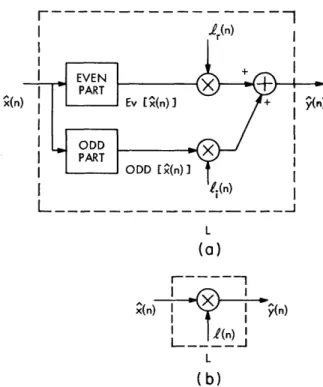
Thus the characteristic system D for minimum-phase sequences can be realized as j).
shown in Fig. 12, where "Fourier Transform" means X(e ).
Clearly, the discussion above also indicates a unique relation between log X(e3j)I
Fig. 12. A realization of the characteristic system D for minimum phase sequences.
and arg [X(eJW)]. In fact, the operations illustrated in Fig. 12 are equivalent to using the Hilbert transform 4 to obtain the proper phase curve for log X(ejW) I when X(ejW)° is minimum-phase.
As an example of the use of this result, let us consider the minimum-phase sequence x(n) = a
=0
n 0
n < 0.
The z-transform of this sequence is 1
X(z) = 1
1 - az
for lzl > lal,
and
log X(ejf)l = -Ilog (l+a2-2acoso).
Therefore the even part of the complex cepstrum is
Ev [(n)] = - log (+a 2-2a cos ) ei dc -1T
which can be written
Ev [x(n) = -
'So'
log (+a -2acosw) cos con d. 28At this point, let us note two useful equations which can be found in Carslaw.21
2~~~~~ g 0 log (+a -2acoswa) d = 0
= log a
log
a 22a
$ log (1+a -2acosa) cos an dc =
-0 a l
alnJ
Inf 1 (50) laI < 1 =_a~
JnI
- - T a- nIn!
These equations hold for n an integer. Ev [(n)] = 0
1 a n
' Inj
We can use (50) and (51) to show that n= 0
n 0.
Therefore we see that n
x(n) = 2 Ev [x(n)] = a n > 0
n
=0 n < 0.
In conclusion, we wish to call attention to an interesting representation of the input sequence, and an interesting result for finite-length sequences. It is clear from the properties of minimum-phase and maximum-phase sequences that every sequence x may be expressed as xmin max' where x .min (n) = (n) mi(n) Xmax(n) = 2(n) n >0 n < 0.
For rational z-transforms, this is equivalent to X(z) = Xmin(Z) Xmax(z), where 29 and (51)
1111
11
1_11(1111_-
-l- ., l ·m. I - 1 ) Xmin(Z) = Xmax(Z) = K- I Pi II (I-ckz - ) k= I m o II ( -bkZ) k=l 1 Po II (1 -dkZ) k=l
The results given here have particular significance for finite-length sequences. Suppose that X(z) has the form
m. 1 -I X(z) = A II (l-akz k= m
)
n
k=l (1 -bkz), where the ak and bk are all less than oneXmin(n) 0 = 0O Xmax(n) 0 in magnitude. 0 n m. 1 elsewhere -m n O o = 0 elsewhere.
From Eqs. 30 and 32, we obtain the relations
xmi mmn. (n) = ee ( ) = x(n) x(O) + n-1 k=O (-) \n x(k) Xmiminn(n-k) Xmax(n) = 1 n=0 0 = x(n) + (-) x(k) Xmax(n-k) k=n+ 1 n < 0.
We see, therefore, that only mo + mi + 1 values of the complex cepstrum are required to completely determine the m + mi + 1 values of the sequence x. This
30 and Clearly, n >0 -
I
__
A
result implies that even though x is of infinite duration, only a number of samples of x equal to the length of the input sequence x is required to completely determine the sequence x from the complex cepstrum.
2.7 EXPONENTIAL WEIGHTING OF SEQUENCES
Because of the special properties of minimum-phase sequences, it is of interest to consider ways of obtaining minimum-phase sequences from nonminimum-phase
sequences. One way of doing this is to weight the nonminimum-phase sequence with a decaying exponential. By this we mean multiplication of the values of a sequence by
n
a to obtain a new sequence whose values are w(n) = anx(n).
There are two important points to consider. First, we shall consider the effect of expo-nential weighting on a convolution, and then the effect on the z-transform and its region of convergence.
Suppose that x(n) is given by 00oo
x(n) = xl(k) x2(n-k).
k= -oo
For the exponentially weighted sequence, we obtain
0o 0o w(n) = an xl(k) x (n-k) = akxl(k) a kx2(n-k) k=-oo k=-oo o00 = w 1(k) w2(n-k). k= -oo
Therefore exponential weighting of a convolution of two sequences x1 and x2 is seen to
be equivalent to the convolution of the exponentially weighted sequences w1 and w2 whose
values are
wl(n) = a xl(n)
w2(n) = a w2(n).
The second interesting point is the effect of exponential weighting on the z-transform of a sequence. The z-transform of the weighted sequence w is given by
o00
W(z) = anx(n) zn = X(a lz).
n=-oo
31
Therefore we see that if X(z) has a pole or zero at z = z, then W(z) has a pole or zero at azo0. Thus if the region of convergence of X(z) is
R+ < I z <R_,
then the region of convergence of W(z) is aR+ < I z < aR_.
If we have a sequence x for which x(n) = 0 for n < 0 but is nonminimum-phase, then
the sequence can be made minimum-phase by appropriate exponential weighting We
n
simply need to multiply x(n) by a , where a is less than one and small enough to move the pole or zero with greatest magnitude inside the unit circle.
We see, then, that exponential weighting may be very useful because convolutions are preserved and it permits a more desirable pole-zero distribution. We should point out, however, that if the required value of a is too small, we shall often be troubled with rounding errors in carrying out such weighting on numbers stored in a computer.
A final point should be made. Exponential weighting clearly changes the complex cepstrum. As the value of a approaches the reciprocal of the magnitude of the pole or zero that is farthest from the origin, the complex cepstrum becomes zero for nega-tive n. If, on the other hand, a is close to 1, it will not significantly affect the complex
cepstrum, unless the z-transform of the input has poles or zeros on or close to the unit circle. Since convolutions are preserved in the weighted sequence, the complex cep-strum will always have the form
w (n) = w 1(n + w 2(n )
In general, there is not a simple relationship between wl (n) and xl (n); however, if the poles and zeros of Xl(z) are inside the unit circle, then clearly those of Wl(z) will also be inside the unit circle if
a
< 1. Thus, in this special case, if= n w (n) = a xl ( n ), then n^ w1(n) = a xl(n). w~~~~~~~~~~~~~~~~~~ (n) an x (n).
Although there may not always be such a simple relationship between w1(n) and x (n)
and w2(n) and x2(n), we do still have a way of recovering xl(n) or x2(n) if we are given
wl(n) or w2(n). This is so because
-n (n
x1(n) = a a w(n) w
x2(n) = a w2(n).
These relations are useful in practice, since they allow us to work with exponentially weighted sequences as inputs to the system D. If we desire the original sequences at the output, we can simply unweight, using the relations above. In practice, this idea is useful if we are dealing with finite-length sequences such that x(n) = 0 for n < 0 and
M.
n > M, and if we can choose a so that a is not so small as to introduce excessive rounding error.
2.8 MORE GENERAL RATIONAL z-TRANSFORMS
Let us assume that the z-transform of the input to the system D has the form
m. m 1 k ) o I_ (1-akz)II (-bkZ) r k k=l X(z) = Az k=. (52) Pi ( ) Po I (1-Ckz1 II (1-dkz) k= 1 k= 1
In all of our previous results based on rational z-transforms, we assumed that A was positive and real and r = 0. This was to insure that arg [X(z)] could be defined as single-valued and continuous. Clearly, there are many interesting sequences that do not have z-transforms of this form. For example, if we allow A to be positive or neg-ative and r 0, we can include most sequences of interest for computation. In fact, finite-length sequences have z-transforms of the form of Eq. 52, with the ck and dk all equal to zero. (Note that we have excluded zeros on the unit circle. These could be included in our discussion if we were willing to consider discontinuous phase curves and logarithmic infinities in the log magnitude. For simplicity, we shall take the point of view that zeros on the unit circle have been shifted inside by exponential weighting.) Let us now see how the results previously presented can be applied in this more general
situation.
When X(z) is actually the product of two or more z-transforms, we shall assume that each term in the product is written in the form of (52). Thus the constant A will be the product of the corresponding constants of the individual factors of X(z). For example, if
X(z) = Xl(z) X2(z),
then
A =A1 A2.
Clearly, A will be positive if A1 and A2 are both of the same sign, and A will be
nega-tive if the signs of A1 and A2 differ. That is, by consideration of the sign of A it will
only be possible to determine the sign of A1 relative to the sign of A2 . In most situations,
33
-the appropriate signs will be clear from consideration of -the source of -the signals or, in many cases, the signs will not be important.
The constant term A contributes an integer multiple of Tr to the phase. Since we can only determine whether A is positive or negative, we normally test to see if A is positive or negative before computing the phase. If A is negative, we can change the sign of X(ea+jw°) to effectively remove any contribution to the phase which is due to the sign of A. Whether A was positive or negative can be remembered if this information is of interest. The sign of A can be determined by noting that
m. 1 mo HI (I1-ak) II (1-bk) X(1) = X(ej O) = A k1 k= (53) Pi Po H (1-ck) II (I1-dk) k= 1 k=
Since the ak, bk, ck and dk are all less than one in magnitude, all of the factors in (53) are positive; therefore, the sign of A is the sign of X(1).
r.
Let us now consider the effect of the factor z in (52). Assuming that the phase is computed as specified in section 2.1, we can write formally
-- Mi m° /N I~~~~~~~I -akz-1 I I -bk Z X(z) = log [zr] + log A k= I k I (54) Pi Po H- (I Ck ) H- (I dk ) k= k= 1
Thus, the complex cepstrum x consists of a component having all of the properties that we have previously discussed and a component that is due to the term log [zr]. To see how our results are modified by this term, let us consider the phase contribution for
z = e + j . We are tempted to write log [zr] = log [ear ejwr] = or + jr.
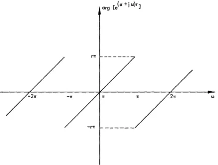
If we recall, however, that the phase angle must be periodic in (since it is the imag-inary part of a z-transform), we see that arg [e(a+j°o)r] must be defined as in Fig. 13. This factor then adds a nonanalytic component to the imaginary part of log [X(ea+j)].
Formally, the contribution to the complex cepstrum of this type of term is
= an CIT
O(n) e n
,
r log [ea+jwI] ejwJn de.-r
Performing the indicated integration shows that
0(n) = r ean cos n n 0 (55a)
n
= (Tr n =O. (55b)
34
rTT
(a
Fig. 13. Phase curve attributable to a factor zr when z = e+j .
This sequence is stable only if the contour of integration is the unit circle ( = 0). In fact, the sequence, strictly speaking, only has a discrete Fourier transform
co
a(e j ) = 0(n) e-j
wn,
n= -osince log z has no Laurent series expansion about z = 0. This situation is analogous -1
to the continuous-time function (+t 2) , which has no two-sided Laplace transform but does have a Fourier transform.
Usually, we prefer to remove the linear-phase component before computing the
complex cepstrum. This is easily done once the phase curve is computed, and
clearly its removal simply corresponds to a shift of r samples in the input sequence. This value of r can be saved and used to shift the output of D 1, if this is
appro-priate. The parameter r is very much like the sign of A, in that if X(z) is the product of X (z) and X2(z), each having the form of Eq. 52, then r = r + r2 and
it will only be possible to determine r1 and r2 from consideration of the source of
the sequence x.
Thus, the complex cepstrum of a sequence whose z-transform is of the form of (52) is normally obtained as follows. Choose the contour C to be the unit circle, and
r
find the contributions that are due to all of the factors except z , using either the power
series expansion or the integral relations. We may then simply add to this the
component (n) given by Eq. 55. For example, we could write for sequences whose
z-transforms are of the form of (52), and choosing = 0
35