DYNAMIC COUPLING OF MULTIPLE STRUCTURES
THROUGH SOIL
by
Artur Luna Pais
Diplome in Civil Engineering
Ecole Polytechnique Federale de Lausanne
Switzerland (1980)
S.M., Massachusetts Institute of Technology
(1985)
SUBMITTED TO THE DEPARTMENT OF CIVIL ENGINEERING IN PARTIAL FULFILLMENT OF THE
REQUIREMENTS FOR THE DEGREE OF
DOCTOR OF PHILOSOPHY at the
MASSACHUSETTS INSTITUTE OF TECHNOLOGY
June 1988
Copyright 0 1988 M.I.T
Signature of Author
Department of Civil Engineering
May 13, 1988 Certified by Eduardo E. Kausel Thesis Supervisor Accepted by Ole S. Madsen
chairman, Departmental Coammittee on Graduate Students
MAY '. 1Bds
LIBRARIES
ARCH I VES
-DYNAMIC COUPLING OF MULTIPLE STRUCTURES THROUGH SOIL
by Artur Luna Pais
Submitted to the Department of Civil Engineering
on May 13th, 1988, in partial fulfillment of the requirements for the Degree of Doctor of Philosophy
ABSTRACT
A two-dimensional Boundary Element formulation is developed to study dynamic problems involving several rigid foundations and tunnels embedded in a
layered halfspace. This formulation is applied in the frequency domain, and uses very efficient approximate Green's functions which can be evaluated in closed form without
the need of numerical integrations. The approximation consists in subdividing each
layer of soil into several sublayers and assuming a linear variation of the displacements across each sublayer.
The possible existence of noncausal solutions while considering nonconvex
domains is investigated with the method developed, and some comparisons with time-domain results are performed. It is found that the frequency-domain results
using the discrete Green's functions obey causality in every case.
The boundary element code is used to assess the influence of underground structures, such as a tunnel, in the seismic motion observed at the surface. A particular situation examined is that of downtown Mexico City during the earthquakes of September 1985, with focus on the effects that the underground tunnel may have
had on the motion in its vicinity. However, no significant effects were observed since
the low frequency contents of the seismic waves produced essentially translations on large structures.
An approximate procedure to evaluate the effects of the interaction between multiple foundations subjected to seismic excitations is presented. This method is relatively simple to implement and can be used in fairly general situations involving several cylindrical and rectangular foundations embedded in a halfspace. Some comparisons with more accurate methods show a good agreement, at least as far as the
qualitative effect of the interaction is concerned.
Thesis Supervisor: Dr. Eduardo Kausel
3
ACKNOVIEDGEMENTS
In first place, I would like to express my most sincere gratitude to Prof. Eduardo Kausel whose invaluable guidance and suggestions made my work in this thesis very pleasant and profitable. Prof. Kausel introduced me to the field of soil dynamics and I owe him all the expertise I have acquired. Foremost, I appreciated very much his friendship and trustful attitude which will certainly remain one of the most precious rewards of my stay at MIT.
To the many friends, students, professors and staff, who I have known during these years, especially in the Civil Engineering Department, I would like to show my special thanks. They gave me the sensation of being part of a big family with all members helping each other and contributing to the common goal of an enjoyable life during this period. I would like to mention in particular, Raymond, Tommaso, Massoud, Manuel, Luc, Fouad, Fadi, Mounir, Cemal, Jaideep, Nabil, Luis, Hayat, Otto, Thomas, ..., who despite far away geographically in a recent future, will remain in my memories for ever.
Many thanks to Otto Estorff who performed the necessary computations in the time domain used in section 3.3.2.
Finally and most of all, I would like to thank very much my dear wife Maria Eduarda who besides typing this thesis gave me all the support necessary during these years at MIT.
DEDICATION
TABLE OF CONTENTS Page ABSTRACT ... 2 ACKNOWLEDGEMENTS ... 3 DEDICATION... 4 TABLE OF CO NTENTS... 5 1. INTRODUCTION ... 8
2. REVIEW OF PREVIOUS WORK ... 12
2.1 WAVE PROPAGATION IN LAYERED MEDIA ... 12
2.1.1 DYNAMIC STIFFNESS APPROACH ... 17
2.2 THIN-LAYER METHOD ... 18
2.2.1 DESCRIPTION... 18
2.2.2 GREEN'S FUNCTIONS IN A LAYERED STRATUM ... 19
2.2.3 EXTENSION TO LAYERED HALFSPACES -- PARAAXIAL APPROXIMATION ... 20
3. BOUNDARY ELEMENT SOLUTION ... 23
3.1 FORMULATION OF THE METHOD ... ... 23
3.2 COMPARISON WITH NUMERICAL RESULTS ... 32
3.2.1 DYNAMIC RESPONSE OF STRIP FOUNDATIONS EMBEDDED IN A STRATUM ... 32
3.2.2 DYNAMIC STIFFNESSES OF SURFACE STRIP FOUNDATIONS BONDED TO A HALFSPACE ... 41
3.3 CAUSALITY OF THE RESPONSE ... 48
3.3.1 EVALUATION OF RESPONSE TO A RICKER WAVELET 51 3.3.2 COMPARISON WITH TIME-DOMAIN SOLUTION ... 61
4. INFLUENCE OF UNDERGROUND STRUCTURES ON THE SEISMIC MOTION AT THE SURFACE - APPLICATION TO THE 1985 EARTHQUAKES IN MEXICO CITY . ... 78
4.1 INTRODUCTION ... 78
4.2 DATA AVAILABLE ... 81
4.2.1 SEISMIC RECORDS . ... 81
4.2.2 SOIL PROFILE AND CHARACTERISTICS ... 82
4.2.3 METROPOLITAN SUBWAY TUNNEL ... 85
4.3 RESULTS ... 85
4.3.1.ANALYSIS OF MOTION DATA ... 85
4.3.2 BOUNDARY ELEMENT RESULTS ... 106
4.3.3 GROUND MOTION RESULTS ... 131
4.3.4 MOTION DUE TO AN INCIDENT WAVELET ... 145
4.3.5 INTERACTION BETWEEN THE TUNNEL AND AN EMBEDDED FOUNDATION ... 150
4.4 MAIN CONCLUSIONS ... 161
5. APPROXIMATE PROCEDURE TO ASSESS THE DYNAMIC INTERACTION OF MULTIPLE STRUCTURES SUBJECTED TO SEISMIC EXCITATIONS . ... 163
5.1 REVIEW OF PAST RESULTS ... 163
5.2 RESPONSE OF A GROUP OF STRUCTURES TO SEISMIC EXCITATIONS... ... 168
7
5.3 EXTENSION TO IGUCHI'S METHOD ...
5.4 DYNAMIC STIFFNESSES OF GROUPS OF FOUNDATIONS...
5.5 COMPARISON WITH NUMERICAL RESULTS ...
5.6 EXAMPLES ... 6. CONCLUSIONS ... REFERENCES ... ... APPENDIX A: APPENDIX B: APPENDIX C:
ALGEBRAIC STIFFNESS MATRICES OF SUBLAYERS.
EVALUATION OF GREEN'S FUNCTIONS IN
CLOSED FORM ...
CONSISTENT TRACTIONS ON VERTICAL AND
HORIZONTAL PLANES ... 175 181 193 204 227 230 234 239 245
1. INTRODUCTION
Seismic ground motions are, in general, highly variable in space and time. Although the variability in time is easily quantified from seismograms, less is known about the spatial variability, which depends substantially on the type of waves present and their paths. For extended structures, or structures founded on several foundations, the spatial variability of the seismic motion can be very important :nd should not be neglected.
When the seismic waves impinge on an extended foundation having a rigidity much higher than the surrounding soil, the foundation cannot accomodate the spatial variation of the motion; as a result, the free-field motion is distorted by the effect of the waves scattered by the foundation as well as those generated by its vibration. This phenomenon is usually called soil-structure interaction. On the other hand, when a structure is founded on several foundations placed at some distance, the free-field ground motion will be different under each foundation, and since they are connected through the structure, some interaction takes place.
The exact solution for soil-structure interaction problems is very complex, analytical solutions being available only for very special situations such as strip or disk foundations bonded to an elastic halfspace and subjected to either forced vibrations or seismic waves. For more general cases, numerical methods such as finite elements and boundary elements have been used. Since these problems deal, in general, with infinite domains, the Boundary Element Method (BEM) seems very advantageous, because it only requires discretization of the boundary separating the foundation from the soil. However, the BEM is based in the validity of the superposition principle and, hence can only be used efficiently for linear problems. The BEM requires the use of certain
9
fundamental solutions referred to as Green's functions, which represent the free-field dynamic displacements observed when a unit load is applied at some point in the domain. These fundamental solutiuns are usually very difficult to obtain in closed form, which limits the applicability of the BEM.
Although an homogeneous halfspace represents the simplest soil model of practical importance, it is rather limited since most subgrades present a stratification into horizontal layers due to the geological process of sedimentation. To account for the variability along the vertical direction, a great effort has been made in the evaluation of the Green's functions for the case of horizontally layered media. Exact solutions in closed form are not available and most methods require the numerical integration of infinite integrals. Another approach, developed by Kausel and Peek [22], discretizes each layer into several sublayers assuming that the displacements vary linearly across each sublayer along the vertical direction. This procedure is restricted to a stratum of finite depth but it is very efficient as the Green's functions do not require the numerical evaluation of integral transforms. The solution is expressed in the frequency domain but results in the time domain can easily be obtained by Fourier transformation, using the fast Fourier algorithm. Seale [39] extended this formulation to incorporate a halfspace by using approximate expressions for the dynamic impedances of the halfspace. This approximation, named paraaxial, works well if the vibration near the halfspace interface is originated by waves travelling close to a vertical path (small values of the wave-number). However, even in other cases, good results can be obtained if a series of sublayers are added underneath the zone of interest before the halfspace is considered. A very efficient Boundary Element code can be developed by using the procedure just described to evaluate the Green's functions.
The problem of dynamic coupling between several structures through the soil, sometimes referred to as structure-soil-structure interaction, has been receiving some attention recently. However, most of the studies up to date consider only surface foundations, or two foundations embedded in a homogeneous stratum; also, past efforts have concentrated almost exclusively on theory and code development. For 3-dimensional modelling, supercomputers have been used extensively in order to be able to analyse several foundations.
In this work, a boundary element code is developed for studying the dynamic interaction between multiple structures. The code is implemented in a microcomputer in a modular way, to take maximum advantage of the memory available. Since the analysis focuses mainly on demonstrating in a qualitative sense the implications of structure to structure interaction, the code will be restricted to a 2-dimensional analysis, considering both in-plane and anti-plane motions. The Green's functions used are based on the algorithm developed by Kausel and Seale. Some effort is made in showing the accuracy of such idealizations by comparing the results with other numerical solutions obtained using finite elements and time-domain boundary elements; special attention is given to the verification of causality constraints of the response in non-convex domains, since in these cases the BEM does not insure that the response perceived at a given point is null until the time it takes the fastest wave to reach that point travelling along the shortest path.
The influence of underground structures on the surrounding ground motion as well as the interaction between underground structures and surface or embedded foundations is investigated in relation to the earthquakes that hit Mexico City in September 1985. The presence of underground structures, such as the subway tunnel, has been thought as a possible cause of the contrasting pattern of structural damages
11
observed in downtown Mexico City during the earthquakes. Severely affected zones alternate with zones where the buildings hardly suffered any damages, even though the geological characteristics essentially did not change from one site to the other. Results obtained by a 2-dimensional amplification analysis using the code developed are compared with actual recorded motions at the surface, and the potential for deleterious effects caused by the tunnel is assessed. Emphasis is made on the effects of the in-plane rotation of the subway tunnel elicited by incident SV seismic waves.
Finally, an approximate procedure is suggested which may be used to assess in a qualitative sense the effects of dynamic coupling of multiple structures through the soil. This approximation is based on Iguchi's method, which was shown to provide very good estimates of soil-structure interaction for the case of a single embedded foundation subjected to seismic excitations. The method presented can be used in the case of several rectangular and/or cylindrical foundations embedded into a halfspace subjected to seismic waves travelling obliquely in any direction. Some examples and comparisons with more exact solutions are shown.
2. REVIEW OF PREVIOUS WORK
2.1 Wave Propagation in Layered Media
The solution of problems involving forced vibrations of foundations or the
response of underground structures to seismic excitations requires the analysis of wave
propagation by the soil. As widely recognized, soil is a very complex medium
composed in general, of three different phases (air, water and skeleton), and exhibiting
a highly non-linear behavior. In addition, the soil characteristics can only be
determined with some accuracy near the surface or at discrete intervals by means of borings. Hence, several assumptions must be made when describing the soil behavior,
even, for static problems. Dynamic analysis, on the other hand, presents another
degree of complexity, in that the soil is thought of in most cases as an homogeneous
linear elastic material. Although such simplifications are clearly limiting, these models describe with acceptable accuracy the main features of the dynamic problem analyzed.
It is often the case that the soil exhibits distinct horizontal layers due to the
process of sedimentation; in such case the idealization of the soil as a homogeneous
halfspace or stratum is unacceptable. Even though such layering is never perfectly
horizontal, due to the geological movements and faulting of the soil mass, the
idealization of the subgrade as being composed of several horizontal layers welded to
one another is necessary in order for the mathematical model to remain solvable.
Thomson [41] and Haskell [17] developed some 30 years ago a transfer matrix
approach to study wave propagation in layered media. This problem can be divided
into two uncoupled motions in a 2-dimensional domain: one motion is produced by
13
vertical plane (in-plane case); the other motion results from SH (shear) waves
propagating along the vertical plane, with the ground displacements being
perpendicular to that plane (anti-plane case). Figure 2.1 shows the geometry and axis
orientation chosen.
in-plane case
The dynamic equilibrium equations for waves propagating in a layer j are
m2u GU2u a2u 2 2u x
(A +2Gm) x+ A 2 + G u _ _ p U x = (2.1 a) 0x2 mx m1o' xz m
t
2 82u i 2ur
u 2 a2u 82u (Am+2Gm) z+ + A + Gm P = (2.1 b) mn m az2 m 9xZ m 2 X Z m at2where ux and uz represent the displacements in the x and z directions respectively; Am
and Gm are the Lame constants of layer m and Pm is its mass density.
Fourier transforming these equations with respect to time (t -L w) and horizontal coordinate (x - k), one obtains
dlT d2U k2(Am+2Gm)Tx + ik(Am+Gm ) Gm Z 2p = (2.2 a) dz mdz2 dTV d2U k2G IT + ik(Am+Gm) z (Am+ 2Gm) Z w2pm Z = 0 (2.2 b) mz dz dz2
\\ LL
-i
a: U U) -4 '-C -4 r0 rn Cj-j
"I
en% F'Z
0
F-N
-Co
N15
Equations 2.2 a,b can be uncoupled with the introduction of two potential functions and b such that
u = a
x
= k (2.3 a)uzo
=
F=
doikyn(2.3 b)
and the equations of motion become
d2~ w2
k2t + = 0 (2.4 a)
dz2 pm
d
k2 +2
= 0
(2.4b)
dz-2 -sm
where C Am+ and Csm = - are, respectively, the longitudinal
where C A m
m
and shear wave velocities. Defining rm= 1-(w/kCpm)2 and sm = 1-/kCsm) 2 ,the solution of equations 2.4 can be written as
(z) = Am cos(krmz) + Bm sin(krmZ) (2.5 a)
(z) = Cm cos(ksmz) + Dm sin(ksmz) (2.5 b)
and the displacements Wx and I- can then be obtained by substituting these expressions into equations 2.3. To find the integration constants Am, Bm Cm and Dm, boundary conditions must be imposed at the upper and lower interfaces of the layer m, where either traction or displacements are prescribed. In the transfer matrix
method developed by Thompson and Haskell, the tractions and displacements at one interface cf the layer can be expressed in terms of the same quantities at the other interface through a matrix Hm called the transfer matrix or propagator matrix:
(U-
U-| t-2
s Ic anti-plane case (2.6) For anti-plane differential equation ofmotion the displacements are in the y direction (Uy) and the motion in a layer m is
82u aU alu
Gm(
I+)
Pmt = 0
GJ
&
2
+
-m
2
which after Fourier transformation becomes
d2-U k2
GmT -G
y m dzy 2 W2p m yU- =O with solution Uy = Em cos(ksmz) + Fm sin(ksmz) (2.7) (2.8) (2.9)As in the in-plane case, the constants Em and Fm are obtained from the boundary conditions at the interfaces (traction or displacement) and a transfer matrix
17
Im can be constructed in order to obtain a relation similar to that in equation (2.6).
2.1.1 Stiffness Matrix Approach
Kausel and Roesset [21] extended the transfer matrix algorithm by manipulating equation (2.6) in such a way so that the tractions at the interfaces are expressed in terms of the boundary displacements. Recognizing that in the upper interface the external loads P1 are equal to the corresponding traction S1 while at the bottom interface P2=-S2, a relation is obtained between external loads and displacements
I
t = K |2i
|(2.10)The matrix Km can be thought of as a stiffness matrix for layer m, and if a factor i (i=J-i is introduced in the vertical loads and displacements, then Km is also symmetric. The global stiffness matrix of a stack of layers can be obtained by overlaying the individual layers stiffnesses at the corresponding degrees of freedom as is usual in structural analysis.
Kausel and Roesset presented expressions for the stiffness matrices of layers corresponding to in-plane and anti-plane motions for zero and non-zero values of the frequency w and the wave-number k. Such expressions involve transcendental
functions of the parameters rm and sm defined previously. The stiffnesses of a
halfspace relating the loads applied to the surface of the halfspace and the corresponding displacements were also included. This approach can be used to solve in an exact and very elegant way problems related to wave propagation.
2.2 Thin-layer Method
2.2.1 Description
As pointed out in the previous section, the terms of the stiffness matrices of each layer have complex terms, so that the inverse Fourier transformation required to express the solution in terms of the horizontal coordinate x must be evaluated numerically. Even if efficient procedures are used to perform these transformations (see Apsel [4]) they are very time consuming since the integrations extend to infinity and the kernels of the integrals have an oscillating behavior. A quite different approach was undertaken by Waas [45], who used instead a finite element approximation to model the stack of layers. Each layer is divided into several sublayers, and the displacements are assumed to vary linearly across the thickness of each sublayer. Waas used this procedure to obtain consistent boundaries in a 2-D domain, and Kausel [20] extended it to the axisymmetric case. In this method, the stiffness matrix of each sublayer is an algebraic expression in terms of the wave-number k
Km = Amk2 + Bmk + Gm - W2Mm (2.11)
For purposes of completness, the derivation of the expression for Km and the
matrices Am, Bm, Gm and Mm are described in appendix A. These matrices depend only on the thickness h of the sublayer and its material properties (G, A and p). This thickness shall be chosen in such a way that the system models properly waves travelling in a vertical direction; this implies a maximum value of h equal to 1/4 the
19 2 rC
wavelength A (A- j.
2.2.2 Green's Function in a Layered Stratum
Kausel and Peek [22] used the approximate stiffness matrices given by equation 2.11 to develop a closed form solution for the Green's functions corresponding to dynamic loads in a horizontally layered stratum. The procedure was as follows: the stiffness matrix of each sublayer (in the frequency-wave number domain) was assembled into a global stiffness matrix. The resulting algebraic system of equations was solved by a spectral decomposition of the stiffness matrix (which implied solving a quadratic eigenvalue problem for the wave-numbers) and the solution in the frequency-spatial coordinates domain was then obtained by inverse Fourier transformation, which could be performed in closed form. The displacements were then computed as a summation over all the natural modes of the system.
Although the formulation for the Green's functions described above is completely general and can be applied to three-dimensional geometries, this study focuses on a two-dimensional implementation of this method, and the Green's functions are evaluated for in-plane and anti-plane line loads. Appendix B describes in detail the steps necessary for the computation of the Green's functions for both of these (plane) cases. The final result is a matrix relating the displacements at any interface to the external loads applied (equations B19 and B20). If the loads are applied within the interior of a sublayer, then the load can be replaced by the consistent "nodal" loads at the interfaces as described in [21]. Also, if the displacements are required at the interior of a sublayer, then they can be obtained by linear interpolation of the displacements at the corresponding interfaces (at the same x
location), since the model assumes a linear variation of displacements across each sublayer.)
2.2.3 Extension to Layered Hafipaces - Paraaxial Approximation
The Green's functions developed by Kausel and Peek [22] and described above are extremely efficient, especially for problems involving several layers with distinct
characteristics. As shown in [22], the accuracy obtained is also very good when
considering just a reduced number of sublayers. However, the formulation assumes that the stack of layers rest on top of firm rock and cannot be extended directly to the cases where a halfspace is present. The reason is that since the halfspace has an infiaite depth, a linear variation of displacements is certainly not possible. One way to cope with this problem is to extend the stratum to a greater depth so that any reflections at the bottom attenuate sufficiently (because of internal damping) before they reach and influence the response in the region of interest. However, this approach increases the number of sublayers required and does not eliminate the reflected waves at the bottom of the stratum. To extend this formulation to layered halfspaces, Seale [39] developed a paraaxial approximation by expanding the dynamic stiffnesses of the halfspace in Taylor series with respect to the wave-number k. This solution is very convenient since the quadratic eigenvalue problem in k is still quadratic and the algorithm to compute the Green's function remains exactly the same, the only difference being the introduction of the extra degrees of freedom in the stiffness matrix corresponding to the displacements at the top of the halfspace.
The exact halfspace impedances given in Kausel and Roesset [21] are, for the in-plane case
K = 2kG -rs
and for the anti-plane case
K = ksG
where r = motion.
J 1-wL/kCp)2 and s = 1-(w/kCs) 2 ; w being the frequency of the
For the in-plane case, the approximate stiffness matrix of the halfspace becomes
(2.14)
and for the anti-plane case it becomes
Gw (2.15)
K(k) = i iG 2 (2.15)
where a = Cs/Cp , the ratio between the shear wave and longitudinal wave velocities.
It can be seen that the exact stiffnesses have terms involving square roots which imply that those expressions have branch points in the complex k-plane. As it is widely known, Taylor series are only valid up to the nearest singularity so that for values of
k>w/Cp the values given by the approximations are not valid anymore (even if more
terms were taken in the Taylor series). Hence, it is important to model the layered halfspace in such a way that high values of k do not contribute significantly to the
21 (2.12) (2.13) . r
ol
1/ at 1 0-(-0 0 (1-2c,) / a2response. One possibility is to always have a sufficient number of sublayers (10 to 12) between the deepest concentrated load and the top of the halfspace, so that the load gets diffused along the horizontal coordinate at the top of the halfspace. As a result, its spatial Fourier transform (in the x coordinate) does not contain high values of the wave number k.
Seale showed that the paraxial approximation is similar to the absorbing boundaries developed by Clayton and Engquist (see [39]). Waves traveling nearly vertically are well transmitted into the halfspace, while shallow waves are in part reflected back. Hence, in the special cases when the halfspace is softer than the overlying layers the paraxial approximation does not work very well for obliquely incident waves.
23
3. BOUNDARY ELEMENT SOLUTION
3.1 Formulation of the Method
The dynamic equilibrium equation for wave propagation in homogeneous media can be written as
aij,j + bi- Puitt = i,j = 1,2,3 (3.1)
where the comma defines differentiation, and a repeated index means summation over its range; bi represents the distributed external load in the direction i and p is the
specific mass of the soil.
Consider another displacement field, denominated ui, which is virtual in nature but also satisfies the wave equation. Multiplying equation (3.1) by ui and integrating
the resulting equality over the entire domain under consideration gives
ui (ij,j +bi- uitt) dV = 0 i,j = 1,2,3
(3.2)After integration by parts of the term in a..., the above equation is transformed into
t
iuidS
-
ji j dV
+
tii
(b
i
-PUitt)u
dV
=
0
(3.3)
in which ti = avjij represent the tractions along the boundary S (avj is the
The term aijcij can be expressed in terms of ij , using the stress-strain tensor
for the soil D
* *
rijf ij = (Deij) eij (3.4)
Taking into account the symmetry of D, eq. 3.4 can be transformed into
(Deij) i j
*
= (Dei j) eij = ai jei1j =1'J1lJ
so that
||ij .. i jdV
= lo'
. jij.dV
iIntegrating by parts the right hand side of the expression above, one obtains
(3.5)
(3.6)
fff
ijijdVV 13 1
S
tiuids
.i
-J va.. .u.dV
13,31But the virtual displacement field also satisfies the equilibrium equations, hence
ai.
= - b
i+ PUi tt
(3.8)Combining the results of equations 3.4-3.8 with equation 3.3, the basic relation for the boundary element formulation is obtained
tiuS+
(bi-i
tt )uid = stiuid+
(bi-Pui tt)ui
d v (3.9) (3.7)25
Equation 3.9 can also be expressed in the frequency domain. Assuming an harmonic motion with frequency w, uitt = - 2ui and ui tt = - 2 ui. Hence,
* * *
uittu i = uittui = -WUiu2 i. Furthermore, assuming that there are no external
distributed loads, bi = 0, and equation (3.9) becomes
tiuidS
=stiuidS +
fVbiuid
(3.10)
If bi corresponds to a unit load in direction i at point o, bi = 6 (x-O) (6 being
the Dirac delta function), the volume integral reduces to the value of the displacement in direction i at point xo, ui(o). Thus, the displacement in any direction at any point inside the domain can be expressed in terms of the displacements and tractions at the boundary,
i(Xo
)- (tiu
i-tiui)dS
(3.11)
For problems involving a halfspace or a stratum over rigid rock, the only finite boundary where the product of the boundary tractions and displacements do not vanish is the boundary of the structure being analysed (foundation, tunnel, cavity, etc.). Along, the free surface, since ti and ti vanish, the products tu i and tu i are zero.
Hence, the surface integral in equation 3.11 only needs to be evaluated at the interface between the structure or cavity being analyzed and the soil.
When the ficticious point load is applied on the boundary (oeS), equation 3.11 will involve only unknown displacements and tractions at the boundary. However, the integral will exhibit singularities near the loading, which need to be integrated with
caution. This procedure leads to an integral equation, which in most cases cannot be solved in closed form. Hence, to generalize the method, one has to use numerical
approximations.
In the Direct Boundary Element Method, the boundary tractions and displacements are expressed as a function of their values at a few discrete points (nodes), usually using polynomial interpolations. The integral in equation 3.11 is, therefore, approximated by a summation having as unknowns either the tractions, or the displacements at each node (but not both, since in a well posed problem, one of them must be prescribed at every point on the boundary). Imposing virtual displacement fields corresponding to virtual loads at each node and for each direction, a system of linear equations is obtained. Defining U as the vector of displacements at the boundary nodes, some of which are known, and P the vector of the tractions, the system of equations can be written as
A.U = B.P (3.12)
where the element aij of A represents the traction in node-direction j due to a unit load in node-direction i and the element bij of B corresponds to the displacement in node-direction j due to a unit load in node-direction i. The system above can be rearranged so that all unknowns are transferred to the same side and the resulting system can be solved using standard algorithms. It should be noted, however, that the matrices obtained are not symmetric and are fully populated.
A two-dimensional boundary element code was developed using the Green's functions described in the previous chapter. The type of elements used are linear in vertical planes and constant in horizontal planes. The details of the computation of the
27
resulting tractions and displacements at the nodes are described in Appendix C. It
should be emphasized that in this case, due to the constraint of having the
displacements varying piecewise linearly with depth, the singularities near a
concentrated load are just Dirac delta functions, which are easy to integrate. In a
continuous and isotropic formulation, the singularities are of the logarithmic type and
special integration quadratures need to be used. Both in-plane and anti-plane motions
are analyzed, and since they ae completely uncoupled, two separate programs were
developed, one for each situation. The code can be used to obtain the dynamic stiffness
matrices of embedded rigid foundations or tunnels, as well as their response to seismic
waves. These waves are prescribed at the base of the stratum or at the top of the
halfspace and can consist eo '.! (anti-plane), P or SV (in-plane) waves arriving
obliquely. The solution is computed for different frequencies of the motion and the response in time can then be obtained by Fourier transformation using the fast Fourier transform algorithm. The programs were implemented in a 'AT' type microcomputer and all the computations in this work were performed in that system.
Response to Ground Motions
In order to study the response of a rigid foundation or tunnel to incident seismic waves, the solution can be divided into two steps. First, using the free-field motion due to the incident waves, the corresponding tractions and displacements along the "imaginary" boundary of the structure are computed (P and U respectively). In a second step, the boundary element equations are solved for the incremental tractions (P-P*), and displacements (U-U*). These incremental values must correspond to changes on the boundary conditions at the interface soil-structure and hence, they must satisfy the boundary element equation 3.12
A.(U-U ) = B.(P-P )
(3.13)When the structures are very stiff in comparison to the soil, it can be assumed that they displace rigidly, so that the displacements along the boundary can be obtained from the rigid body motions through a transformation matrix T, which only depends on
the relative coordinates of the boundary nodes with respect to a reference point
U- =Tu
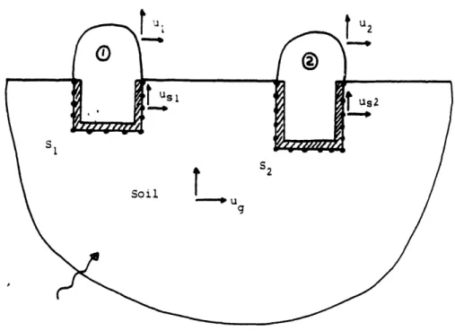
0 (3.14)Assuming the reference point has zero coordinates and using the axis convention shown in figure 3.1, each submatrix of T, corresponding to each node j, is given by
in-plane motion
for u= [ul u u 2 2u2 .l
0 L X U z
under consideration
anti-plane motion Tj = [1]
for u = u ...
0 Y 2
--where the superscript indicates to the structure
(3.16)
Introducing equation 3.14 into equation 3.13 and rearranging some terms, gives
(3.17)
ATu
o= A-U +B.(P-P )
Premultiplying equation 3.17 by TTB- 1results in
29
TTB-1ATu = TTB-1A.U + TTp -TTP
Defining K = TTB-1AT and H = B-IA, equation 3.18 can be written as
T T $
Ku
o- T P .= T(H.U -P )
(3.18)
(3.19)
The term TTP represents the resulting forces and moments on the soil around each structure. Since no external loads are applied to the structures, these resulting forces must equal the inertial loads
TTp =
w
2MuO (3.20)where M stands for the mass matrix of the structures considered and is explicitly given by in-plane case m 0 1 m -z mI 1 x m 1 1 I 1 symm. 0 m 0 -z m 2 2 2
m xm
2 2 2J
2 (3.21) 1 M= 0 2. anti-ane case (3.22)where mi represents the mass of structure i and Ji its mass moment of inertia (Ji
= Joi + (x?+z?)mi; Joi=mass moment of inertia w.r.t. the center of mass); (xi, Zi) are the relative coordinates of the center of mass of structure i with respect to its reference point.
Substitution from equation 3.20 into equation 3.19 leads to
(K-
2M)u
o= TT(H.U-P )
(3.23)
Equation 3.23 can be solved for uo, the rigid motions of each structure,
* *
considering different seismic motions (defined by U and P ). Figure 3.1 shows an example of a model that this formulation can solve. After obtaining the rigid motions of each structure, the resulting displacements at points within the domain can be computed by applying a ficticious load at the location and direction of the desired displacement. Designating by AI the row matrix of the resulting tractions on the boundary nodes of the structures, and BI the row matrix of the resulting displacements, the unknown displacement u is given by (referring to equation 3.11)
u
i -u i
=-
(Tuo-U )+BI(P-P )
(3.24)
where ui represents the displacement due to the incident seismic waves at the point and
direction chosen. Since from equation 3.13, P-P = B A(Tu -U ) = H(Tuo - U ), equation 3.24 can be transformed into
-j
.0CD
CD
z
C
C:)
-L
I_J
D
2
w
O\\ C -J ocr C,, a) .L4 31 cN-J
-0
,_11 C\3.2 Comparison with Numerical Results
3.2.1 Dynamic Resonse of Strip Foundations Embedded in a Stratum
To test the Boundary Element code developed, some comparisons with other numerical results were performed. First, the dynamic compliances of a rigid embedded strip foundation were evaluated and compared with the results obtained by Chang-Liang [9], who used for this purpose the finite element method. Figure 3.2 shows the geometry of the model chosen. The soil was taken as linearly viscoelastic with an internal damping of the hysteretic type, which was incorporated using the Correspondence Principle as explained in Appendix A. The stratum thickness was taken equal'to the total width of the foundation (H/B=2), since with these dimensions the soil-structure interaction effects are important at frequencies close to the lowest natural frequencies of the stratum. The embeddement of the foundation was taken equal to 2/3 its halfwidth (E/B=2/3), the deepest case analyzed by Chang-Liang. A Poisson's ratio of 0.30 and internal damping coefficient =10% were chosen in accordance with the values used in [9]. A massless foundation was analyzed and the results were computed for several values of the dimensionless frequency ao, defined as ao = H/Cs. In the
boundary element analysis, the stratum was divided into 9 equal sublayers and the bottom of the foundation was discretized into 5 constant elements. Some comparisons with a finer discretization, halving each sublayer, were also undertaken for the static case. The dynamic compliances for the in-plane horizontal displacement and rocking were normalized with respect to the corresponding static values and their variations with frequency are displayed in figures 3.3-3.5, where both the real and the (negative of the) imaginary parts are plotted. It can be seen that the results of the two methods agree extremely well in the entire frequency range analyzed, the largest differences being of the order of only a few percent.
RIGID EMBEDDED STRIP FOUNDATION
0 II I C 1: o. f. d 4 A., L, X. X X 0 I "0 'I I I I I I / I III I I I )6 I I
I
C I II
I. 7
C /
~4 -4 r0 a) X O _ W CN e - --TdsT TUOZTIOH >. / II _ I I I I-
0
o
o
o o
- aoueTTdwo OTueUXUa pazTTeZUON
Us W 3 01 l mp Q .-4 -4 0 f-, II I
35
6UTNooH - aoueTTduWoD oTuIeuAa paz t uIuoN
N = 3 oI 0 z Z c I a a Ml ( . .4 .. N I- ct o o o o o
(N II m _ . _ ,-4 CC,-A U) . o ,, e :9 eQ) -l-_ N a) li as c To o ax o n e e i : u u -4 ( W i mU _ I I I I I I I I
t
! 9 I I I I N U, II 0 (o U-) 14 a) '.4 44 o0 (N 1- 09auPTdwoD SBuTdnoD pazTIWuON
u z
a
w Ca
;U x U, (n xl C. r) (1)37 U, U) m.,., :j m -4 Hn/ n uoT4eOT~TlduWv TPlUOZ!JOH 11 m 1w II al 0 II 0
I-II (:¢ N , 3 I1 0 ED S, L IV ·~4 :3 , w Z 3: '4: [-4 u oc a. ': n~ C %0 u U -4 ,.. a C C I C U,c c z E-0 0 U3 . tn W c w a: Ln 0 I D. .
Co so s
dn/-a' UOTqePTJTTdurV 6uTNo W) 3 : Z 41 CA1;I z U E-0c a. 0 'a U Ci. .l) E-, tz O 0 0 t-o m E, u z E-12 x Ln Ch ,.
z
:1. 0 w, N c) 3o t,4 .-rN o-4 0 hao O ln U, 3 u II N0 a) m r14 14 n C m II 3 a N *-4 .-4 -~ = z I I I TB6uV aseqd 39 N CS 11 I m X II N 3: 0 0 I I I 0114 if Ca z ¢ U) 0. I w
z
c
E4 U a 0 a Cu E-x w z C E-Ez u z E-0 wz
0 a. LO w3 x V)*· -
U) X 3: ' X I C o o 0o -,.I o o D0 0 CN 0 °n/Vn uauipaquI o 4;a;~J N II r.,. m N N II N1l M U I ) U) -
-o
:
o X w I I I cJv 3 w 0 z 0 VI 0 z. 0z E-0 0 U0 E-z 0 E-Z F.x 0 E-0cc E-0r Z 0 0 m z 0 a, (n w N 3 II 0) 44 0 0 041
Afterwards, the response of the rigid foundation to vertically incident in-plane shear waves was computed. The displacements of the foundation are referred to the centroid of its bottom, and were normalized with respect to the free-field horizontal displacement at rock level, uR. The results corresponding to the absolute value of the horizontal displacement and rocking are displayed, respectively, in figures 3.6 and 3.7 as a function of the dimensionless frequency a. Figure 3.8 shows the phase angle of the input motions. The ratio of the horizontal displacement of the foundation and the free-field motion at the surface can be seen in figure 3.9. As before, an extremely good agreement between both methods is found in all cases.
These results are very satisfactory if it is noted that while in the Finite Element method the whole stratum depth needs to be discretized (even incorporating consistent boundaries at each side of the foundation) while in the Boundary Element approach only (4+4+5)*2=26 degrees of freedom were needed.
3.2.2 Dynamic Stiffnesses of Surface Strip Foundations Bonded to a Halfspace
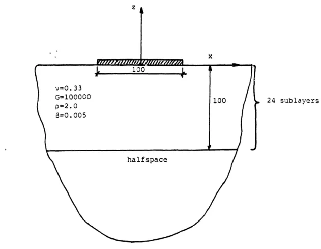
As explained in section 2.2.3, the extension of the Green functions used to the case of a layered halfspace can only be done directly in an approximate way by using a paraaxial approximation for the dynamic stiffnesses of the halfspace. In order to check the accuracy and convergence of such procedure, the dynamic stiffnesses of a rigid strip foundation bonded to the surface of an homogeneous halfspace were computed and compared with accurate numerical solutions given in Gazetas [13], which were computed by a semi-analytical procedure. Figure 3.10 shows the geometry and parameters chosen for this problem. The boundary element results were obtained using constant elements
and modelling the halfspace with a top layer having 100 m (=2B) and divided into 24 sublayers.
The theoretical static stiffness for rocking of a strip footing is
K-
W21
[ + n(-4 (3.26)while the static stiffnesses for in-plane horizontal and vertical displacements of strip footings are zero.
Figure 3.11 shows a comparison of the results using the Boundary Element (B.E.) method with several discretizations (10,20 and 40 nodes) and the value given by equation 3.26 (for a Poisson's ratio of 0.33 and unit shear modulus). The horizontal axis represents a measure of the discretization size and it can be seen that the B.E. results converge almost in a linear way to the exact stiffness. Moreover, if the results corresponding to 20 and 40 nodes are extrapolated linearly, a very accurate estimate of the static rocking stiffness is obtained.
In figures 3.12-3.14, the absolute value of the dynamic stiffnesses for horizontal displacement, rocking and vertical displacement are displayed for a dimensionless frequency ao=1.5 (ao=wB/Cs). Again the B.E. results seem to converge linearly to the more accurate values, except for the rocking mode in which a linear extrapolation gives an error of about 5%.
Overall it can be said that constant elements turn out not to be very accurate for this problem, in particular for rocking, since the extremeties of the foundations have an
43 z L
i
100 L v=0. 33 G=100000 p=2.0 6=0.005 24 sublayers halfspaceFig. 3.10- Strip foundation x
--
m
r
(C--QO'e) sgou;ns OnuvS BZuTpooU · cI C)
W-
coc; to C, 0 ,..II6
11 VI 4)0
I-C) 0 0 0 .4 'o I.,..6a b O 'i:k *j 0 .O0
Co a-E40
Sm .F. ;. 0 0 o o '-i .9-4 0 0 -C 0) 0 0 r- C0 d . M N e 0 eP E D N O NC6
6
6
6
4
4
4
46
., C0 0 II IO C2 i o coD :D c~ .~ c0 m0 'd C2 0 X
co 02 6 6 o - C. cz m c6 C6 a g c2
ci Xj e3 C3 X Q: XX X X
(--90'T.) 9'T=0o
.ZOJ
';TS
JOH
''A-qv
U1 Oc,
P: g
O
0
C3M 0 a PO o o o o o .4 CN a) k4 z 0) .1-1 rZ4 m C C; Oo
(--sO'T ) 'T=0 .zo;',nS 'o o 'A' qv C12 w F-:z ci II 11 2II I, 00 0 9:6 U '-4 0 a 0 .p
I
'4 4I U)i O ctz
a
To 4 C. 0 0 0 0 0o o 0 O b rn 1-1.4 C) w ull Wmi Fa C4 0o 0 00 P 00 10 N -40 a0 0 -0 0m 4 "t6 6
6 66 6
4 44 4
4 41
47 b 4 I m X 2 - k X X i 0 id xi 6 0i vi ' · .4 ,4)iC a o o o ' ) o k
(g-o-'T.) g'T=o' J-.ZoJJ'S '-.teA 'A-'qY
00 Oa) O4 i
CI . 0 av
0 N04 gimportant effect on the response and are not well modelled with constant elements. However, the results are still acceptable, specially if they are corrected for discretization errors. Finally, the paraaxial approximation seems to work well.
3.3 Causality of the Response
When analysing a dynamic problem in the time domain, the response must satisfy the causality relations between any two points. These relations stipulate that the response at an arbitrary point B due to an excitation at point A can only be received (assuming zero initial conditions) after the shortest period of time it takes the fastest wave to travel from A to B, where the travelling path must be contained inside the domain considered. Since the longitudinal waves have the highest speed Cp, and assuming that the only loading is at point A, it can be stated that B-O for t< IB-A I/Cp where
I
B-AI represents the shortest distance between A and B. These causality relations are very important because they follow directly from basic physical considerations, so that any accurate solution must satisfy causality.This problem has recently received much attention as can be seen in the works of Antes and von Estorff [2] and Triantafyllidis et al [43]. In particular, when the domains considered are non-convex, it is important to insure that direct waves travelling in a path passing outside the domain, are not present in the solution. Non-convex domains arise when considering open trenches, tunnels, embedded foundations or even hills as is illustrated in figure 3.15. Antes and von Estorff used a boundary element formulation in the time domain and showed that if the method is applied directly to non-convex domains, the causality condition is not satisfied. However, by dividing the domain into convex subdomains and ensuring compatibility and equilibrium at each new boundary, the results obtained improve substantially. Another possibility to ensure causality of
49
direct wave (physically not possible)
the response in time domain BE. is to check the real shortest travel time between boundary nodes and set automatically the Green's function to zero for lower times and correct them to eliminate the contribution of "direct" waves.
The contribution of "direct" waves in non-convex domains can be associated with the approximations that need to be made in the exact boundary conditions (tractions and displacements). Since the B.E.M. only satisfies these boundary conditions in an integral sense, there are remaining "sources" along the boundary corresponding to the difference between the exact and approximate boundary conditions. These "sources" produce waves which can travel outside the domain and influence directly other points. If finer discretizations of the boundary are used, then the "errors" on the boundary decrease, and consequently, so does the contribution of direct waves. The B.E.M. approximation errors are intrinsic to the method and exist in all boundaries and at all times; however, their effects are particularly relevant in situations where, because of the causality constraint, the response observed should be null. Hence, a measure of the accuracy of the method can be given by verifying if the solution using the boundary element formulation satisfies causality. In particular, when analyzing non-convex domains with stress-free boundaries (open trench or excavation), the boundary element results end to present higher errors since, the stresses being obtained by differentiation of the displacements, they are less accurately represented by the polynomial expansions of the displacements.
Triantafyllidis investigated the causality effects in the boundary element solution to dynamic problems formulated both in the time domain and in the frequency domain. He compared the results obtained in the frequency domain for an harmonic loading in a non-convex domain using a direct approach, with the corresponding solution given by a division of the global domain into convex subdomains, and requiring continuity at their
interfaces. The time lag required by the causality constraint translates into a phase delay for the frequency domain solutions. It was found once more that both solutions have important differences, the latter approach giving more accurate results.
3.3.1 Evaluation of the Resonse to a Ricker Wavelet
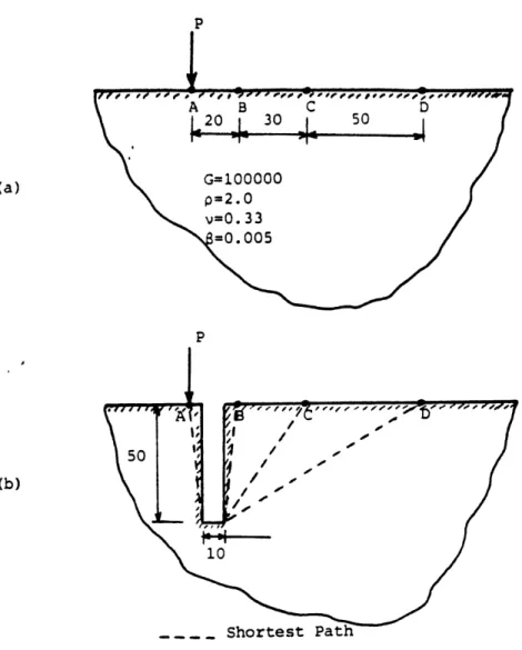
The causality constraint was investigated for solutions obtained by the boundary element formulation described in chapter 2. Since the computations are performed in the frequency domain, results in the time-domain were obtained by Fourier transformation using the fast Fourier transform algorithm. The example chosen consists of an open trench 50 m deep and 10 m wide in a halfspace, and the results were compared to the case in which no trench is present. Figure 3.16 a,b show the geometry of both models and the soil properties. The halfspace was modelled as a stratum with 100 m in depth, divided into 24 sublayers and the paraaxial approximation for the halfspace was added below the stratum. A small internal damping was prescribed (P=0.005) to prevent numerical overflows for the natural modes of the system.
Since the Green's functions used take into account the stress-free condition at the surface, the only boundary discretized consisted of the trench walls and bottom. The boundary element equation 3.13 was modified as follows
A-(U-U ) = B-(P-P )=-B-P
(3.27)
where U and P represent the free-field displacements and tractions of the imaginary boundary of the trench caused by the applied loading; and P=O because the walls and bottom of the trench are stress-free. Hence, the displacements of the trench
p
(a)
(b)
p
Fig. 3.16 - Source and receiver points. (a) No trench; (b) With trench
53
U = U - A-1B .p (3.28)
Knowing the displacements of the trench, displacements at other points in the domain can be computed using a derived form of equation 3.24.
i
= u
i-A (U-U*) -
BIP*
(3.29)
ui representing the displacements at point i in a free-field situation due to the
loading.
The dynamic excitation was idealized as a point load with a time variation of a Ricker wavelet. The Ricker wavelet was chosen, since it decays very rapidly both in time and frequency, thus reducing the number of frequencies to be analyzed. Its equation in time is
f(t) = a(1-2r2) e '
(3.30)
where r = (t-ts)/to; ts is the time at which the maximum occurs, 'a' is the
amplitude, and to corresponds to the dominant period of the wavelet. Figure 3.17 displays a graph of f(t).
The Fourier transform of f(t), F(w), is given by
d ~ ~ D I X : - O _ C- I 0 I I I I I (); To a C) Ee ..
It-0
k ,
u.I I I-Q 4 . CQII Prl 0, S la CL.55 No
0
CQ0
o o CO 4 ~ Q) (3) 50 Cd 51 k4 (1) 0 '14 Q . P4 a CQ U) 1-k Q) C;) ot '.-I 44 0where =wto/2 and w is the angular frequency in rads/sec. A graph of F(w) is shown in figure 3.18 for two different values of to. For this study, to was set to 1/7r,
which corresponds to a dominant frequency of the wavelet near 1 Hz. The time lag ts
was taken equal to to (t=l1/7r) which means that it takes about 0.95 sec for the loading
to attain its maximum.
The solutions in the time domain were obtained multiplying F(w) by the transfer function corresponding to the displacement observed, and Fourier inverting the result (using 8192 points). These transfer functions were computed up to 5 Hz at intervals of 0.10 Hz, and the intermediate values were computed by polynomial interpolation (using Newton's quadrature). The solution in time was obtained at intervals of 0.035 sec.
Figures 3.19-3.21 show a comparison of the results obtained at a point 20 m apart from the loading (point B) for the cases with trench, and without trench. These figures also indicate the shortest time that it would take a shear S or compressional P
wave to reach point B. In figure 3.19, the load and displacement considered are vertical. It can be seen that without the trench, the maximum displacement at B is delayed with respect to the maximum loading by about the time it takes a shear wave to travel from A to B, reflecting the fact that for this direction of loading, the perturbation is transmitted along the surface essencially as shear waves. In the case with trench, the maximum displacement is observed later and corresponds very closely to the extra time it takes the shear waves to contour the trench. Also, at the beginning, the displacement at B is zero for a longer period, reflecting the impossibility for the waves to cross the trench directly. According to these results, it seems that the boundary element formulation adopted satisfies quite accurately the causality constraint of the response.
57 0 0 0 0 0 0 I CA A 0 9 co + 0 '-4 w) A . ~L4 A C Tp` r14
4
-A
0 O0
0
I [LOT). IdoTa Q)0
Pc m1 4-4 ".4 74 O N * a cn 0CI o
II C 11 4.0 ;
0co04 A 0
z
CN + _ 0 I) W) .4 00 q D - j~~~4 0 0 93 To~~T V-4 0~C:9EA ri 130
O
to
0
1
0
0
0
o
0
0
I
0 X c2 cN _ _ I - _ C2 I I I reO'I.j] 'idsa Q) O i co C)0
4-4 C1 II= n
S (d 0 4 0 co CI C.) cbl ) *- 9 4 11 0.) .W 0r igVD
I
A CQ + 0 M , + , 0 kA I
A -4 C o 0 0 [/.o0' tl] 'Idua 59 0) O0 ~4-4.4*tJo
=
.
X
P II Cc0p Co la * 1 MB
co 11 m 0 4i (L) O Cdo
t0
of0
0
0
0
o
o
C _ v C Xin figure 3.20. Again, there is a delay in the time when the maximum response is observed when the trench is present, and this delay is somewhat longer then the difference in travelling times of the fastest shear waves. This may be caused by intermediate reflexions at the walls of the trench. It should be noted that the presence of the trench induces much more important horizontal displacement than would otherwise be observed.
Another interesting observation concerns the comparison of the horizontal displacement at B due to a vertical load at A and the vertical displacement at A due to a horizontal load at B. According to Betti-Maxwell's reciprocity theorem, both should be equal; however, the B.E.M. does not ensure this theorem because of the approximations used at the boundary. Only if the boundary conditions were exactly satisfied could the B.E. solution satisfy the reciprocity relationship. This implies that another test on the accuracy of the B.E. results is to check the reciprocity of the load and displacement in two solutions. Since the domain and reference points considered are symmetric, the vertical displacement at A due to a horizontal load at B is equal to the negative of the vertical displacement at B due to a horizontal load at A. Hence, comparing the results in figure 3.20 with the ones corresponding to a horizontal load at A (in the negative direction) and a vertical displacement at B, a good measure of the accuracy of the solution is obtained. For the case without trench, both results are identical since the Green's functions used satisfy reciprocity; in the case with trench, although some differences were found, they were minimal, less than 1%.
Figure 3.21 corresponds to the case of a horizontal load at A and displacement at B. The displacements at B in the case with trench are very different to the corresponding ones for the halfspace. Instead of the displacements varying in time like the loading function, they are affected by waves reflected at the trench's bottom; this
61
also explains the change in sign of the solution during the initial period. Also, the difference in arrival time of the two peaks observed (one negative and the other positive) approaches the difference in travel time between P and S waves. Therefore, it seems that the motion at B is first caused by P waves and later by S waves.
3.3.2 Comarison with Time-Domain Solution
The results shown in figures 3.19-3.21 were compared with corresponding solutions obtained using a time-domain B.E. formulation presented by Antes and von Estorff [1]. Von Estorff also performed the computations in the time domain for the same cases referred to previously, using either constant or linear elements to model the halfspkce and the trench. In his solution, the halfspace surface had to be discretized as well, since the Green's functions used by him correspond to the full 2-D space. The concentrated loading was idealized as an uniformly distributed load over one element.
Figures 3.22-3.30 show a comparison of the displacements observed at various locations using the two approaches. It can be seen that the solutions agree very well for both vertical and horizontal loads and displacements. The more important differences arise for horizontal displacements due to a vertical load, in particular after the maximum is attained. These comparisons, although corresponding to a very simple problem, served to establish a common ground for the more complex situation with a trench.
The displacements obtained for the case with trench are compared in figures 3.31-3.36. Figures 3.31 and 3.32 correspond to the vertical displacement at B and C respectively, caused by a vertical load. It can be seen that the frequency domain solution seems to satisfy the causality principle more closely, and that in the
cu -3 0 aS
0
0 oa
Oa ,A,.O..te, qdsi63 W Cd '4. ri t 'U IPEIU 0 AG fn r N a 1 0O' o,. k 3 it A
0
* r ,
fij
t
0 a} 0 w_ li ar 0 it, 0 O - q ; to q0
cd P4 'C 4 iC, *C A + A W Ln -a C oN D ) a) -) w a : _ tp 13 2
0w
4) NO t o C') CI - 0 - C CI t o I I I I I [LZaO'Te] 'ds;a 665 C) O P4Co
m 4 (Z2-.) O ..w _ a U) 0 11 9 ._ C *-4PO m .F.ol a aI N -0 N I I I I _ I I I I I -
0
0
rj2
0
4-po nM
X II o4a
Z
-P-1 CM %D 0 o a) k a · 4 : o Ez * Di _o A C( C . it 0 of0
(,&so-T,*] -Tdrs67 w I I I I ! I l.-4 .4 - I I I I [La.O' I] 'IdTa Q Q C
P4
.-=
.
w :.40
-:f ij2
cn0d
.4R .O.) 1 P-co 0 0 so W 4 4) +Gia, o % 4) 0L4 Ur)
CQ 0-0 ^, 0 tl .1-4 44C, ai C2 + co -a CN _ 0 r4
aa
4 cj4 Aq rz 0 0 0 0 0 0 0 0 ,if C:2 C 2 C02 I I [LaO' T] 'Ids(Ta Cd0
p4 cn C12~ -5 P CoOX,
M * 0 C 'S41
It3 X
.. q 2Ir--4 P4 mR69 9e . ccx la To0 0 II X 4) N 4)