Diagnostic experiments in a magnetically driven shock tube.

)CUMENT OFFICE 26-327

.SEARCH LABORATORY OF ELECTRONICS ,SSACHUSETT$ INSTITUTE OF TECHNOLOGY ,MBRIDGE, MASSACHUSETTS 02139, U.S.A.

ii_ i i

4,14'

OApy

DIAGNOSTIC EXPERIMENTS IN A MAGNETICALLY

DRIVEN SHOCK TUBE

JOHN B. HEYWOOD

TECHNICAL REPORT 428

DECEMBER 31, 1964

MASSACHUSETTS INSTITUTE OF TECHNOLOGY

CAMBRIDGE, MASSACHUSETTS

The Research Laboratory of Electronics is an interdepartmental laboratory in which faculty members and graduate students from numerous academic departments conduct research.

The research reported in this document was made possible in part by support extended the Massachusetts Institute of Tech-nology, Research Laboratory of Electronics, by the JOINT SER-VICES ELECTRONICS PROGRAMS (U.S. Army, U. S. Navy, and U.S. Air Force) under Contract No. DA36-039-AMC-03200(E); additional support was received from the National Science Foun-dation (Grant GK-19).

This report will also be issued as Fluid Mechanics Laboratory Publication No. 65-1. Additional support for this work was pro-vided by the Advanced Research Projects Agency (Ballistic Missile Defense Office) and the Fluid Dynamics Branch of the Office of Naval Research under Contract Nonr-1841(93).

Reproduction in whole or in part is permited for any purpose of the United States Government.

SCALES FOR OSCILLOGRAMS

Fig. 8.

VE scale 2 kv/cm; I scale 125 kamp/cm; time scale

2 jisec/cm.

Fig. 18.

Vertical scales in wb/m2; time scale 1 sec/cm.

Fig. 19.

Vertical scales in wb/m2; time scale 1 isec/cm.

Fig. 21.

Vertical scales in wb/m2; time scale 1 sec/cm.

Fig. 24.

Vertical scale 67 volts per cm/cm; time scale

1 sec/cm.

Fig. 26.

Be scale in wb/m

; Er scale in volts per cm/cm; time

scale 1 sec/cm.

Fig. 28. Deflection in 1014 watts/m,

m3, sterad; time scale

d

MASSACHUSETTS INSTITUTE OF TECHNOLOGY

RESEARCH LABORATORY OF ELECTRONICS

Technical Report 428 December 31, 1964

DIAGNOSTIC EXPERIMENTS IN A MAGNETICALLY DRIVEN SHOCK TUBE

John B. Heywood

Submitted to the Department of Mechanical Engineering, M. I. T., September 12, 1964, in partial fulfillment of the requirements for the degree of Doctor of Philosophy.

(Manuscript received November 4, 19 64)

Abstract

This report describes the results obtained from a series of experiments in Hydrogen in a magnetic annular shock tube with an applied axial magnetic field. Measurements of the front speed were made over as wide a range of initial gas pressure, initial drive bank voltage, and axial magnetic field as possible. These results are compared with the pre-dicted speeds obtained from the Kemp and Petschek solutions and the snowplow model, and reasonable agreement is obtained.

Measurements were also made on the front properties with magnetic and electric field probes inside the annulus, and with phototubes. It was found that a substantial frac-tion of the drive current always flows in the front and no shock wave preceding the cur-rent sheet was observed. A detailed picture of the curcur-rent distribution inside the annulus is obtained, and a current loop was found to flow behind the front. It is shown that elec-tric field measurements substantiate this picutre. It is also shown that when the Alfv6n speed ahead of the front is comparable with the front speed, the flow pattern changes significantly.

TABLE OF CONTENTS

I. INTRODUCTION 1

1. 1 General Considerations 1

1. Z2 Magnetic Annular Shock Tube 1

1.3 Experimental Program 2

II. THEORETICAL MODELS FOR THE OPERATION OF A MAST 4

2. 1 Kemp and Petschek Solution 4

2.2 "Snowplow" Model 5

2. 3 Comparison of the Two Models 6

2. 4 Validity of the Assumptions 6

III. EXPERIMENTAL APPARATUS, MEASURING TECHNIQUES, AND

INSTRUMENTATION 8

3. 1 Description of the Experimental Apparatus 8

3. 2 Measuring Techniques and Instrumentation 13

IV. EXPERIMENTAL RESULTS 17

4. 1 Summary 17

4. 2 Measurements on Azimuthal Uniformity 18

4. 3 Measurements of the Front Speed 19

4. 4 Internal Measurements with B₀, Ez, and Er Probes 24

4.5 Absolute Light-Intensity Measurements 39

V. INTERPRETATION OF THE RESULTS 43

5. 1 Summary of Front Properties 43

5. 2 Momentum Balance ₄₃

5. 3 Internal Flow Pattern ₄₅

VI. CONCLUSIONS 47

6. 1 Summary 47

6. 2 Suggestions for Further Work 47

APPENDIX A Diffusion of the Current Sheet into the Shock-Heated Gas 49

APPENDIX B Equation for the Flux Speed 50

APPENDIX C Drive-Bank Performance with the Shock Tube as Load 52

APPENDIX D Calibration of B Probes and Magnetic Search Coils 54

Acknowledgment 56

References 57

I. INTRODUCTION

1.1 GENERAL CONSIDERATIONS

Interest in the dynamics of gases at very high temperatures and velocities has stimulated the development of devices that permit experimental investigation of the properties of such ionized gases or plasmas. One such device is the shock tube. In it the undisturbed gas is accelerated and heated as it passes through a strong shock wave that is driven down the tube. The attraction of this type of device is that the gas com-pressed between the shock wave and the driver interface (called the homogeneous gas sample) has properties that can be accurately calculated from the state of the undis-turbed gas and the conservation laws. A discussion of the conditions attainable in various types of shock tube and some of the limitations of these devices have been

given by Kantrowitz.

The temperatures and velocities attainable in conventional pressure- or combustion-driven shock tubes are limited by the speed of sound in the driver gas. These limits can be raised by adding the energy from a condenser bank to this driver gas (arc-driven

shock tube); but to obtain shock velocities high enough to completely ionize the gas com-pressed behind the shock wave (of order 107 cm/sec for Hydrogen gas) it is necessary to resort to electromagnetic forces to propel the shock down the tube. This type of

driver (called a magnetic driver) involves the interaction between the current obtained from a condenser-bank discharge and the magnetic field that this current creates behind it to drive the current down the tube. If the gas temperature, and thus the electrical conductivity in the current sheet, is high enough (magnetic Reynolds number effect) the current sheet will act as a piston and drive a shock wave in front of it. Shock speeds1 of up to 6 X 107 cm/sec have been obtained with this type of device.

1.2 MAGNETIC ANNULAR SHOCK TUBE

One useful type of device that has been developed has coaxial geometry, in which the driving condenser bank is discharged between two concentric metal cylinders. The radial current sheet that is produced is driven down the annular spacing between the

cylinders by the azimuthal magnetic field which it sets up. Two types of test-gas distri-bution in this annular space have been considered. In one the gas is released at the driving end of the tube from a fast-acting valve. This type of device is usually called a "Plasma Gun" or "Plasma Accelerator."2 '3 _{In the other, the initial test-gas pressure} is uniform; this is called a "Magnetic Annular Shock Tube" (MAST)4 - 8 and it is designed to produce a slug of shock-heated gas whose properties are uniform and can be calcu-lated.

To achieve such a uniform shock-heated gas sample, magnetic containment in the form of steady magnetic bias fields parallel to the walls of the shock tube must be applied, to prevent the hot ionized gas from condensing on the walls. These bias fields

will also interact with the shock front and the driving current sheet, and thus can sub-stantially modify the flow pattern inside the device. Such magnetogasdynamic shock waves have been the subject of extensive theoretical work9 - 1 1 and the results are now well known; however, the relevant experimental results are meager. Patrick1 '4 has extensively studied the case in which initially there is a strong azimuthal and weak axial magnetic field in the annulus. From measurements of the radiated light intensity and the magnetic field inside the annulus, he has shown that under certain conditions a homogeneous gas sample can be obtained, and that the density of the shock-heated gas and the change in field across the shock correspond to the predicted values. Fishman and Petschek6 and Keck5 ' 7 have studied the current-sheet behavior under a wide range of experimental conditions with no initial bias fields. These experiments were carried out in a MAST for which the ratio of the outside to inside radius was large, and thus radial variations become important. The shape of the front, and the current distribution in and behind the front were obtained. The maximum front speeds (-5 cm/[sec) were much less than those obtained by Patrick; and their results show no evidence of a shock wave separated from the current sheet. Heiser8 has done some preliminary work on the effect of an axial bias field and the existence of a switch-on shock. His results, however, show considerable scatter, and a front moving down the tube was observed only in approximately 20 per cent of his experiments. His observed front speeds were approximately 50 per cent of the predicted speed, and the flux speed (see section 3.2a) was approximately 20 per cent of the front speed. Thus it is not clear what flow pattern was set up in his experiment.

1.3 EXPERIMENTAL PROGRAM

The experiments described in this report are intended to provide a detailed picture of the flow pattern inside a MAST when the initial magnetic field is in the axial direction. The experimental program was set up to provide answers to these two questions which had not been considered in detail before. First, do either of the two existing theoretical models considered predict an accurate over-all momentum balance for the device over

a wide range of experimental conditions with an initial axial magnetic field? Second, what is the detailed flow pattern inside the device over a range of axial magnetic fields, and is either of the models considered a reasonable approximation to the observed flow pattern? It was hoped that evidence would be obtained to indicate that the shock sepa-rated from the current sheet, as one of the aims of the project was to develop a device that would produce a gas sample whose properties could be calculated. Of particular interest here was the switch-on shock wave, and it was hoped that the existence of such a shock could be demonstrated. When no evidence of a homogeneous gas sample was obtained, the current-sheet behavior was studied in an attempt to understand why the expected separation did not occur.

This report is arranged as follows. In Section II the two existing theoretical models that are considered are briefly reviewed. In Section III the experimental apparatus,

measuring techniques, and instrumentation are described in detail. Section IV contains a description of the experiments carried out, the results obtained, and an evaluation of the results. Section V includes the interpretation of some of the flow features that were observed, and a discussion of the accuracy of the two theoretical models considered here. Section VI completes the report with conclusions and suggestions for further work.

II. THEORETICAL MODELS FOR THE OPERATION OF A MAST

2.1 KEMP AND PETSCHEK SOLUTION a. Assumptions

Kemp and Petschek9 analyzed an idealized model of the flow pattern in a MAST. They considered the general case for which the initial steady magnetic field has both axial and azimuthal components; only the effect of the axial field is of interest here. A

summary of their results follows.

It is assumed that the current sheet acts as a solid piston (high magnetic Reynolds number) and produces a shock wave in front of and separated from it by a region of

shock-heated gas. These assumptions are made:

(i) variations in the radial direction are negligible, and the problem can be analyzed in Cartesian coordinates with variations in the x (or axial) direction only;

(ii) gas pressure is isotropic;

(iii) gas obeys the perfect gas law with k = 5/3;

(iv) gas has infinite electrical conductivity everywhere; and

(v) drive current is a step function in time and rises instantaneously to a steady value.

The validity of these assumptions for this experiment is considered in section 2.4. Assumption (v) results in the region of shock-heated gas having uniform properties; thus the shock and drive-current phenomena can be treated separately.

b. Effects of Axial Field on the Shock Wave

The effect of a magnetic field normal to the shock wave is well known and has been summarized by Heiser.8 The important points and nomenclature to be used throughout this report will now be discussed.

In shock stationary coordinates, subscript 1 denotes conditions upstream of the shock, and subscript 2 conditions downstream of the shock; u denotes the gas velocity; bx the Alfven speed (Bx/ ); uS the shock speed in laboratory coordinates; and cf

11

the fast magnetoacoustic wave speed. When

us = u1 >Cf > >bx, (1)

s I f 1 2 x2(

shock conditions are not changed by the axial magnetic field Bx perpendicular to the front. [Note that the theoretical models are expressed in Cartesian coordinates with Bx, the axial field, normal to the front. In our experiments the flow parameters are expressed in cylindrical coordinates; thus the axial field will be Bz.] The density ratio across the shock is then given by the usual strong shock limit.

P2 (k2+ (2)

(2)

As B is increased, the condition

u =u 1>Cf >b =u2 (3)

1 2

is reached. The shock jump equations then permit a solution for which a tangential magnetic field exists in region 2 and a current flows in the shock front. This is

appropriately called a "switch-on shock," since the tangential field is "switched-on" by this current. This condition would exist when

s bx k2 -(5)

s 1 k 1'

and the density ratio is now given by

2

P2. (6)

c. Effect of Axial Field on the Expansion Wave

The axial field in cylindrical coordinates introduces a jrBz force in the direction which produces an azimuthal acceleration of the fluid in the current sheet. To reduce this azimuthal acceleration, the current sheet spreads through the gas as a wave. This effect causes a slight increase in the shock speed, and a reduction in the length of the ideal test slug until at a shock speed given by the equality in Eq. 5 the front of the expansion wave is coincident with the shock. For values of u less than this limit, the front of the expansion wave moves back away from the shock, although part of the current is left in the shock front, itself.

Extensive numerical calculations on the shock and expansion wave properties have been done by Kemp and Petschek,9 and when it is appropriate their results will be

com-pared with the experimental data presented in Section IV.

2.2 "SNOWPLOW" MODEL

Another model has been used to describe the performance of this type of device; it is the "snowplow" model. In this model, it is assumed that the gas swept up by the radial driving-current sheet is entrained in the sheet and accelerated to the sheet velocity. Thus a surface mass density can be associated with the sheet at any instant in time, which is equal to the integrated mass density through which the sheet has moved.

The model assumes that the current is confined to a thin sheet, and thus is not applicable for large values of the axial field. It is also assumed that the magnetic Reynolds number in the sheet is high; thus this model represents the limit of the Kemp and Petschek model as the density ratio P2/P1 tends to infinity. The same momentum balance can be

obtained merely by assuming that all of the gas is swept up by the sheet and accelerated to the sheet velocity.

Thus when the axial field is small a momentum balance can be written:

B 2 du

2°o= PlUs + f P1 dz, (7)

where Be is the drive field, and us the front speed. 2.3 COMPARISON OF THE TWO MODELS

When the front speed is constant (it will be shown that this is a good approximation to the observed results), Eq. 7 gives the front or current-sheet speed,

Be

u . - (8)

s 2oP 1

This can be compared with the Kemp and Petschek solution for small axial fields which gives the shock speed

Be 1

- , (9)

s]2oP 1 (1-Pl/P2)1/

and the current sheet speed B0( 1-P 1/P2)1/2

u _{c L2 op 1} . (10)

Notice that the front speed, from Eq. 8, and the shock speed, from Eq. 9, differ only by the factor (1-P 1/P2)1/2. For a strong shock this factor will be between 0.87 and 1.0; the lower limit is obtained when ionization and dissociation are ignored. Thus the pre-dicted value of us does not depend to any marked degree on the choice of model.

2.4 VALIDITY OF THE ASSUMPTIONS

Significant departures from the one-dimensional model, assumption (i), could result 2 from the radial variation of the drive field Be. The ratio of the driving pressure B0 2pLo at the inner and outer radii is given by

2

r°2= 1.9. (11)

r i/

Fishman and Petschek1 2 have considered the effect of annulus ratio (2(ro-ri)/(ro+ri), which is 0.32 for this experiment) in the case for which the initial magnetic field is parallel to the shock front. Their results suggest that for an annulus ratio of 0.32, the one-dimensional model should be satisfactory for Alfv6n Mach numbers less than 5 for an azimuthal bias field. No calculations, however, have been made for an axial bias field, and the flow pattern is significantly different, since the expansion wave moves

towards the shock as the axial field is increased. The validity of a one-dimensional model will be discussed in Section V.

Assumptions (ii) and (iii) have been adequately discussed by Kemp and Petschek, and they conclude that the approximations are reasonable for the equilibrium tempera-tures predicted behind the shock at speeds comparable with those measured in these experiments.

Assumption (iv) has been considered in detail by Kantrowitz, 1 and more elegantly by Falk and Turcotte.1 3 Using these results, we have made calculations of the diffusion of the current sheet into the shock heated gas (see Appendix A). The results show that if the current sheet is preceded by a homogeneous gas sample at the equilibrium shock temperature calculated from the shock speed, then the diffusion of the current sheet for front speeds measured in these experiments should be negligible. But these calculations provide no evidence that this flow pattern will in fact be set up.

Assumption (v) can be satisfied by suitable design of the drive capacitor bank. The bank was set up to provide a square current and voltage pulse, but stray inductance in

the leads and shock tube limited the rise time to 2 Lsec. All measurements were taken after the drive current had attained its steady value, which was between 5 Lsec and 10 1sec after the bank was fired. It was therefore expected that the flow pattern would not change appreciably over a length of order 50 cm.

III. EXPERIMENTAL APPARATUS, MEASURING TECHNIQUES, AND INSTRUMENTATION

3.1 DESCRIPTION OF THE EXPERIMENTAL APPARATUS

A general view of the experimental arrangement is shown in Fig. 1. A schematic cross section of the shock tube is shown in Fig. 2. A photograph of the electrode end of the shock tube is shown in Fig. 3, and an accurate cross-section drawing of the electrodes and current leads in cylinders is shown in Fig. 4. These four figures supple-ment the following text.

a. Shock Tube

The tube itself consists of the annular space between two concentric stainless-steel cylinders sealed at each end with lucite insulators. The outside and inside radii of the annular space are 72 mm and 52 mm, respectively. The tube is mounted inside a 7-inch diameter, 52-inch long, 3 turn per inch solenoid which provides the steady axial mag-netic field. The electrodes consist of two stainless-steel rings of triangular cross section projecting 1/8 inch into the annulus from the two steel cylinders. These rings are mounted 16.7 cm from the driving end of the tube to ensure that breakdown occurs in a region of uniform axial magnetic field. The insulator at the electrode end fills the annulus for a distance of 15 cm to ensure that breakdown occurs at the electrodes; the end of the insulator is capped with a 1/4-inch thick Pyrex glass ring to prevent excess-ive ablation of the lucite by the arc. A set of eight identical search coils, uniformly spaced around the annulus, are mounted inside this insulator to measure the B mag-netic field and ensure that the drive-current distribution into and out of the electrodes

QUARTZ

AXIAL

APERTURE

LENS

FILTER--PHOTOTUBE

Fig. 2. Schematic cross section of the shock tube.

Fig. 3. Detail of electrode end of the shock tube.

9

INLET

OR

E

I) 0

r

is azimuthally uniform. The insulators at the other end of the tube were also covered with Pyrex to reduce ablation from the low melting point lucite that was used to seal the annulus.

Hydrogen, 99.9 per cent pure, was bled continuously through the system to reduce the impurity level to a tolerable value (in all cases it was less than 0.2 per cent by volume). A variable leak valve controlled the flow of gas into a manifold outside the outer cylinder at the electrode end of the tube. The gas flowed into the annulus through twelve 1/32-inch diameter holes uniformly spaced around the circumference, and was pumped out at the other end of the tube through a molecular sieve. The flow rate was adjusted to give the required gas pressure in the system, and this pressure was measured with an Alphatron pressure gauge which was calibrated against a McLeod

gauge at frequent intervals.

Measurements on the front and expansion wave properties were made through 5/16-inch diameter holes cut in the outer steel cylinder. Eighteen of these holes were sealed with quartz windows to permit measurements to be made with photomultipliers of the radiated light intensity, and arrival time of the front at various axial and azimuthal positions. Eight of these windows were arranged along one side of the tube at 15.3-cm intervals, the first being 8.6 cm downstream of the electrodes. The remaining windows were arranged at opposite ends of horizontal and vertical diameters at 39 cm, 54.2 cm, and 69.4 cm downstream of the electrodes so that the azimuthal uniformity of the front could be checked. All windows were mounted flush with the inside wall of the outer cylinder and were cemented in place with epoxy. Four of the holes could be used to insert probes into the annulus at 46.8 cm, 61.8 cm, and 77.2 cm from the electrodes; at 61.8 cm two probe holes and a quartz window were arranged within an arc of 60° in the 0 direction so that three simultaneous measurements could be made at this position. The probes and probe holders were sealed to the tube with "O" rings.

All other seals were made with welded or silver-soldered joints, or with "O" rings. b. Capacitor Banks

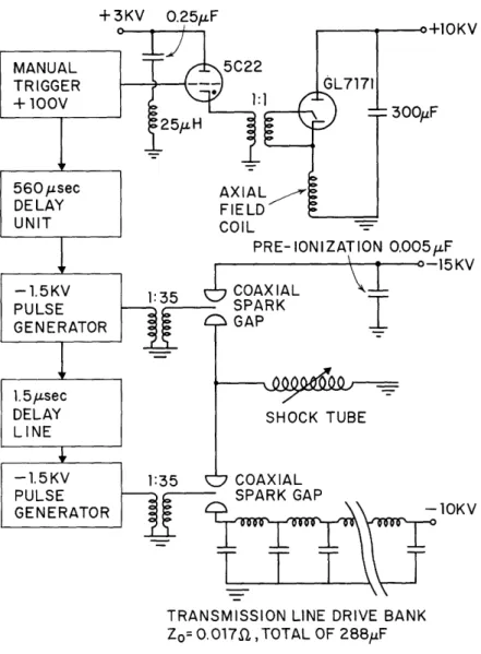
The axial field current, preionization discharge, and drive current were provided by capacitor banks connected to the shock tube through appropriate switching circuits. A schematic circuit diagram is shown in Fig. 5.

(i) Axial field bank

This consisted of five 60-fd, 10-kv capacitors connected in parallel through an ignitron to the axi-al field coil. The quarter-cycle time of the bank-coil combination was found to be 560 Isec, and the maximum field attainable inside the annulus was 0.45 wb/m . A field probe in the axial direction over the center 40 centimeters of the

annulus indicated field variations of less than 3 per cent. The accuracy of the calibra-tion was estimated as 6 per cent.

(ii) Preionization discharge

It was found that a low current (-100 amps) discharge between the electrodes,

+3KV 0.25aF

TRANSMISSION LINE DRIVE BANK Zo= 0.0172, TOTAL OF 288yF

Fig. 5. Schematic circuit diagram and firing sequence.

1.5 ULsec in advance of the main bank triggering, improved the reliability of breakdown, but had no subsequent effect on the flow pattern. Two 0.01-FLfd capacitors at -12 kv were used for this purpose.

(iii) Drive capacitor bank

The drive-current bank was set up with distributed inductance to simulate a transmission line and thus provide a drive-current waveform that approximated a step function. To obtain a characteristic impedance low enough to match 'that of the shock tube, the bank was designed as four parallel transmission lines with eighteen 4-Ifd, 10-kv capacitors in each line. The distributed inductance was provided by parallel copper plates of appropriate dimensions and separation. The impedance of the four lines in parallel was measured to be 0.017 ohm. The high-voltage terminal of the bank was connected to the electrode end of the inner cylinder through a coaxial spark gap, and the ground terminal of the bank to the electrode end of the outer cylinder. A

combination of parallel-plate and low-inductance cable was used to keep the stray inductance to a minimum. Great care was taken to ensure that the azimuthal distri-bution of the drive current leading into and out of the electrodes was uniform. Figure 3 shows the lead in connections used to achieve this end. The bank could be operated at voltages up to 10 kv, and when it was discharged through the shock tube, a current pulse of the order of 300 kamps with a rise time of 2 uLsec and a pulse length of 10 Lsec was produced. A model for calculating the loading placed by the shock tube on the bank is discussed in Appendix C.

In all of our experiments, the shock tube was run with the center electrode and high-voltage terminal of the bank at a negative potential.

3.2 MEASURING TECHNIQUES AND INSTRUMENTATION a. Current and Voltage Measurements

The axial field was measured by monitoring the integrated output of a single loop wound round the outside of the center of the field coil. This maximum measured voltage had previously been calibrated against field measurements made inside the annulus. The error involved in the Bz field measurement was estimated as 6 per cent.

The drive current was monitored by means of a 15-turn, 2-mm diameter coil inserted at the center of the gap between the copper plates leading from the drive bank to the shock tube. The effective area of this search coil was obtained by the procedure outlined in Appendix D, and the coil output voltage was integrated with a calibrated RC circuit whose time constant was 450 pLsec. The field distribution around the lead-in plate was measured with a second calibrated coil in terms of the field on the center line. The integral of this field around the plate gave the correct conversion factor for obtaining the drive current from the measured field at the center line. The error involved in the drive-current measurement was estimated at 6 per cent.

The voltage between the electrodes was measured by means of two identical(to 1 per cent) 10 k2, 200 times attenuators connected to a differential preamplifier.

The voltage induced in a loop that surrounds the annulus in a radial plane (see Fig. 2) was also measured. This was termed the voltage, and from it a flux speed UL7 can be obtained, since it measures the rate of change of flux as the current sheet moves down the annulus. It is shown in Appendix B that when the current I is constant, the voltage $ is given by

= LIuL + ^A, (12)

where L is the inductance per unit length of the tube, A is a term allowing for the dif-fusion of the current through the steel walls, and uL (the flux speed) is the speed with which the current sheet would move axially if it remained confined to a thin layer. An expression for (that part of the voltage that is due to axial movement of the current sheet) with

13

t4= $ - j (13) is given in Appendix B. It is found that the ratio /$ decreases with time, and is approxi-mately 0.8 at the time when most of the experimental measurements were made.

b. Measurements with Photomultipliers

The arrival time of the front at various axial and azimuthal positions could be measured with six photomultiplier systems. Each of these consisted of an RCA 6655A

0 0

phototube with a 4400 A interference filter of half-bandwidth 100 A in front of the tube collector. The tube output was fed directly into a cathode follower. The phototube was connected to the shock tube with either an optical fibre or a simple optical system, and two collimated holes were used to restrict the volume of plasma which could be viewed by the phototube. The rise time of the system was measured to be less than 0.1 Fsec; the transit time of the front past the collimator was approximately 0.02 sec.

One of the phototube systems was calibrated with a tungsten-filament lamp of known horizontal candle power and color temperature, so that absolute measurements of the radiated light intensity could be made.

c. Magnetic and Electric Field Measurements with Probes

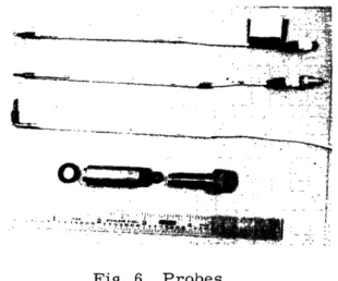
Measurements inside the annulus were also made with magnetic and electric field probes. Considerable time and effort were spent in developing these probes to give reproducible and intelligible signals. Typical probes are shown in Fig. 6, in which the

-aka

n_

·- ,,,,,,·,. ... ,,,

: . .... ... ...L

Fig. 6. Probes.

a 3:1 voltage divider to an RC integrator of (see Fig. 7).

ablated away, the maximum

top probe is a B0 magnetic field probe, the second probe an Er radial electric field probe, and third probe an Ez axial electric field probe. The probe holder is also shown; Fig. 2 illustrates how probes are inserted into and sealed in the shock tube.

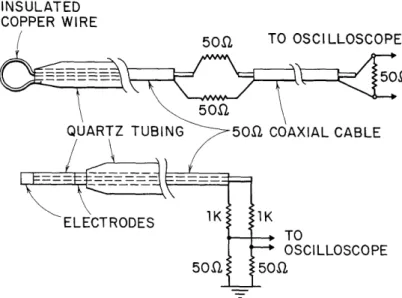
The magnetic field, or B probes, consisted of a single-turn loop, 2 mm in diameter, of #30 Nyclad insulated copper wire mounted outside the end of a quartz

tube and sealed with epoxy. The coil was soldered to a short length of 50-ohm Microdot cable and then connected through time constant 54 ptsec at the oscilloscope The voltage divider was included so that when the insulation on the coil the minimum resistance to ground through the probe was 50 ohms, and voltage at the oscilloscope terminal was less than 600 v. The insulation

INSULATED COPPER WIRE

'SCI LLOSCOPE

(IAL CABLE

;CILLOSCOPE

Fig. 7. Schematic drawing of probe construction.

usually lasted between 5 and 20 runs. The probes were calibrated as described in Appendix D. The probe-to-probe reproducibility was estimated at ±10 per cent (see section 4.4b). When the insulation between the probe and the plasma had broken down, no useful signal was obtained.

Electric-field probes similar to those used by Burkhardt and Loveberg were developed. Figure 7 illustrates, also, the probe construction and circuit. The voltage difference between the two coaxial electrodes was measured by using an identical (0.1 per cent) pair of 1 k2, 20 times attenuators and a differential preamplifier.

Burkhardt and Loveberg have shown under similar conditions that the value of the resistance of the dividers was not important until it was reduced to 5 ohms. The 1-ku value was chosen to give a fast rise time (less than 0.05 sec). The electrode sepa-ration was 0.41 cm for the Er probe, and 0.6 cm for the Ez probe. Only the difference in the floating potential of the probes was measured; this potential may differ from the plasma potential by approximately kT/e. The value of kT/e corresponding to the equi-librium temperature behind the fastest shock observed was 17 volts. This is small

compared with the Er signals (- 200v), but not small when compared with the Ez signals (-40v). Thus the effect of temperature gradients was neglected in the former, and the

Ez probes were used only for qualitative considerations, since substantial errors could be introduced.

d. Firing Sequence

The firing sequence for all experiments and a schematic circuit diagram are shown in Fig. 5. At time T = 0 the axial-field ignitron and the oscilloscope monitoring the Bz field were triggered. At T= 560 ,isec, at the axial field maximum, the preionization circuit was triggered and a pulse sent into a 1.5-ILsec delay line. This pulse then

15

-triggered the main bank spark gap and the oscilloscope monitoring the drive current and electrode voltage at T = 561.5 psec. Breakdown of the drive bank occurred within 0.5 sec. A variable delay was used to trigger oscilloscopes recording phototubes and probe measurements at the appropriate time during the experiment.

The calibration of all oscilloscopes was checked and adjusted when necessary before each set of tests.

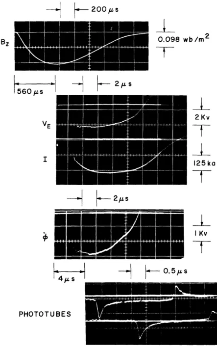
A typical set of axial-field Bz, electrode voltage VE drive current I, voltage, and phototube traces are shown for B = 0.23 wb/m2, initial drive-bank voltage V = 7.5 kv and initial pressure P = 250 microns in Fig. 8.

IV. EXPERIMENTAL RESULTS

4.1 SUMMARY

Our experimental program can be divided into four separate parts.

(i) A preliminary set of experiments was concerned with verifying the azimuthal uniformity of the drive field, and the front position. It was obviously necessary to demonstrate that conditions around the annulus were uniform before detailed measure-ments at any one point could be taken.

(ii) The second set of experiments was aimed at obtaining the operating character-istics of the tube over as wide a range of the parameters P1 initial pressure, Bz axial field, and VO initial drive capacitor bank voltage as possible. Measurements were made of the front velocity us along the length of the tube.

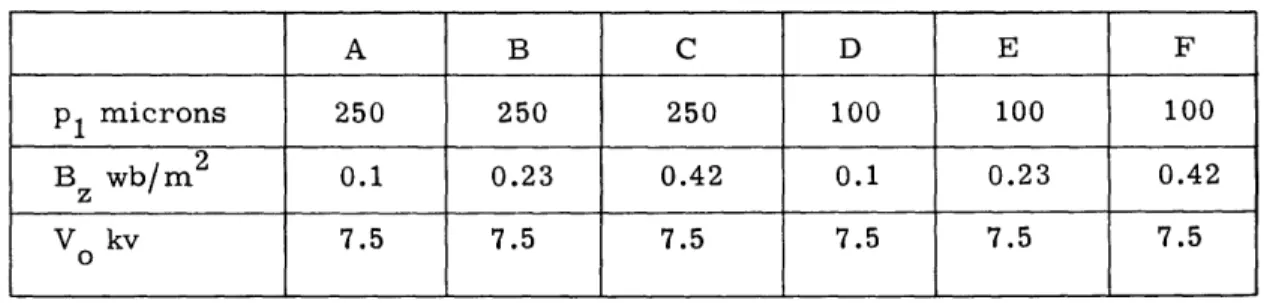
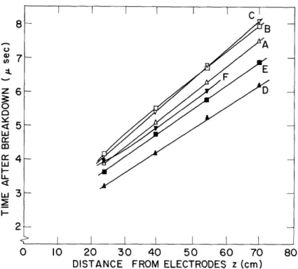
(iii) In the third set of experiments, measurements of Bo, Er, and Ez in the front and expansion wave were made with probes at various axial and radial positions for six selected operating conditions. These six operating conditions were chosen so that the effect of the axial field on the flow pattern at two different pressures could be investi-gated. These conditions will be referred to as A, B, C, D, E, and F in the sequel, and Table I lists the initial pressure P1 and axial magnetic field Bz corresponding to each letter. The initial drive capacitor bank voltage VO was 7.5 kv for each case.

Table I. Experimental conditions.

A B C D E F

p, microns 250 250 250 100 100 100

Bz wb/m2 0.1 0.23 0.42 0.1 0.23 0.42

V kv 7.5 7.5 7.5 7.5 7.5 7.5

O

(iv) In the last set of experiments, absolute measurements of the light intensity radiated by the front and expansion wave were made with a calibrated phototube. It was hoped that these measurements would yield information on the electron density in the gas heated by the front. As we shall see, however, no useful information on the electron density could be obtained.

Before each set of experiments is considered in more detail, some general comments on the reproducibility of the data will be made.

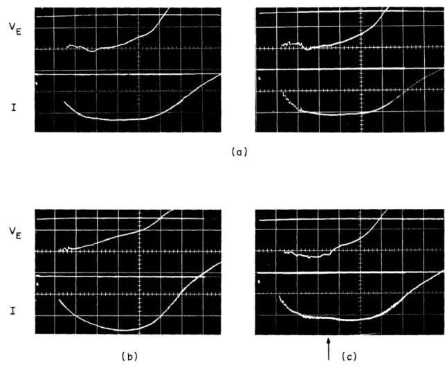
About 80 per cent of the runs made at any given set of conditions satisfactorily reproduced the same flow pattern. Measurements of drive current I and front velocity us were reproducible within 5 per cent. Two drive-current and electrode-voltage traces for similar operating conditions are shown in Fig. 8a. The Bo and Er probe

17

-VE I (a) VE I

(b)

I (c)

Fig. 8. Types of I and VE oscillograms.

measurements were reproducible within 10 per cent; the problem of probe reliability is considered in greater detail in section 4.4a. The Ez measurements were reproducible within 20 per cent; however, the qualitative behavior was unchanged. All of these runs

were characterized by smooth level drive-current and electrode-voltage traces as shown in Fig. 8a.

The remaining 20 per cent of the runs showed drive-current traces in which either the drive current increased steadily throughout the run (Fig. 8b) or a sharp break in the trace occurred when the front arrived at the probe position (Fig. 8c). Data from these two types of runs were discarded. It was also found that at conditions F, the Be and Er measurements showed variations outside the limits quoted above.

4.2 MEASUREMENTS ON AZIMUTHAL' UNIFORMITY

The azimuthal magnetic field between the electrodes was measured with eight identi-cal search coils uniformly spaced around the annulus and built into the lucite insulator (see Fig. 4). The output of each coil was integrated with a calibrated RC integrator (time constants between 320 1Lsec and 420 sec). These signals were compared for

various values of the drive current and axial field, and the shape and magnitude were found to agree within 4 per cent, which is within the estimated error for the measure-ment. It was concluded that the drive-current distribution entering and leaving the electrodes was azimuthally uniform.

Measurements were also made to check the fact that the arrival time of the front at any axial position did not depend on azimuthal position. The maximum time difference measured between arrival times at opposite ends of a horizontal or vertical diameter 39 cm downstream of the electrodes was 0.05 ILsec. This corresponds to a tilt in the shock front of approximately 3 across the mean diameter of the annulus; thus it was considered negligible.

It was therefore assumed in all subsequent measurements that the front and expansion wave properties did not vary significantly with azimuthal position. The simi-larity in shape and magnitude of Bo probe traces from the same axial and radial position, but separated by an angle of 60°, also supported this assumption (see Fig. 16).

4.3 MEASUREMENT OF THE FRONT SPEED a. z-t Diagrams and Flux Speed

Measurements of the front velocity us along the length of the tube were made by measuring the arrival time of the front at positions z = 23.8, 39, 54.2, and 69.4 cm from the electrodes, with four phototubes. A typical oscillogram is shown in Fig. 9. It was found that the front speed was essentially constant from 20 cm to 70 cm downstream of the electrodes; the drive-current pulse was constant (10 per cent) over the corre-sponding time interval. Typical z-t diagrams for conditions A through F are shown in Fig. 10.

The flux speed uL, calculated from Eq. 12 and the appropriate trace, and the front speed us are compared in Fig. 11 for conditions B and D. It was found that the traces changed little between Bz = 0.1 wb/m2 and 0.42 wb/m2 , although the traces at higher Bz were much smoother. The ratio of the flux speed to the front speed will depend on the flow pattern (the Kemp and Petschek model gives uL/us ~ Uc/u s = 0.75; the snowplow model gives uL/us ~ 1). Figure 11 indicates that UL/Us is between these two values, and that the current sheet spreads axially as the front moves down the tube. For times less than 5.5 1Lsec, uL > us. This is because the drive current has not reached its steady value, and thus Eq. 12 is incorrect, since it neglects the dI/dt term. Note also that for T > 8.5 when I declines in value, the calculated uL will be too low for the same reason. Appropriate drive-current traces are included in Fig. 11 to demonstrate when the current is constant.

b. Variation of Front.Speed with Initial Pressure

The variation of the front velocity with initial pressure was then obtained and is shown in Fig. 12 for B = 0.1 wb/m_z 2 and V = 7.5 kv. Front velocities were obtained

19

---,- 200 s 0.098 wb/m 2 -I ' - 1 ' 2,s I R r .. , tv .pv 2Kv

r

-H

0.5 s

Fig. 9. Typical B_z, I, VE' , us oscillograms. Bz

VE

I

4_a4LS

8 n 0L w LL n-4 cr w 3 2 I I I r- 0 10 20 30 40 50 60 70 80

DISTANCE FROM ELECTRODES z (cm)

Fig. 10. z-t diagrams for conditions A through F.

18 16 14 -E J o 8 z ' 6 4 2 0 (L Z 300 _z 200 X n-100 _i: 1+ b r f Y IV

TIME AFTER BREAKDOWN (sec)

Fig. 11. Flux speed and front speed for conditions B and D.

21

I I I I - I I

·

~~~~~~~~~~~~~~~~~~~~~~~~~~~~~~~~~~~~~~~~~~~~~~~~~~~~~~~~

25 20 G) E 10 0) 5 0 I I I l I 30 40 60 80 100 200 400 600 pl (microns)

Fig. 12. Front speed as a function of initial pressure.

by averaging the measured velocity over two adjacent 15.3-cm intervals placed so that the drive current had just reached its steady value at the start of the measurement. The scatter in the observed values of u is approximately 5 per cent. Two theoretical curves are shown; one is obtained from the Kemp and Petschek9

calculations, where their parameter, B/Bo = Bz /(B+B)1/2 is computed from the measured Bz, and Be is calculated at the mean radius (6.2 cm) from the average of the steady values of the drive current measured at a given pressure. The other curve shows the value of u obtained from the snowplow model (Eq. 8) with B calculated as above. Note that the accuracy of the theoretical curve will depend on the accuracy of the drive-current measurement. In addition to errors involved in measuring the voltage output of the search coil-integrator combination (see section 3.2a) a constant error from the cali-bration of the search coil, calicali-bration of the integrator, and integration of the field around the current lead in plate will be present. This constant error was estimated to be within ± 6 per cent.

c. Variation of Front Speed with Initial Drive Bank Voltage

The variation of front velocity with Vo, the initial voltage on the drive bank, is shown in Fig. 13 with P = 250 microns, and Bz = 0.2 wb/m2 . This variation was only attempted at this one pressure, since it was not possible to obtain reliable triggering of the experiment over any appreciable range of drive voltages when the initial pressure was approximately 100 microns. The flux speed uL was obtained from the traces for these runs at the time the current reached its steady value, and the ratio uL/us is also

CHEK SNOWPLOW Bz = O. I wb/m 2 MODEL Vo = 7.5 kv I I I I I I I I I I I I l

I I I I I 16 2 4 6 V o (kv) 8 10

Fig. 13. Front speed and flux speed as a function of initial drive bank voltage.

1.0

0.5--_.J

included in Fig. 13. Theoretical curves for the Kemp and Petschek and snowplow models are shown; the experimental points lie between the two curves.

d. Variation of Front Speed with Axial Magnetic Field

The effect of the axial field was considered at two initial pressures (250 and 100 microns) and V = 7.5 kv. The measured front speeds, and Kemp and Petschek and snowplow model theoretical curves are shown in Figs. 14 and 15. Note that the

14 12 10 8 6 2 2 0 0.1 0.2 0.3 Bz (Wb/m2) 0.4 0.5

Fig. 14. Front speed as a function of axial magnetic field with P₁ = 250 microns. 23 14 12 a) E 8 U 6 4 2 KEMP PETSCI PLOW "'L pi = 250 microns Bz= 0.2 wb/m 2 o us - A UL/Us I I I I u E u m I I I I I

KEMP AND PETSCHEK MODEL

0S ° 0- NOWPLW 0----SNOWPLOW MODEL p1 = 250 microns VO: 7.5 kv I I I I I I I I I I N___ _

20

as 15

I

E

5

Fig. 15. Front speed as a function of axial magnetic field with P = 100 microns.

0 0.1 0.2 0.3 0.4 0.5

Bz (Wb/m 2

)

measured front speeds decrease slightly as B is increased; a trend that was also observed by Heiser. The drive current (which is obviously proportional to the value of us predicted by the snowplow model) remains almost constant over the whole range of B considered in both cases.

z

4.4 INTERNAL MEASUREMENTS WITH B, Ez, and Er PROBES

a. Summary

To obtain more detailed information about the flow pattern inside the annulus, sets of probe measurements were made with the B, Ez, and Er probes described in

section 3.2c. These measurements were designed to answer the following questions. (i) Does all of the drive current move down the tube with the front, or is part of it left at the insulator face to cause ablation of material from the insulator (see Keck7)? Obviously the momentum balance will be incorrect if appreciable ablation occurs.

(ii) Does the shock front (as identified by the phototube output) separate from the current sheet (Be trace rise) for values of axial field when a homogeneous gas sample should exist? If no such separation is observed, then the Kemp and Petschek model will not be applicable.

(iii) Can any change in the flow pattern be observed at the point where the switch-on shock could exist?

(iv) What is the shape of the front? Previous experiments by Keck5 and by Burkhardt and Loveberg3 have shown that the front is approximately planar when the center electrode is negative, and bullet-shaped when the center electrode is positive.

(v) What is the variation of B with radius?

(vi) Can an axial electric field caused by charge separation be observed in the front? This would provide a way of identifying the shock front by using the theoretical work of Jaffrin.14

24

I I I IMODEL

KEMP AND PETSCHEK MODEL

SNOWPLOW MODEL _8 ? I o 0 88 pl = 100 microns Vo= 7.5 kv I I I I I

(vii) What information can be obtained about the gas velocity from radial electric field measurements?

The results will be discussed in the order in which they provide answers to these questions. Some remarks on the validity of the probe measurements will be given first.

It is important to show that probes inserted into the annulus do not affect the flow pattern in any significant way. Obviously, the probe will cause changes in the velocity, temperature, and pressure in the region close to and downstream of the probe. But if it can be shown that the current distribution remains essentially unchanged, then such features as the front speed, and the Be and E distribution should not be affected. When the local axial velocity of the gas is important, as in the Er measurements where a large part of the signal is the inductive uzBo voltage, then the probe output must be interpreted with more caution.

While it could not be demonstrated conclusively that the over-all flow pattern was not changed in any significant way, the following evidence suggests that this assumption is justified.

We found that some of the drive-current and electrode-voltage traces showed abrupt changes in slope (see Fig. 8c) when the front reached the probe position. This some-times occurred when the insulation of the probes broke down. These data were dis-carded; it was concluded that the probe had appreciably changed the flow pattern, and thus the load on the drive capacitor bank. Second, it was found that when the drive-current and electrode-voltage traces were smooth (80 per cent of the runs) neither the number nor the position of probes inserted into the annulus appreciably affected the value of the front velocity or the signals recorded at each probe. Against this, however, must be set the fact that on dismantling the tube, black marks downstream of the probe positions were observed on the steel cylinders, thereby indicating that a wake had formed behind the probe and that material (from the epoxy seal, for example) was being transferred from the probe to the flow.

In the experiments on the axial and radial variation of Be that will be reported next, measurements at any given Pl, Bz, Vo, z, and r were made with at least two different probes. This was done to ensure that any individual probe peculiarities would be immediately apparent.

b. B Measurements as a Function of Axial Position

Figure 16 demonstrates the reproducibility of B8 probe measurements. Figure 16a shows the probe-to-probe reproducibility for the same run at the same axial and radial position; Fig. 16b shows the shot-to-shot reproducibility of the same probe for three runs. For conditions F, however, the reproducibility was greatly inferior.

The azimuthal magnetic field is given by

B _{where V is the voltage read from the oscillogram (as described in} = 3RC VI _A (14) where V is the voltage read from the oscillogram (as described in Appendix D). The

l1 s

Be MAX.

0.8 wb/m2 Be MAX. 0. 81 wb/m 2

Fig. 16. Oscillograms showing

(a) reproducibility of Bo

probes.

0.33 wb/m2

-T

(b)

error in calibrating and positioning the probe, and in calibrating the integrator, is esti-mated as 8 per cent. The important features of the signal are the sharp rise in B as the front passes the probe (the rise time is approximately 0.1 psec, corresponding to a distance of 1.5 cm), and then a more gradual rise to a maximum B from 1 to 2 sec later. It will be seen, however, that under some conditions the front and the rise to maximum Bo cannot be separated.

To investigate how much of the drive current moves down the tube with the front, measurements of B were taken at distances z = 46.8, 61.8, and 77.2 cm from the electrodes at the mean radius (6.2 cm) for conditions A through F. The change in B0 across the clearly defined front and the maximum value of Be were measured from each oscillogram. These measurements were nondimensionalized with the value of the field (BI) calculated at the appropriate radius, from the drive-current value at the time the Be measurement was made. The ratio

Be 2rrBe(t)

B.

(15)

I LoI(t)

I I I I I I m I I I 40 50 60 70 80 A z(cm) I I I I 40 50 60 70 80 B z(cm) 0 A I I I I I v40 50 60 C 70 80 z(cm) 1.0 Be BI 0.5 0 1.0 BI 0.5 0 1.0 Be BI 0.5 0 I I 40 50 60 70 80 D z(cm) fi fI i A 40 50 60 70 80 E z (cm) I I I I I 8 A A A 40 50 60 70 80 F z(cm)

A MEASURED AFTER FRONT o MEASURED AT MAXIMUM

o MAXIMUM AT FRONT

Fig. 17. B/B I as a function of axial position for conditions A through F.

is plotted against z in Fig. 17 for conditions A through F. The ratio of maximum Be to BI should be unity if all of the drive current passes the probe and measurements are made during the time the drive current is constant.

The interpretation of the results is complicated by evidence presented in section 4.4d that current loops flow in the gas behind the front. The measurements of maximum field indicate, however, that with the exception of condition F, 90-100 per cent of the total drive current flows past the probe at the mean radius at each axial position. In Fig. 18 two sets of Be traces are shown to illustrate that the shape of the profile (substantially different for each case) changes little along the length of the tube, although the position of the Be maximum moves away from the front with increasing time. This agrees in a qualitative way with the plots of flux speed uL shown in Fig. 11 where uL decreased with time and uS was constant.

27 1.0 B_e BI 0.5 1.0 Be B1 0.5 0 1.0 Be B 0.5 0

z =46.8cm 0.33

T

i

T

t1~

Fig. 18. Oscillograms of B_e profiles at z = 46.8, 61.8, and 77.2 cm, and the mean radius for conditions B and D.

c. Comparison of Light Intensity Front with Be Front

In this set of experiments, simultaneous measurements were made at z = 61.8 cm with a B. probe at the mean radius, and with a phototube arranged so that the collimated holes of the phototube collecting system and the probe were separated by an angle of 300 in the azimuthal direction. The two signals were displayed on the same oscilloscope, and the arrival times of the two clearly defined fronts were compared over the range of conditions A through F.

With the exception of condition F (where a clearly defined light-intensity front was not always observed), the light-intensity front was always slightly behind (-0.05 sec) the B front. This time difference was not considered significant, since it was of the order of the difference in transit times for the signals through the two measuring circuits. Thus within times of less than 0.05 pFsec, the two fronts were coincident; therefore, one must conclude that the drive current flows at the shock front and no homogeneous gas sample collects between the shock and the current front. Precise agreement with the Kemp and Petschek model would not therefore be expected.

28

i

d. B Measurements as a Function of Radius The B8 probes were then used to measure: (i) the tilt of the front,

(ii) the variation of Be with radius over the range of conditions A through F.

The tilt of the front was obtained by measuring the arrival time of the front at two B( probes, one close to the inside wall, the other close to the outside wall at z= 61.8 cm. The probes were separated in the direction by an angle of 60°; therefore, the azimuthal

symmetry of the front as it approached the probe positions was important. This was checked with phototubes at two windows 90° apart, 7.6 cm upstream of the probe positions. After correcting the arrival times for any slight difference in arrival time from the phototube traces, the maximum differences in arrival times at the probes corresponded to a tilt across the 2-cm annular space of 25° from the normal to the shock-tube axis. These data are in agreement with the measurements3'5 mentioned in section 4.4a (the center electrode was run at a negative potential, and it was found that the front was approximately perpendicular to the tube axis).

Measurements of Be were then made at r = 5.5 or 5.6 cm and r = 7 cm; at z 61.8 cm; for conditions A through F to obtain the radial variation of Be. Typical oscillograms for conditions A through F for r = 5.5 or 5.6 cm and r = 7 cm are shown in Fig. 19. (Bo profiles at the mean radius (6.2 cm) and this axial position are shown in Fig. 26.)

As before, the value of B after the clearly defined front and the maximum B8 were measured and nondimensionalized with B calculated at the appropriate radius from the measured drive current. Plots of Be/BI as a function of radius r are shown in Fig. 20. The values of B(/B I from the previous experiments at z = 61.8 and the mean radius are also included.

It is immediately apparent that the simple model of the drive current moving down the tube as a confined sheet is inadequate for all of the conditions considered. Probes close to the inside wall record values of B8 -50 per cent greater than the field resulting from the drive current alone; although it is found that with the exception of conditions F the current in the sharply defined front corresponds to the field caused by the drive current within ±15 per cent. Close to the outside wall, the maximum field measured was always less than the calculated BI, and the rise time of the front increased sub-stantially. It was felt that the 5/16-inch diameter hole in the outer steel cylinder through which the probe and probe holder were inserted would disturb the distribution of current flowing in the wall. Thus the field measured close to this probe hole may not be the same as the field existing close to the outside wall away from any probe holes.

To investigate the current distribution both in and behind the front in greater detail, a radial traverse was made with a single B probe at conditions B and z = 61.8 cm. This particular set of operating conditions was chosen because the flow pattern appeared

29

r (cm)

Fig. 19. Oscillograms of B0 profiles at z = 61.8 cm, r = 5.5 or 5.6 cm, and r = 7.0 cm, for conditions A through F. 0.33

T

T

T

T

i

T

T

-T1

T

T

T

T

T

I

D A 6 r (cm) 7

-

8

a

8

9

8

Fig. 20. Be/BI as a function of radius at z = 61.8 cm for conditions A through F.

31 1.5 1.0 B8 BI 0.5 0 -aA

f

8

r = 7.0 cm 0.39

t

T

T

r =5.5 cm

Fig. 21. Four oscillograms from Be radial traverse at z = 61.8 cm, and condition B.

to be particularly reproducible. Four of the oscillograms are shown in Fig. 21. Note that the shape of the profile changes substantially with radius. The values of Be/BI after the front, and the maximum values were obtained and are shown in Fig. 22 as a function of radius. The rapid fall off in B0/B I at radii close to the outside wall supports the supposition that the decrease is due to the probe hole in the wall. If this were not the case and the measured field does correspond to that existing close to the wall away from any probe holes, then axial currents of the order of the drive current must flow in the 0.5 cm close to the wall.

With this explanation in mind, Fig. 22 shows that the current flowing in the front over most of the annulus is 10-20 per cent greater than the drive current. While this

I

1.0

cn

0.5

Fig. 22. Plot of B 0/B I as a function of radius for radial traverse at z = 61.8 cm, and condition B.

V 5 6 7

r (cm)

difference is only just outside the experimental error involved in the measurement, it does agree with the values obtained from two different probes (see Fig. 20b).

A current map showing the approximate current distribution in the front and the expansion wave behind it, can be obtained from the four traces shown in Fig. 21. The current density at any point in the annulus is given by

1 aBe Jr = ir

~F

since a/a80 = 0, Bz is constant and it is assumed that any Br that is due to currents in the 0 direction can be neglected. If it is further assumed that the gas velocity behind the front is approximately constant (see section 4.4f), and the current distribution does not change significantly with z (see section 4.4b), then Eq. 16 can be replaced by the approximate expressions 1 AB0 Jr 4o uAt (17) 1 A(rB0) Jz 0r Ar

These current densities can be evaluated from the oscillograms at a series of points in the annulus. Then, by integrating between pairs of points, the actual current distribution can be obtained. It is shown in Fig. 23a, where u was assumed to be 10 cm/psec, and the front was arbitrarily taken to be perpendicular to the tube axis. Any variation in u

33 Be MAXIMUM o 6 7 A o

/aL

I_-o 4 o 0 C CU z u o L Z ' v N o Ac en e0 -4 \ 2 0 - LiL 34 E c" .L 2 1r Li

:I

will merely alter the z-length scale. Since no measurements were made within 3 mm of the walls, r and jz were not computed in these regions, and the constant-current lines (shown dashed) are only estimated. The map shows that a closed-current loop of

105 amps flows in the gas behind the front spread out over a distance of -18 cm axially. Part of this loop flows at the front; thus B after the front is 15 per cent greater than BI . The center of the loop lies between the mean and inside radii, where B maximum is 50 per cent greater than BI . The loop is shaped so that B near the outside radius falls off more rapidly than Be near the inside radius.

Since the field changes with radius and time were often small, this map is only an approximate solution to Eq. 16. Additional evidence to support this flow pattern is therefore desirable. Accordingly, axial electric field measurements were made with the Ez probe described in section 3.2c in the regions where the current flow was pre-dominantly axial. A radial traverse was made at conditions B and z = 61.8 cm, and four oscillograms are shown in Fig. 24. A deflection upwards from the zero line corresponds to an electric field pointing toward the shock front. The sharp rise in the E signal was found to correspond to the arrival of the sheet at the B probe. The important characteristics of the traces are listed below.

(i) An initial sharp spike occuring in the front. It was concluded that this is caused by charge separation, and its mag-nitude will be considered.

(ii) A region of Ez directed toward the shock of approximate magnitude 60 v/cm almost independently of radius and lasting 0.8 Utsec (-8 cm).

(iii) Close to the inside wall an abrupt change in the direction of E at 0.8 sec from the front; close to the outer wall, a gradual reduction in Ez but no change in direction.

E __rete toar From tnese traces, regions o positivethe f_._ __ -____rot an negtiv Ez (directed toward the front) and negative Ez (away from the front) can be obtained; these are shown in Fig. 23b. A compari-son with the current map shows in a quali-tative way that axial electric fields do

exist to drive the current lnnn. lthnih

Fig. 24. Four oscillograms from E the line of zero E falls above the line radial traverse at z= 61.8 cm, joining points where jz = 0. Exact

agree-and condition B. ment should not be expected, however, as

35 r = 7.0 cm

r = 6.6cm

r = 6.3 cm