Distance makes the difference in thermography for ecological studies

HAL Id: hal-01252069

https://hal.archives-ouvertes.fr/hal-01252069

HAL is a multi-disciplinary open access archive for the deposit and dissemination of sci-entific research documents, whether they are pub-lished or not. The documents may come from teaching and research institutions in France or abroad, or from public or private research centers.

L’archive ouverte pluridisciplinaire HAL, est destinée au dépôt et à la diffusion de documents scientifiques de niveau recherche, publiés ou non, émanant des établissements d’enseignement et de recherche français ou étrangers, des laboratoires publics ou privés.

Distance makes the difference in thermography for

ecological studies

E. Faye, O. Dangles, S. Pincebourde

To cite this version:

E. Faye, O. Dangles, S. Pincebourde. Distance makes the difference in thermography for ecological studies. Journal of Thermal Biology, Elsevier, 2016, 56, pp.1-9. �10.1016/j.jtherbio.2015.11.011�. �hal-01252069�

Distance makes the difference in thermography for ecological studies

E. FAYEa,b,c, O. DANGLESa, S. PINCEBOURDEd

a

UMR EGCE, IRD-247 CNRS-UP Sud-9191, 91198 Gif-sur-Yvette cedex, France.

b

Sorbonne Universités, UPMC Univ Paris 06, IFD, 4 Place Jussieu, 75252 Paris cedex 05,

France.

c

Pontifica Universidad Católica del Ecuador, Facultad de Ciencias Exactas y Naturales,

Quito, Ecuador.

d

Institut de Recherche sur la Biologie de l’Insecte, UMR 7261, CNRS – Université

François-Rabelais de Tours, 37200 Tours, France.

Corresponding authors: Emile Faye - ehfaye@gmail.com; Sylvain Pincebourde -

2

Abstract

Surface temperature drives many ecological processes and infrared thermography is widely

used by ecologists to measure the thermal heterogeneity of different species' habitats.

However, the potential bias in temperature readings caused by distance between the surface to

be measured and the camera is still poorly acknowledged. We examined the effect of distance

from 0.3 to 80 m on a variety of thermal metrics (mean temperature, standard deviation, patch

richness and aggregation) under various weather conditions and for different structural

complexity of the studied surface types (various surfaces with vegetation). We found that

distance is a key modifier of the temperature measured by a thermal infrared camera. A

non-linear relationship between distance and mean temperature, standard deviation and patch

richness led to a rapid under-estimation of the thermal metrics within the first 20 m and then

only a slight decrease between 20 to 80 m from the object. Solar radiation also enhanced the

bias with increasing distance. Therefore, surface temperatures were under-estimated as

distance increased and thermal mosaics were homogenised at long distances with a much

stronger bias in the warmer than the colder parts of the distributions. The under-estimation of

thermal metrics due to distance was explained by atmospheric composition and the pixel size

effect. The structural complexity of the surface had little effect on the surface temperature

bias. Finally, we provide general guidelines for ecologists to minimize inaccuracies caused by

distance from the studied surface in thermography.

3

1. Introduction

Surface temperature drives many physical, chemical, biological and ecological processes and

is among the most influent factors for life across all biomes including marine, terrestrial and

freshwater ecosystems (Oke 1987; Kingsolver 2009). Several methodologies have been

developed to measure surface temperature. Among them, infrared thermography is the only

non-invasive method that provides a continuous capture of surface temperature, and major

developments over the past decade significantly improved our understanding of

temperature-related patterns in ecological sciences (Quattrochi and Luvall 1999; Cilulko et al. 2013;

Lathlean and Seuront 2014). Originally, infrared thermography was developed mainly for

industrial, medical and military applications (Vollmer and Möllmann 2010). It was first used

for ecological research in the late sixties (e.g. studies on seal thermoregulation, Ørtisland

1968, and on white-tailed deer detection, Croon et al. 1968). Over the last four decades,

infrared thermography has been increasingly used in various fields of biology including

thermal physiology (Hill et al. 1980; Pincebourde et al. 2012; Woods 2013; McCafferty et al.

2013), marine ecology (Lathlean and Seuront 2014), plant sciences (Jones 2002; 2013;

Pincebourde and Woods 2012; Caillon et al. 2014), agronomy (Jackson et al. 1981; Inagaki et

al. 2008; Meron et al. 2010; Bellvert et al. 2013), and landscape ecology (Scherrer and

Koerner 2010; Tonolla et al. 2010; Faye et al. 2015).

Infrared thermography is an imaging method that records infrared waves emitted by an

object in the electromagnetic spectrum after the visible range of light – from 7.5 to 14 µm –as

a result of molecular motion (Vollmer and Möllmann 2010). Radiation readings are then

converted into surface temperature by the Thermal Infra-Red (TIR) camera taking into

account ambient conditions and object’s emissivity. TIR images allow the study of surface

temperature patterns over a broad range of spatial scales from sea and land surface satellite

4

2015) and organism scales (Tattersall and Cadena 2010; Pincebourde et al. 2013). Recent

advances in thermal imaging technology – increasingly lightweight and hand-held – and a

reduction in the cost of thermal cameras have facilitated its uses and opened new areas of

investigation in ecological sciences (Lathlean and Seuront 2014; Faye et al. 2015).

However, despite its increasing use, relatively few studies have addressed the potential

pitfalls and limits of thermal imaging (Clark 1976; Quattrochi and Luvall 1999; Minkina and

Dudzik 2009; Cilulko et al. 2013; Lathlean and Seuront 2014). Weather conditions (e.g. solar

radiation and rainfall) are known to affect TIR outputs leading to misinterpretation of

organism body temperatures. Also, emissivity of an object – i.e. the ability of an object to

emit thermal radiation – and viewing angle between the camera and the object can affect

surface temperature measurements (Clark 1976). Last, the distance between the object and the

TIR camera (i.e. shooting distance) is among the main factors supposed to impact temperature

values in TIR images (Nienaber et al. 2010; Cilulko et al. 2013). Like any image, TIR images

are composed of pixels, and the portion of object surface area included in a single pixel

directly depends on shooting distance – with larger area included in each pixel as shooting

distance increases. Then, when the surface is thermally heterogeneous, neighbouring surface

patches of different temperature merge together with increasing distance. To our knowledge,

however, the net effect of increasing shooting distance on temperature readings by TIR

camera has never been quantified. At best, TIR images are acquired at equal distances from

the study organism allowing accurate estimates of relative temperature differences between

patches (Inagaki et al. 2008; Tonolla et al. 2012; Caillon et al. 2014).

Here, we examined the effect of shooting distance (in the range of 0.3 to 80 m) on TIR

thermal metrics that are commonly used to quantify the spatial heterogeneity of object

temperatures (e.g. mean temperature, standard deviation, patch richness and aggregation). The

5

shooting distance, 2) to assess the effect of weather conditions (solar radiation) on this

relationship, and 3) to test whether the structural complexity of the studied surface affected

this relationship. We first shot the same object surface (a thermal test card corresponding to a

regular mosaic of black and white patches) under various global solar radiation levels with

two similar TIR cameras placed at different distances. We then shot three object surfaces with

different structure under identical global solar radiation with the two TIR cameras placed at

various distances. Object surfaces consisted in a thermal test card under constant

environmental conditions in the laboratory, a green wall covered by a deciduous woody vine

scene, and an oak-beech forest edge offering a more complex scene. Additionally, we

performed a TIR close-up shooting (0.3 m) of the plant leaves to assess how actual leaf

temperatures shaped the surface temperature distribution at each shooting distance and to

compare the micro-scale thermal heterogeneity of leaves to overall surface heterogeneity.

Generally, we expected that the distance between the thermal camera and the studied object

would lead to errors in the surface temperature because of the pixel size effect. We also

expected this bias to be more pronounced when the surface is heated by solar radiation.

Finally, under similar abiotic conditions, structurally complex surfaces are supposed to

deliver more thermal heterogeneity than simpler ones and we hypothesized that the

temperature measurements of these complex surfaces would be more influenced by shooting

6

2. Materials and Methods

2.1. The thermal infrared cameras

TIR images were acquired using two similar TIR cameras recording long-wave infrared

radiation emitted by objects in the spectral range from 7.5 to 14 µm. They were equipped with

uncooled micro-bolometer sensors and converted infrared radiation readings into

temperatures within the -20 to 120°C calibration range. TIR images were processed assuming

an emissivity of 1 for every surface because our interest was to quantify the discrepancies in

spatial thermal heterogeneity between TIR images of the same surface taken at different

distances – i.e. comparing relative values instead of measuring actual temperature values

(Clark 1976; Rubio et al., 1997). Therefore, surface temperature refers to the brightness

surface temperature in this work (Norman 1995). The surfaces we studied were almost

entirely composed by vegetation, and mostly by leaf tissues. Emissivity of temperate tree

leaves ranges between 0.95 and 0.98 (Gates 1980). A change in emissivity within this small

range causes very small change in temperature readings. We are therefore confident that

potential emissivity variations within the scenes did not cause the bias we observed. The first

TIR camera (called fixed TIR camera, see below) was equipped with a 320 × 240 pixels

micro-bolometer focal plane array (B335, FLIR Systems, Wilsonville, OR, USA). The second

TIR camera (called mobile TIR camera, see below) was equipped with a 640 × 480 pixels

micro-bolometer focal plane array (HR research 680, VarioCAMs, InfaTec GmbH, Dresden,

Germany). For practical reasons, we did not use two identical TIR cameras. Therefore, we

verified that the slight technical differences between the two cameras do not cause bias in

surface temperature measurements (Online Resource 1). We shot studied surfaces

simultaneously with both TIR cameras placed at each shooting distance from 2 to 80 meters

(see Online Resource 1 and below for details). We found no significant differences between

7

shooting distance did not significantly affect the small discrepancies between the two TIR

cameras (Mann-Whitney-Wilcoxon Test, P = 21.92 and 13.48 for mean and standard

deviation respectively). Thus, the two TIR cameras yielded similar temperature readings.

2.2. Experimental design

2.2.1. Thermal test card in different environments

We studied a 1 m2 thermal test card, made of 400 black and 400 white tiles of 2.5 cm2 each,

which delivered a well-characterized geometry and dimensions resulting in a predictable

thermal pattern, with the black tiles reaching higher surface temperatures than the white ones

when hit by radiation (Fig. 1). We placed the thermal test card vertically in three different

environments that differed in term of abiotic parameters (exposure, temperature and global

solar radiation). The first environment – the laboratory environment – was a 50 m long

corridor without window in our laboratory (Institut de Recherche sur la Biologie de l’Insecte,

Tours, France) wherein air temperature and humidity were maintained constant by an

air-cooling system, thereby resulting in a homogeneous environment along the hall (21.7°C and

63% of humidity; Online Resource 2). Global radiation was generated using two 250 W metal

halide bulbs (Sylvania Britelux HSI-T SX clear) positioned on the ground one meter in front

of, and oriented toward, the thermal test card (A.1 and A.2 in Fig. 1). These lamps emitted

both in the visible (37% of total radiation) and in the near infrared range (63% of total

radiation) with a spectrum similar to solar radiation.

The second and third environments were outdoor, at the castle named Château de

Saché in the Loire Valley, France (49°14’45’’N, 0°32’41’’E, at a mean elevation of 77 m

a.s.l.). In July 2013, when the study took place, mean daily temperature reached 20°C (27.7

and 13.9 °C for mean maximum and minimum respectively) and photoperiod lasted almost 10

8

highest vegetation density in canopies at that time (Koerner and Basler 2010). We first placed

the thermal test card in front of a South-exposed green wall of the castle – the green wall

environment – facing a flat area free of any obstacles (B.1 and B.2 in Fig. 1). Then, we

positioned the thermal test card in front of a West-exposed wood edge in the court of the

castle – the wood edge environment – facing a flat area free of any obstacles (C.1 and C.2 in

Fig. 1).

2.2.2. TIR shots at increasing distances

To test whether distance between the TIR camera and the object had an effect on the thermal

metrics of surfaces, we used synchronised shots between the two TIR cameras placed at

different distances in each environments (laboratory, green wall and wood edge).

Synchronising shots allowed us to compare TIR images taken under exactly the same

environmental conditions – i.e. solar radiation and air temperature (Online Resource 1) – thus

giving the effect of shooting distance directly. The fixed TIR camera was placed at a

minimum distance from the surface so that it could capture a large extent: 2 m from the

thermal test card in the laboratory, 3 m from the green wall and 10 m from the wood edge.

The fixed TIR camera was considered to provide the most accurate surface temperatures, and

the highest level of thermal heterogeneity, as it was placed at the shortest distance. The

mobile TIR camera shot from distances to the fixed camera of 1, 2, and 7 m – i.e. distance at which Δ pixel size ≥ 0 (Online Resource 1, Figure #2) – and up to 48, 57 and 70 m in the

laboratory, green wall and wood edge environments, respectively. One TIR shot was taken

simultaneously with the two TIR cameras (less than 2 sec. differences between the two

cameras, and each shot was repeated twice) at fourteen Δ distances (defined as the distance

between the mobile and the fixed TIR cameras, see Online Resource 3) along a straight and

9

readings (Clark 1976). In total, we performed eight TIR shooting transects (two for the

laboratory environment, three for the green wall environment and three for the wood edge

environment) collecting up to 448 TIR images under various abiotic conditions (8 TIR shooting transects × 14 Δ distances × 2 repetitions × 2 TIR cameras). Each outdoor transect was performed between 11:23 and 13:49 to avoid important changes in solar radiation angles

(Online Resource 2). At the end of each transect for the outdoor environments, we also took

TIR images of leaf surfaces with the fixed TIR camera positioned at a distance of 0.3 m from

the vegetation surface (Online Resource 4). Leaf surface temperature was measured for 15

shaded leaves and 15 leaves exposed to direct solar radiation. Initially, leaves were selected

randomly and thereafter the same leaves were measured during each session.

TIR cameras were switched on at least ten minutes before the beginning of each

shooting to allow sensor stabilization. They were positioned on two professional tripods (MN

190X ProB, Manfrotto, Bassano Del Grappa, Italy) at 1.5 m above the ground to obtain a 90°

view angle to the surface (Clark 1976). The angle of each camera relative to the surface was

kept the same along each single transect. Simultaneously to each TIR image, we recorded

global solar radiation (in W/m2) using a datalogger equipped with a pyranometer sensor

facing the sky vault (datalogger LI-200 and pyranometer LI-400, LI-COR, Lincoln, OR,

USA).

2.2.3. Differences among surfaces of different structural complexity

To examine whether surface complexity modulated the effect of shooting distance on TIR

outputs, we used surfaces differing in their structural complexity: 1) the thermal test card

surface was the less structurally complex because of its well-defined two-patches composition

in one plan; 2) the fully-grown grape ivy green wall (Parthenocissus tricuspidata) covering

10

more structurally complex surface because of the various inclination angles of leaves that

composed its almost two dimensional layout – the depth of the ivy cover did not exceed 20

cm; 3) the third level of complexity consisted in a fully-grown wood edge composed of

oak-trees (Quercus robur L.), beech-oak-trees (Fagus sylvatica L.), and hornbeam-oak-trees (Carpinus

betulus L.) – background of the wood edge environment –, which provided a highly complex

surface composed of various patches in a three-dimensional configuration with tens of meters

in depth that increased the compositional heterogeneity. For each set of outdoor TIR images,

we worked on two 1 m² areas: the 1 m² thermal test card (see above) and a 1 m² area of

vegetation located just beside the thermal test card in the green wall and wood edge

environments (see TIR images in Online Resource 5).

2.2.4. Surface temperature excess

In order to determine the surface temperature excess – i.e. positive or negative deviation

between pixel temperature values in the TIR images and ambient air temperature

(Pincebourde and Woods 2012), we measured ambient air temperatures using a set of

temperature loggers (Hobo U23-001-Pro-V2, Onset Computer Corporation, Bourne, USA)

placed within 5 cm behind the leaves and the thermal test card. The loggers were always

shadowed and homogeneously distributed (20 loggers inside the green wall and the wood

edge, and 10 more behind the thermal test card, see photographs in Online Resource 6).

Temperatures were recorded every 10 seconds with an accuracy of ±0.21K and a resolution of

0.02K at 25°C. We standardized the TIR images using these air temperatures, which allowed

us direct comparisons of leaf and surface temperature excesses in the two outdoor

environments, regardless of their absolute temperature dissimilarities.

11

For each TIR image from the two TIR cameras, we marked the same 1 m² area of the thermal

test card and the same 1 m² area of the vegetation surface (Online Resource 5). Pixel

temperature values on these 1 m2 surfaces were extracted from raw images with ThermaCam

Researcher software (FLIR Systems) and IRBIS 3 software (InfaTec GmbH), from the fixed

and the mobile TIR camera’s images, respectively. We then calculated several thermal

landscape indices from these pixel temperature matrices using FRAGSTATS (University of

Massachusetts, Landscape Ecology Lab, Amherst, MA, USA): 1) mean temperature and

standard deviation, providing a descriptive summary of patch metrics for the entire landscape,

2) patch richness, calculated as the number of patch types present in a landscape and

describing its compositional make-up (McGarigal and Marks 1994), 3) the aggregation index,

often referred as landscape texture, which quantifies to what extent temperature pixels of the

same value were spatially aggregated (He et al. 2000).

To analyse the effect of shooting distance on thermal metrics, we plotted the deviation

in mean temperature (Δ Tmean in Kelvin), standard deviation (Δ SD in Kelvin), patch richness

(Δ patch richness) and aggregation (Δ aggregation in percentage) against the Δ Distance (m)

between the two TIR cameras (mobile camera minus fixed camera) for each surface. Those

plots were represented for the various solar radiation levels in the three different

environments (from 65 to 915 W/m2, Fig. 2) and also for the three different surfaces – test

card, green wall, wood edge – under similar and stable clear sky conditions (solar radiation of

890 ±133 W/m2, Fig. 3).

We then searched for a general pattern in the change of thermal metrics with shooting

distance by standardizing surface temperatures according to air temperatures (Online

Resource 6). We plotted frequency curves of surface temperature excess of the thermal test

card in the laboratory and in the green wall environment as function of shooting distance, and

12

conditions (Fig. 4). For the outdoor environments, leaf surface temperature distributions were

added to the plots to assess how actual leaf temperatures (i.e. leaf surface temperature

distribution at high spatial resolution) shaped the surface temperature distribution from each

shooting distance. For this analysis, we used the surface temperature excess matrices – the

surface temperature distributions minus the mean ambient air temperature recorded by the

temperature loggers behind leaves at the same time than TIR images (Online Resource 6).

Densities were used to leave aside the effect of decreasing pixel number with increasing

distance on the distribution curves, since the number of temperature pixels in the focused

areas decreased with distance. As temperature frequency distributions were normal, they were

fitted using Gaussian function in Table curve 2D (V5.01, Systat Software Inc., Chicago,

Illinois, USA) as follows:

[ ( ) ] (eqn 1)

where a, b, c, d are fixed parameters, F the frequency predicted and Tex the temperature

excess in K. The accuracy of the fits (R2 and standard deviation) of each density curve fitted

is given in Online Resource 7. We performed an analysis of variance (ANOVA) with the R package ‘stats’ version 3.1.1 (R Development Core Team 2014) to analyse the effects of

shooting distance, radiation level and their interactive influences on surface temperature

excess distributions.

3. Results

3.1. Thermal test card in different environments

Overall, the distance between the mobile and the fixed TIR cameras had a significant effect

on all thermal metrics for the thermal test card (Δ Tmean, Δ SD, Δ Patch richness and Δ

Aggregation; Fig. 2). Within the first 20 m separating the two TIR cameras, Δ Tmean, Δ SD,

13

respectively. At distances from 20 m to 70 m, this decrease was much less pronounced as it

did not exceed -1K, -0.8K, -400 patches for Δ Tmean, Δ SD, and Δ Patch richness respectively.

Tmean, SD, and Patch richness were therefore increasingly under-estimated as the distance

between the two TIR cameras increased. By contrast, indoor TIR measurements on the 1 m2

thermal test card showed a linear relationship with shooting distance, but thermal metrics

were also under-estimated at increasing distances (red squares in Fig. 2). Moreover, global

radiation levels influenced the magnitude of this error: for instance at 40 m, mean

temperatures were under-estimated by about 3.3K and 1.5 K at radiation levels of 915 ±20

W/m2 and 65 ±5 W/m2, respectively (Fig. 2 A). In other words, the surface temperature of

solar-heated objects was under-estimated more than relatively less heated surfaces at the same

distance. A similar pattern was found with Δ SD (Fig. 2 B). By contrast, Δ aggregation

increased with distance (Fig. 2 D).

3.2. Effect of surface structural complexity

Overall, we found no effect of the surface structural complexity on the relationship between

thermal metrics and shooting distance. The same decreasing pattern with increasing distance

was found for the three structurally different surfaces (thermal test card surface, green wall

vegetation surface and wood edge surface) and for Δ Tmean, Δ SD, Δ Patch richness (and a

similar increasing pattern for Δ Aggregation). However, under similar solar radiation,

surfaces had different TIR responses. The thermal heterogeneity of the wood edge surface, the

more structurally complex, was less under-estimated with increasing distance than the green

wall and the thermal test card surfaces (Fig. 3 A and B).

14

Overall, temperature excess distributions shifted down to lower values with increasing

distance (Fig. 4). Under similar radiation levels, this shift was larger for the thermal test card

(up to -3 K; Fig. 4 B) than for the green wall and the wood edge surfaces (Fig. 4 C, D,

respectively). The range of excess temperature of the distribution curves – i.e. the spatial

variation of temperature – decreased with increasing distances, from 7K at 5 m to 2K at 60 m

for the 1 m2 thermal test card in the green wall environment (Fig. 4 B). This decrease was

larger for the 1 m2 thermal test card than for the green wall and the wood edge surfaces under

similar solar radiation (Fig. 4 B, C, D). As a consequence, the maximum frequency increased

with increasing distance between the surface and the TIR camera. The maximum frequency at

5 m for the thermal test card outdoor reached 0.18 while it increased up to 0.90 at 60 m (Fig.

4 B). Therefore, increasing distances caused both an under-estimation of the extreme

temperature and a spatial homogenization of temperatures. We also found that shooting

distance significantly modified the surface temperature distribution in the outdoor

environments (ANOVAs in Table 1). Leaf temperature distributions, taken at a distance of 0.3

m from the surface (green curves in Fig. 4 C, D) showed larger temperature range and lower

density maximum than the entire vegetation background in the green wall and wood edge

environments. Note that shooting distance had no significant effect on the temperature

distributions for the 1 m2 thermal test card in the indoor laboratory environment (ANOVA in

Table 1, FA. = 0.761, PA. = 0.383). Nevertheless, they shifted downward up to -1K with

increasing distance, which is less than for outdoor surfaces (Fig. 4 A).

4. Discussion

TIR imagery is widely used to record object/organism surface temperatures and quantify their

spatial heterogeneities in ecological studies. However, some key parameters in thermography

15

camera and the object affected thermal metrics commonly used for quantifying thermal

heterogeneity of surfaces. Overall, we found that shooting distance strongly modified

temperature measured by the TIR camera. The relationship found between distance and mean

temperature, standard deviation and patch richness for outdoor environments was non-linear,

indicating a strong effect within the first 20 m and only a slight decrease between 20 to 80 m.

As a result, average surface temperatures were underestimated when increasing shooting

distance. Interestingly, increasing shooting distance homogenised thermal mosaics with a

much stronger bias in the warmer parts of the distributions. To our knowledge, this effect of

shooting distance has never been quantified before. This quantification is critical for future

studies that aim to assess the thermal heterogeneity available for animals and plants. Below,

we explain this effect of shooting distance by the lower atmosphere composition, the size of

pixels, and the influence of global solar radiation on structurally complex surfaces.

4.1. Atmospheric composition effect

The underestimation of mean temperature, standard deviation and patch richness might occur

because of the composition of ambient atmosphere. Indeed, absorption of infrared radiation

(emitted by objects) occurs due to gases and particles present in the lower atmosphere

between the object and the TIR camera (Minkina and Dudzik 2009; Kuenzer & Dech 2013).

For instance, air humidity, fog, snow, and dust can significantly distort the TIR readings

(Minkina and Dudzik 2009). This effect of atmospheric composition is suggested by the

negative linear relationship between thermal metrics and the distance in the indoor

environment, wherein abiotic parameters such as air temperature and humidity were more

homogeneous in space and in time (see red squares at 65 W/m2 in Fig. 2). Indeed, the

temperature surface distributions of the TIR images for the thermal test card in the laboratory

16

frequency and the temperature range did not change with distance in this stable environment

(Fig. 4 A). By contrast, the lower atmosphere composition in the outdoor environments was

probably heterogeneous along the transects. For example, the camera may have received more

infrared radiation coming from nearby surfaces at close than at moderate and long distances

(boundary layer properties, Oke 1987). This effect can explain the non linear decrease of

thermal metrics in outdoor transects (Fig. 4 B). Consequently, depending on the composition

of the lower atmosphere during TIR measurements, a critical distance could be defined: in our

case, small variations in distance induced high misestimates of surface temperature before 20

m while beyond this critical distance small variations in distance lead to small differences in

the temperature readings. Identifying this critical distance is of key importance to reduce

inaccuracies due to distance between object and TIR cameras. Moreover, concurrently with

other studies (Clark 1976; Minkina and Dudzik 2009; Vollmer and Möllmann 2010; Jones

2013), we found that global radiation level altered TIR outputs and therefore modified the

relationship between shooting distance and thermal metrics. Indeed, global radiation heat up

the small portions of the surface that are perpendicular to the sun position, while the portions

at a lower angle to the sun remain close to ambient air temperature, increasing thereby the

spatial heterogeneity of surface temperatures. This effect probably amplifies the pixel size

effect (see below), leading to an even larger under-estimation of thermal metrics.

4.2. Pixel size effect

TIR cameras are equipped with a sized sensor that provides a fixed number of pixels for any

shooting distance. Therefore, the pixel size relies upon shooting distance (Online Resource 1):

the further you shoot, the bigger is the pixel. This change in pixel size with distance inevitably

induces modifications of the thermal information recorded by the TIR camera. Indeed, the

17

in the same single pixel depending on shooting distance, and in this case the pixel simply

integrates the TIR information coming from both elements – i.e. a combination of sub-pixel

temperatures (Murphy et al. 2014). The integration of sub-pixel temperatures likely reduces

the level of heterogeneity in the TIR images. This effect is well illustrated by the response of

the aggregation index to shooting distance: thermal patches became more aggregated as

shooting distance increased (Fig. 4). The aggregation index relies on the number of pixels

composing the landscape (McGarigal and Marks 1994; He et al. 2000). Indeed, the number of

pixels composing a 1 m² surface area decreases with distance, causing thereby an 'apparent'

increase in aggregation. The pixel size effect may also help to explain the critical distance (20

m) at which the rate of decrease in thermal metrics changes. The pixel size effect likely

interacts with the arrangement of thermal patches. Smaller hot patches that are more spread

over the surface are likely to be buffered quickly as distance increases compared to a surface

composed of few large hot patches. Once the hottest patches are buffered and agglomerated

with the other patches, the thermal metrics are less influenced by distance. More research is

needed to test this hypothesis.

4.3. Effect of surface structural complexity

The relationship between shooting distance and thermal metrics was only weakly influenced

by the structural complexity of surfaces (thermal test card, green wall, and wood edge). This

is a quite unexpected result as the interaction between a high level of radiation and roughness

of the surface is known to generate a highly diverse mosaic of temperature patches according

to simple geometrical rules (Oke 1987). We therefore expected a high spatial heterogeneity in

surface temperature for the wood edge because of its three dimensional structure. However,

the background of the wood edge corresponded to a deep, shaded part of the wood, which

18

radiation) the three structurally different surfaces showed different thermal metric responses

(Online Resource 8), i.e. a lower thermal heterogeneity for the wood edge surfaces than for

the green wall surfaces. We also acknowledge that by starting at a Δ distance of 7 m in the

wood edge environment, we may have missed much of the thermal differences that occur in

the first meters. On the contrary, the thermal test card surface, although less structurally

complex, showed a higher heterogeneity in recorded temperatures than for the two other

surfaces under identical abiotic conditions. The thermal test card emits TIR radiation directly

as function of incoming energy, while in the case of the green wall and the wood edge

environments, the eco-physiology of plant leaves managed radiation loads and modulated

their surface temperatures by evapotranspiration process (Jones 2013). Therefore, at local

scale the structural composition alone is not sufficient to infer the heterogeneity of surface

temperature.

4.4. Guidelines for the use of thermography regarding shooting distance

We present some major guidelines to minimize inaccuracies due to distance between studied

object and TIR cameras. Firstly, to yield accurate TIR measurements, emissivity of the object

should be fixed in the settings of the camera according to emissivity tables (Clark 1976).

Indeed, different values of emissivity may modify the temperature readings of an object by

various degrees Celsius. Therefore emissivity should be appropriately fixed for each object in

the TIR image (Faye et al. 2015). Notwithstanding, parts of a same object can have different

emissivity values depending on their structural composition (Rubio et al. 1997). Additionally,

global solar radiation must be recorded while shooting to proceed within similar irradiance

conditions. When relevant, TIR shots should be taken at low solar irradiance or during night

to avoid underestimations of surface temperatures. Furthermore, to minimize the sub-pixel

19

recommend to manually remove the surface boundary edge – i.e. the boundary pixels – in the

TIR image. However, this precaution will not exclude the inaccuracies due to sub-pixel

temperature combination onto the thermal patches.

Secondly, the relationship between shooting distance and accuracy of the TIR images

must be considered for data analysis. TIR studies should anticipate the influence of lower

atmosphere composition (especially when outdoor) and of shooting distance-related pixel

size. Thus, we recommend reducing the shooting distance at the lowest possible distance

(when feasible) to yield more accurate absolute surface temperatures. If not, atmospheric

radiative transfer models could be used to correct the surface temperatures depending on

atmospheric composition. For instance, MODTRAN®6 (MODerate resolution atmospheric

TRANsmission) solves the radiative transfer equation including the effects of molecular and

particulate absorption/emission of the atmosphere present between the thermal sensor and the

studied object (Berk et al. 2014).

Object or organism body size is also a key parameter that restrains the use of

thermography and the determination of shooting distance. Indeed, surface temperatures

significantly affect the performance of small living organisms mainly (e.g. insects and rocky

shore crustaceans, when the heat budget is driven mainly by conduction), while the thermal

budget of bigger animals is more influenced by property of air (convective heat loss). In

particular, solar radiation warm up the surface of animal's body, increasing thereby the

deviation between internal and skin temperatures. However, these effects are expected to

remain minor for small, dry-skin ectotherms with low thermal inertia such as most arthropods,

and plant surfaces. Nevertheless, TIR shooting distance should be selected depending on the

size of the organism to maximize the number of pixels covering the object. For example, at a

distance of 20 m, the pixel size was about 2 cm² with our best TIR camera (Online Resource

20

and below for organisms with body size > 2 cm, assuming that the organism itself integrates

surface temperatures throughout its whole body (Woods et al. 2015).

4.5. Conclusion

In conclusion, our study reveals that distance between the object and the TIR camera is a

major modifier of measured thermal heterogeneity. Shooting distance causes errors and

underestimates surface temperatures. Researchers should therefore select the shooting

distance according to a trade-off between body size, TIR camera specifications (especially

field of view), the hypothetical surface temperature (if the object surface temperature is

heated), and the absolute level of accuracy required. These recommendations apply for any

field of research where thermography is used.

Acknowledgements

We are grateful to Christelle Breion (www.musee-balzac.fr) for allowing us to work in the

Château de Saché, and Sophie Cauvy-Fraunié for her help in the fieldwork. Thanks to

Damien Legaie for clarifying comments on the manuscript. This work was partly conducted within the project Microclimite ‘‘From global to micro-climate change’’

(ANR-10-BLAN-1706-02) and the project ‘‘Adaptive management in insect pest control in thermally

heterogeneous agricultural landscapes’’ (ANR-12-JSV7-0013-01) both funded by the Agence

21

References

Bellvert, J., Zarco-Tejada, P. J., Girona, J., Fereres, E. 2013. Mapping crop water stress index in a ‘Pinot-noir’vineyard: comparing ground measurements with thermal remote

sensing imagery from an unmanned aerial vehicule. Precis. Agric. 1-16.

Berk, A., Conforti, P., Kennett, R., Perkins, T., Hawes, F., van den Bosch, J. 2014.

MODTRAN6: a major upgrade of the MODTRAN radiative transfer code. In SPIE

Defense+ Security (pp. 90880H-90880H). International Society for Optics and

Photonics.

Caillon, R., Suppo, C., Casas, J., Woods, H., Pincebourde, S. 2014. Warming decreases

thermal heterogeneity of leaf surfaces: implications for behavioural thermoregulation

by arthropods. Func. Ecol. DOI: 10.1111/1365-2435.12288.

Cilulko, J., Janiszewski, P., Bogdaszewski, M., Szczygielska, E. 2013. Infrared thermal

imaging in studies of wild animals. Eur. J. Wildlife Res. 59(1), 17-23.

Clark, J.A. 1976. Effects of surface emissivity and viewing angle on errors in thermography.

Acta Therm. 1, 138–141.

Croon, G.W., McCullough, D.R., Olson, C.E., Queal, L.M. 1968. Infrared scanning

techniques for big game censusing. J. Wildlife Manage. 32, 751–759.

Faye, E., Rebaudo, F., Yánez, D., Cauvy-Fraunié, S., Dangles, O. 2015 . A toolbox for

studying thermal heterogeneity across spatial scales: from unmanned aerial vehicle

imagery to landscape metrics. Methods Ecol. Evol. DOI: 10.1111/2041-210X.12488.

He, H.S., DeZonia, B.E., Mladenoff, D.J. 2000. An aggregation index (AI) to quantify spatial

patterns of landscapes. Land. Ecol. 15(7), 591-601.

Hill, R.W., Christian, D.P., Veghte, J.H. 1980. Jackrabbit ears: surface temperatures and

22

Inagaki, M. N., Nachit, M. M. 2008. Visual monitoring of water deficit stress using infra-red

thermography in wheat. In The 11th International Wheat Genetics Symposium

proceedings Edited by Rudi Appels Russell Eastwood Evans Lagudah Peter Langridge Michael Mackay Lynne. Sydney University Press.

Jackson, R.D., Idso, S.B., Reginato, R.J., Pinter, P.J. 1981. Canopy temperature as a crop

water stress indicator. Water Resour. Res. 17(4), 1133-1138.

Jones, H. G. 2013. Plants and microclimate: a quantitative approach to environmental plant

physiology. Cambridge University Press. Third edition.

Jones, H.G., Stoll, M., Santos, T., De Sausa, C., Chaves, M.M., Grant, O.M. 2002. Use of

infrared thermography for monitoring stomatal closure in the field: application to

grapevine. J. Exp. Bot. 53(378), 2249–2260.

Kerr, J.T., Ostrovsky, M. 2003. From space to species: ecological applications for remote

sensing. Trends Ecol. Evol. 18(6), 299-305.

Kingsolver, J.G. 2009. The Well‐ temperatured biologist. Am. Nat. 174(6), 755-768. Kuenzer, C., Dech, S. 2013. Thermal Infrared Remote Sensing. Springer, London, UK.

Lathlean, J., Seuront, L., 2014. Infrared thermography in marine ecology: methods, previous

applications and future challenges.Mar. Ecol. Prog. Ser. 514, 263-277.

Koerner, C., Basler, D. 2010. Phenology under global warming. Science 327(5972),

1461-1462.

McCafferty, D.J., Gilbert, C., Thierry, A.M., Currie, J., Le Maho, Y., Ancel, A. 2013.

Emperor penguin body surfaces cool below air temperature. Biol. Lett. 9(3),

20121192.

McGarigal, K., Marks, B.J. 1994. Fragstats: Spatial Pattern Analysis Program for

Quantifying Landscape Structure. Oregon state university, Forest science department,

23

Meron, M., Tsipris, J., Orlov, V., Alchanatis, V., Cohen, Y. 2010. Crop water stress mapping

for site-specific irrigation by thermal imagery and artificial reference surfaces. Precis.

Agri. 11(2), 148-162.

Minkina, W., Dudzik, S. 2009. Uncertainties of Measurements in Infrared Thermography, in

Infrared Thermography: Errors and Uncertainties. John Wiley and Sons, Ltd,

Chichester, UK. DOI: 10.1002/9780470682234.ch5

Murphy, S.W., Oppenheimer, C., de Souza-Filho, C.R. 2014. Calculating radiant flux from

thermally mixed pixels using a spectral library. Remote Sens. Environ. 142, 83-94.

Nienaber, J., Thomton, J., Horning, M., Polasek, L., & Mellish, J.A. (2010). Surface

temperature patterns in seals and sea lions: A validation of temporal and spatial

consistency. J. Therm. Biol. 35(8), 435-440.

Norman, J.M., Becker, F. 1995. Terminology in thermal infrared remote sensing of natural

surfaces. Remote Sens. Rev. 12(3-4), 159-173.

Oke, T.R. 1987. Boundary layer climates (Vol. 5). Routledge, Taylor and Francis Group,

New York.

Ørtisland, N.A. 1968. Variations in the body surface temperature of the harp seal. Acta

Physiol. Scand. 73, 35–36.

Pincebourde, S., Woods, H.A. 2012. Climate uncertainty on leaf surfaces: the biophysics of

leaf microclimates and their consequences for leaf-dwelling organisms. Func. Ecol.

26(4), 844-853.

Pincebourde, S., Sanford, E., Casas, J., Helmuth, B. 2012. Temporal coincidence of

environmental stress events modulates predation rates. Ecol. Lett. 15(7), 680-688.

Pincebourde, S., Sanford, E., Helmuth, B. 2013. Survival and arm abscission are linked to

24

Quattrochi, D.A., Luvall, J.C. 1999. Thermal infrared remote sensing for analysis of

landscape ecological processes: methods and applications. Landscape Ecol. 14(6),

577-598.

R Development Core Team 2005. R: A Language and Environment for Statistical Computing.

R Foundation for Statistical Computing, Vienna, Austria. URL

http://www.R-project.org.

Rubio, E., Caselles, V., Badenas, C. 1997. Emissivity measurements of several soils and

vegetation types in the 8–14 mm wave band: analysis of two field methods. Remote

Sens. Environ. 59(3), 490–521.

Scherrer, D., Koerner, C. 2010. Infra-red thermometry of alpine landscapes challenges

climatic warming projections. Glob. Change Biol. 16(9), 2602–2613.

Tattersall, G.J., Cadena, V. 2010. Insights into animal temperature adaptations revealed

through thermal imaging. Imag. Sc. J., 58(5), 261-268.

Tonolla, D., Acuña, V., Uehlinger, U., Frank, T., Tockner, K. (2010) Thermal heterogeneity

in river floodplains. Ecosystems 13(5), 727–740.

Vollmer, M., Möllmann, K.P. 2010. Infrared thermal imaging: fundamentals, research and

applications. John Wiley and Sons.

Woods, H.A., 2013. Ontogenetic changes in the body temperature of an insect herbivore.

Func. Ecol. 27(6), 1322-1331.

Woods, H.A., Dillon, E.M., Pincebourde, S., 2015. The roles of microclimatic diversity and

of behaviour in mediating the responses of ectotherms to climate change. J. Therm.

25

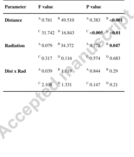
Table 1: Results of ANOVA for the effects of shooting distance, radiation level and their

interaction on the density distribution of the surface temperature excess used in Fig. 4.

Temperature distributions were obtained from TIR images taken with the mobile TIR camera

at various distances for the 1-m2 thermal test card in the laboratory and in the green wall

environments (A. and B. respectively), of the whole surface of the green wall (C.) and of the

whole surface of the wood edge (D.). Values in bold indicates significance (P<0.05).

Parameter F value P value

Distance A 0.761 B 49.510 A 0.383 B <0.001 C 31.742 D 16.843 C <0.005 D <0.01 Radiation A 0.079 B 34.372 A 0.778 B 0.047 C 0.317 D 0.116 C 0.574 D 0.683 Dist x Rad A 0.039 B 1.119 A 0.844 B 0.29 C 2.108 D 1.331 C 0.147 D 0.21

26

Figure captions:

Figure 1: RGB images (A.1, B.1, C.1) and TIR images (A.2, B.2, C.2) of the 1 m2 thermal

test card placed in the three environments (laboratory A., green wall B. and wood edge C.) –

Photos credits: Emile Faye (IRD) and Sylvain Pincebourde (CNRS).

Figure 2: Scatter plots of the thermal indices' deviation between the mobile and the fixed TIR

cameras' images of the 1 m2 thermal test card under various levels of solar radiation against the ∆ Distance (m) – the distance between the two TIR cameras (mobile minus fixed).

Negative values indicate that the metric is under-estimated by the mobile camera. (A) ∆ T mean (K), (B) ∆ SD (K), (C) ∆ Patch richness and (D) ∆ Aggregation (%). Red squares are

the indoor TIR shootings at radiation level 65 W/m². Solar radiation varied from 242 W/m2 to

915 W/m2 in the outdoor green wall environment. Standard deviation of the solar radiations is

indicated in brackets.

Figure 3: Scatter plots of thermal indices' deviation between the mobile and the fixed TIR

cameras' images of the 1 m2 thermal test card in the green wall environment, and of the 1 m2 vegetation surface in the green wall and wood edge environments, against the ∆ Distance (m)

– distance between the two TIR cameras (mobile minus fixed). (A) ∆ T mean (K), (B) ∆ SD

(K), (C) ∆ Patch richness, and (D) ∆ Aggregation. Solar radiation was 890 ±133 W/m2

for all

points.

Figure 4: Frequency distribution of the surface temperature excess (K) obtained from TIR

images of the mobile TIR camera at various distances for the 1 m2 thermal test card in the

laboratory and in the green wall environments (A. and B. respectively), of the whole surface

of the green wall (C.) and of the whole surface of the wood edge (D.) under clear sky

27

from TIR images taken at 0.3 m from individual leaves of the green-wall and the wood-edge

28

Figures:

29

30

31

Figure 4

Highlights

1-We tested the effect of increasing shooting distance on thermal metrics in thermography

2-Surface temperatures were underestimated when increasing shooting distance

3-Effect of distance on thermal metrics was stronger in the first 20 m

4-Infrared images were thermally homogenized when increasing shooting distance