HAL Id: hal-02165453
https://hal.archives-ouvertes.fr/hal-02165453
Preprint submitted on 25 Jun 2019
HAL is a multi-disciplinary open access
archive for the deposit and dissemination of sci-entific research documents, whether they are pub-lished or not. The documents may come from teaching and research institutions in France or abroad, or from public or private research centers.
L’archive ouverte pluridisciplinaire HAL, est destinée au dépôt et à la diffusion de documents scientifiques de niveau recherche, publiés ou non, émanant des établissements d’enseignement et de recherche français ou étrangers, des laboratoires publics ou privés.
Public debt versus Environmental debt: What are the
relevant Tradeoffs?
Mohamed Boly, Jean-Louis Combes, Pascale Combes Motel, Maxime Menuet,
Alexandru Minea, Patrick Villieu
To cite this version:
Mohamed Boly, Jean-Louis Combes, Pascale Combes Motel, Maxime Menuet, Alexandru Minea, et al.. Public debt versus Environmental debt: What are the relevant Tradeoffs?. 2019. �hal-02165453�
Public debt versus Environmental debt:
What are the relevant Tradeoffs?
✩Mohamed Bolya, Jean-Louis Combesa, Pascale Combes-Motela, Maxime Menueta,1,
Alexandru Mineaa,b, Patrick Villieuc
aUniversité Clermont Auvergne, CERDI, CNRS, IRD, F-63000 Clermont-Ferrand, France. bDepartment of Economics, Carleton University, Ottawa, Canada
cUniv. Orléans, CNRS, LEO, UMR 7322, FA45067, Orléans, France
Abstract
The article explores the relationship between public debt and environmental debt. The latter is defined as the difference between the "virgin state" which is the maximum stock of environmental quality that can be kept intact with natural regenerations and the current quality of the environment. A theoretical model of endogenous growth is built. We show that there is a unique well-determined balanced-growth path. The public debt and the environmental debt are substitute in the short-run but complementary in the long-run. Indeed, budget deficit provides additional resources to finance pollution abatement spending, but generate also unproductive expenditures (the debt burden). This hypothesis is tested on a sample of 22 countries for the period 1990-2011. The environmental debt is measured by the cumulative CO2 emissions per capita. We use
panel time-series estimators which allow for heterogeneity in the slope coefficients between countries. It appears mainly that, in the long term, an increase of 100% in public debt ratio leads to an increase of 74% in cumulative CO2 per capita. In addition, this positive
long-run relationship is still present at the country and the sub-sample level, despite some differences in the short-term dynamics.
Keywords: environmental debt, public debt, heterogenous panel data model JEL codes: O44, Q52, Q58
1. Introduction
Sustainable development has long been considered being backed on three pillars. Re-cent history, however, shed light on two distinguishing features of unsustainable devel-opment. They stem from global environmental degradation and especially from climate change and rising sovereign indebtedness. On the one side, energy-related CO2 emissions
rose a historic high of 33.1 Gt CO2 in 2018 (International Energy Agency, 2019). This
raised once more the issue of the environmental i.e. climatic debt that will be borne by future generations (Azar and Holmberg,1995) with a major shift in responsibilities from developed to developing countries (Botzen et al., 2008). On the other side, indebted-ness has been soaring, especially in the aftermath of the 2007-2008 crisis. Fast increase
✩This is a preliminary draft. Please do not cite or distribute without permission of the authors. 1Corresponding author: maxime.menuet@univ-orleans.fr
in public indebtedness is seen as “the most enduring legacies of the 2007-2009 financial crises” especially when it comes as a major impediment to economic growth (Reinhart and Rogoff, 2010; Eberhardt and Presbitero, 2015). Several authors, therefore, urged for both reforms of the fiscal and financial systems, which are deemed to prompt the right incentives to green growth (Aglietta and Hourcade, 2012). This is all the more necessary in the face of increasing concerns on the ability of NDCs, even if fully imple-mented, to meet the climate targets agreed in the 2015 Paris Agreement. For instance, promoting renewable energy is the most common mitigation strategy while agriculture and transport are seldom considered as key sectors for mitigation though, along with en-ergy and industry, they are the largest contributors to GHG emissions (Pauw et al.,2018). This paper contributes to the sparse literature on the interaction between environmen-tal and macroeconomic policies while scrutinizing the relationship between sovereign and environmental debt.2 One could argue that higher public indebtedness is legitimate for
financing investments in low-carbon technologies or environmental R&D activities which will mainly benefit to future generations. This assertion can, however, be challenged when the government has run deficits for many years. Hence, one can wonder about the consequences of public debt stabilization on environmental policies and outcomes. Under the assumption that public debt initiates additional pressure on the environment, debt for nature swaps can generate positive environmental outcomes. This possibility has been explored in the case of deforestation.3 It can also be argued that debt servicing crowds
out private expenditures that can entail abatement expenditures. Fodha and Seegmuller
(2014) show that public abatement partly financed by debt emission may even lead the economy to an environmental poverty trap under a stabilizing debt constraint.
This paper theoretically and empirically explores further the interdependencies be-tween environmental and sovereign debt in a long term perspective. In Section 3, relax-ing the balanced-budget rule assumption, a simple endogenous growth model establishes a complement effect between public and environmental debt along the balanced growth path of the economy. Unproductive public expenditures, i.e. the debt burden, crowd out pollution abatement expenditures. Relying on cumulative per capita consumption-based CO2 emissions as a proxy of environmental debt in Section 4, our results show that
in 22 countries increasing the debt-to-output ratio has a statistically and economically significant impact on the environmental debt in the long run.
2See for a brief review e.g. (Combes et al.,2015).
3Kahn and McDonald(1995) provided econometric support for this hypothesis while Cassimon et al.
2. The model
We consider a simple continuous-time endogenous-growth model with a representative individual, who consists of a household and a competitive firm, and a government. All agents are infinitely-lived and have perfect foresight.
2.1. Environmental debt
In the economy, environmental quality (Qt) determines nature’s capacity to grow and
absorbs wastes from economic activity. Following Tahvonen and Kuuluvainen(1991) and
Bovenberg and Smulders (1995), the evolution of environmental quality, or equivalently the evolution of the stock of environmental goods is modeled as a renewable resource
˙
Qt = E(Qt)− Pt, (1)
where a dot over a variable represents a time derivative.
In Eq. (1), Pt represents reduction in environmental quality, or natural resources,
from the net flow of emissions (say pollution), and E(·) is an environmental regeneration function and reflects the capacity of the environment to absorb pollution. We consider several standard assumptions.
Assumptions. (i) E(Qt)∈ C1(R+)
(ii) E′(Q
t) < 0 (the law of entropy )
(iii) there is a critical level ¯Q > 0, such that E( ¯Q) = 0 (virgin state)
Assumption (i) states that the regeneration process is a smooth function. Assump-tion (ii) means that the higher the stock of natural resources, the higher the difficulties to maintain or increase this stock through natural regeneration processes (which is an impli-cation of the entropy law from physics, see Smulders,1995). Assumption (iii) states that, without pollution (Pt = 0), environmental quality reaches its highest possible (finite) level
– the “virgin state” ¯Q– which is the maximal stock of natural resources that can be kept intact by natural regeneration. However, this virgin-state cannot be sustained, because economic activity incurs polluting emissions; namely the production process uses inputs (Zt) that pollute the environment, such as, e.g., pesticides in agriculture, fossil fuels
re-sulting in emissions of carbon. Such adverse effect of production can be (at least partially) neutralized by abatement spending. As usual, we assume that this abatement activity is provided by the public sector through governement’s expenditure (Gt). Consequently,
the net flow of emission is
Pt = ! Zt Gt "µ , (2)
where µ > 0 measure the elasticity of emissions to the polluting input.4
We define the gap between the virgin-state stock and the current environmental qual-ity as the environmental debt (Dt), namely
Dt = ¯Q− Qt. (3)
In the long-run, would the economy reach the virgin state (Q∗ = ¯Q, where a star
denotes steady-state values), the environmental debt would be zero (D∗ = 0). Owing
to economic activity, however, environmental quality is perpetually damaged, such that Qt < ¯Q, even in the long-run. We can then define the gap ¯Q− Qt as the obligations of
the ecosystem towards nature. 2.2. Households
The representative household starts at the initial period with a positive stock of capital (K0), and chooses the path of consumption {Ct}t≥0, and capital {Kt}t>0, so as to
maximize the present discount value of its lifetime utility U =
# ∞
0
e−ρtu(Ct, Qt) dt, (4)
where ρ ∈ (0, 1) the subjective discount rate. The instantaneous utility is assumed to be separable
u(Ct, Qt) = log(Ct) + η log(Qt),
where η > 0 captures environmental preferences.
The household enters period t with initial (predetermined) stocks of private capital (Kt) and government bonds (Bt), whose returns are respectively qt (the rental rate of
capital) and rt (the real interest rate). He perceives wages (wtL), pays taxes (where
τw ∈ (0, 1) is the proportional wage income tax rate), and decides how much to consume
(Ct) and save during the period. The only forms of asset accumulation are capital ( ˙Kt, we
omit capital depreciation, without loss of generality) and government bonds ( ˙Bt); hence
the following budget constraint ˙
Kt + ˙Bt = rtBt+ qtKt+ (1− τw)wtL− Ct. (5)
The first-order conditions give rise to the familiar Euler equation (with qt = rt in
competitive equilibrium) ˙ Ct Ct = rt− ρ, (6) 4Z
tis the flow of effective pollution, which depends both on emissions and on the abatement spending:
Zt= Pt1/µGt. Thus, the same Zt can be achieved with less emissions if the economy has access to more
abatement. The exponent µ denotes a pollution-conversion parameter: a lower µ makes pollution more effective, or equivalently, makes abatement relatively less effective.
and the optimal path must verify the set of transversality conditions lim
t→+∞{exp(−ρt) Kt/Ct} = 0 and limt→+∞{exp(−ρt) Bt/Ct} = 0,
which ensure that lifetime utility U is bounded. 2.3. Firms
Output of the representative firm (Yt) is produced using three inputs: a man-made
private capital (Kt), labor (Lt), and a polluting input (Zt), according to the following
Cobb-Douglas production function
Yt = ˜AKtαZtβ( ¯KtLt)1−α−β, (7)
where α ∈ (0, 1) and β ∈ (0, 1) are the elasticity of output to the private capital and polluting input, respectively. ˜A > 0 is a scale parameter, and Kt is the economy-wide
level of capital that generates positive technological spillovers onto firms productivity (Romer, 1986).
The firm i chooses private factors (Kt, Lt and Zt) to maximize its profit
Πt = Yt− rtKt − wtLt− τpZt,
where τpis a constant environmental tax on the polluting input. The first-order conditions
give rise to rt = α Yt Kt , (8) wt = (1− α − β) Yt Lt . (9) τp = β Yt Zt . (10)
with, at equilibrium, Lt = L. We henceforth normalize L = 1. The production function
(7) depicts a constant return-to-scale technology relative to private factors (rival inputs); hence constant output-shares of each factor.
2.4. The government
The government provides abatement public expenditures Gt, receives taxes on labor
income (τw) and on the polluting input (τp), and borrows from households. Fiscal deficit
is financed by issuing debt ( ˙Bt); hence, the following budget constraint
˙
Bt = rtBt + Gt− τpZt− τwwt. (11)
To study the relationship between environmental debt and public debt we need to escape from the balanced-budget rule hypothesis, even in the long-run. To this end, we
introduce the possibility that public deficits are permanently financed by public debt accumulation.5 At this stage the model is not closed, because there is one free variable
in the government budget constraint (11). To close the model, the government must fix either the public abatement spending or the public debt path. In our endogenous growth setup, public spending is an endogenous variable, so we consider that the public debt path follows a simple rule that links the debt-to-output ratio (bt := Bt/Yt) to a long-run
target (θ), namely6
˙bt = η(θ− bt), (12)
where η > 0 is the speed of adjustment of the debt ratio to its long-run value. This rule serves our purpose for two reasons. First, it reflects stylized facts: many fiscal rule implemented since the 1980s require an exogenous target of debt-to-output ratio (see IMF, 2017).7 Second, it allows assessing the effects of the target θ on the time profile of
environmental debt. 3. Equilibrium
At symmetric equilibrium, we have ¯Kt = Kt, and using (7),
Yt = AKt,
where A := [ ˜A(τpβ)β]1/(1−β). Thanks to constant-returns at the social level, endogenous
growth can emerge, despite decreasing returns of private capital from the individual firm’s perspective. Therefore, using (8), the real interest rate becomes
rt = αA. (13)
To obtain long-run stationary ratios, we deflate variable by output and we use lower-case characters to depict ratios, namely: ct := Ct/Yt, gt := Gt/Yt.
The path of the capital stock is given by the goods market equilibrium ˙
Kt
Kt
= A(1− gt− ct). (14)
The government’s budget constraint (11) leads to gt = η(θ− bt) +
˙ Kt
Kt
bt+ β + τw(1− α − β) − αAbt. (15)
5Effectively, many papers show that endogenous growth setups are compatible with the existence of
a growing public debt in the long-run (Minea and Villieu,2012;Boucekkine et al.,2015;Menuet et al.,
2018). The only requirement for the transversality condition to be verified is that the rate of growth of public debt must be less than the real interest rate at equilibrium.
6Another way is to assume a deficit rule, as discussed in Menuet et al.(2018). 7Such as, e.g., θ = 60% in the Maastricht treatise.
hence, gt = 1 1 + Abt [λ + η(θ− bt) + Abt(1− ct− α)], (16) where λ := β + τw(1− α − β).
From (10), it follows that Zt/Yt = τp/β. Using (1), (2) and (3), the law of motion of
the environmental debt then writes ˙ Dt = ! τp βgt "µ − E(Qt). (17)
From (6), (13), (14), and (17), the reduced-form of the model is ⎧ ⎪ ⎪ ⎪ ⎪ ⎪ ⎪ ⎪ ⎪ ⎪ ⎨ ⎪ ⎪ ⎪ ⎪ ⎪ ⎪ ⎪ ⎪ ⎪ ⎩ ˙bt = η(θ− bt), ˙ct ct = C˙t Ct − ˙ Kt Kt = αA− ρ − A 1 + Abt (1− ct− λ − η(θ − bt) + αAbt) , ˙ Dt = ! τp βgt "µ − E( ¯Q− Dt). (18) 3.1. Steady state
We define a balanced-growth path (BGP) as a path on which consumption, capital, output, and public debt grow at the same (endogenous) rate, namely (we henceforth omit time indexes)
γ∗:= ˙C/C = ˙K/K = ˙Y /Y = ˙B/B,
and environmental debt is constant ( ˙D = 0). The following proposition computes the steady-state by setting ˙c = ˙b = ˙D = 0 in system (18).
Proposition 1. (Existence and Uniqueness) If ρ < min(αA, λ/θ), there is a unique BGP with positive economic growth, environmental debt, and consumption and public spending ratios.
Proof: Using (6) and (13), the long-run economic growth rate is γ∗ = αA − ρ, which
is positive under the mild condition A > ρ/α (that is verified for small discount rate). From (15.b), the public debt ratio reaches its long-run target, i.e. b∗ = θ. Using (15.a),
˙c = 0 leads to 1− c∗ = (αA −ρ)(1+θA)
A − αAθ + λ, hence,
c∗ = (1− τw)(1 + β− α) + ρ(1 + θA)/A > 0. (19)
From (16), we derive
which is positive as ρ is small. Finally, using (15.c), at the steady state, the environmental debt ratio D∗ is D∗= ¯Q− E−1 !! τp βg∗ "µ" > 0. (21) ! To complete the characterization of the equilibrium, we must ensure that the unique BGP is well determined, i.e. saddle-path stable, as state the following proposition. Proposition 2. (Stability) The unique BGP is saddle-path stable (well-determined). Proof : By linearization, in the neighborhood of steady state, the system (18) behaves according to (˙bt, ˙ct, ˙Dt) = J(bt − b∗, ct − c∗, Dt − D∗), where J is the Jacobian matrix.
As the reduced-form includes one jump variable (the consumption ratio c0) and two
pre-determined variables (the environmental debt D0 and the public-debt ratio b0 = B0/AK0,
since initial levels of public debt and capital are predetermined), for the BGP to be well determined, J must contain two negative and one positive eigenvalues. Using (18), we compute J = ⎛ ⎜ ⎝ −η 0 0 CB CC 0 DB DC E′(·) ⎞ ⎟ ⎠
where CC = c∗A/(1 + θA) > 0. As J is a triangular matrix, the eigenvalues are:
λ1 =−η < 0, λ2 = CC > 0 and λ3 = E′(·) < 0. !
Proposition 2 states that the model is locally well determined. From any pre-determined values b0 and D0, the initial consumption ratio (c0) jumps to put the economy on the
unique saddle path that converges towards the BGP. The following subsection addresses the relationship between the public debt ratio and the environmental debt in the short-run and the long-run.
3.2. Environmental Debt vs Public Debt
Based on the preceding dynamics analysis, the following proposition establishes the main result of the theoretical section by assessing the effect of changes in the public-debt target (θ) on public debt (bt) and environmental debt (Dt).
Proposition 3. Following a change in the debt target (θ), public debt and environmental debt are (i) complement in the long-run, and (ii) substitute in the short-run, provided that b0 < b0 := η/Aρ.
Proof : From (20), in the long-run (b∗ = θ), we observe that ∂g∗/∂θ < 0. At the
ini-tial time, the consumption ratio immediately jumps to its steady-state value (c0 = c∗).
Consequently, from (21), we have ∂D∗/∂θ > 0, since sgn(∂D∗/∂θ) = −sgn(∂g∗/∂θ). At
the initial time, using (18), it follows that ∂ ˙D0/∂θ = −µ(D0/g0)∂g0/∂θ < 0. As D0 is
predetermined, there is ¯t > 0, such that Dt < D0, ∀t ∈ (0, ¯t). !
Proposition 4 reveals that the time profile of environmental debt basically depends on the behavior of government abatement spending. An increase in the debt target gen-erates new deficit that produces two opposite effects: there are (i) a permanent flow of new resources for abatement activity ( ˙Bt), and (ii) a permanent flow of new
unproduc-tive expenditures (the debt burden rtBt). In the long-run, the transversality condition
(r∗ > γ∗ = ˙B/B∗⇔ r∗B∗> ˙B) means that the latter dominates the former, hence public
debt has an adverse effect on abatement expenditure in steady-state. In the short-run, in contrast, the first effect outweighs the second, and the new deficit provides additional re-sources for abatement (net from the debt burden). Provided that b0 < b0, these resources
serve to increase environmental quality, reducing the ecological debt.
Figure 1 illustrates the behavior of environmental debt (the upper graph) and the public debt ratio (the lower graph) for a baseline calibration8, following an increase in
the debt target from θ = 50% to θ = 100%. We observe that the two variables are substitute until ¯t = 40, and complement from ¯t onward.
Figure 1: Dynamic adjustment of environmental debt and public debt following an increase in θ
4. Empirical Methods 4.1. Data
Environmental Debt. We rely on cumulative carbon emissions to measure envi-ronmental debt. We calculate cumulative historical carbon emissions, using annual data from the Global Carbon Project. We use consumption-based emissions which have the advantage of incorporating emissions from international transportation as well as carbon leakages. The data are available from 1990 and are measured in million tonnes of carbon (MtC)9. We convert annual carbon emissions in tonnes of CO
2 before reporting them to
population. Thus, the environmental debt for country i at year t is given by Dit =
t
.
j=1990
(CO2i)j
Where CO2 stands for per capita CO2 emissions. We take the natural logarithm of Dit
for the econometric analysis.
Public Debt. Data on Gross public debt come from the IMF Historical Public finance dataset which is used in Mauro et al. (2015) and which goes back far into the past. Public debt is measured in percent of GDP. The data on debt-to-output ratio go up to the year 2011 for each country, therefore limiting our maximum time period length to 22, when combined to emissions data which start from 1990. Moreover, there were some gaps for both variables in some countries; since our sample consists in high income and upper-middle income countries10 and because of data limitations, we end up with
a balanced panel of 22 countries over the period 1990-2011. Summary statistics of our variables, as well as the list of countries, are reported in appendix B.
4.2. Methodology
In line withPesaran et al.(1999), let’s assume an autoregressive distributed Lag model (ARDL), with p lags for Environmental debt and q lags for our RHS variable, namely public debt LogDit = p . j=1 αijLogDi,t−j+ q . j=0 δ′ijθi,t−j+ µi+ ϵit, (22)
with i = 1, N countries, t = 1, T periods, D environmental debt, θ the debt-to-output ratio, µi country-specific effects, and ϵit the error term. If we assume that the variables
91MtC= 3.664 million tonnes of CO 2
10Income groups defined according to the World Bank definition. We also consider CO
2 emissions as
an issue of less importance in developing countries, which motivates our choice to work on countries of the upper-middle and high income groups.
are I(1) and cointegrated, equation 12 can be reparameterized into the following error correction model (Pesaran et al., 1999)
∆LogDit= Φi(LogDi,t−1− β ′ iθit) + p−1 . j=1 α∗ij∆LogDi,t−j+ q−1 . j=0 δ∗ij′∆θi,t−j+ µi+ ϵit, (23) where Φi =−(1− p . j=1 αij), βi = q . j=0 δij/(1− . k αik), α∗ij =− p . m=j+1 αim, and δ∗ij =− q . m=j+1 δim.
The second part in differences of Eq. (23) illustrates the short-run adjustment to the long-run equilibrium, while the first part- in levels- captures the long-run relationship. The speed of adjustment is given by the error-correcting term φi, which should be negative
and significant to validate the presence of a long-run relationship.
There are three main approaches in the literature to estimate Eq. (23): (i) the dynamic fixed effects estimator (DFE) that allows only different intercepts across units but which turns out to be inconsistent if the common slope assumption fails to hold; (ii) the pooled mean group estimator (PMG) which assumes common long-run coefficients across units while allowing short-run coefficients to differ across units, and (iii) the mean group estimator (MG) which allows slope coefficients, intercepts and errors variances to be different across groups (Pesaran and Smith,1995).
We start using the DFE estimator in a first stage, since we are interested in capturing long-run dynamics, and further use the PMG estimator to also assess the short-run dy-namic while still controlling for the long-run relationship between our variables. Following AIC, we use an ARDL(1,1) meaning that we set p = 1 and q = 1 in Eq. 12.
4.3. Results
4.3.1. Stationarity and cointegration
To assess the stationarity of our variables, we rely on the Fisher-ADF and IPS unit root tests. The results are reported in Table 1. In the auto-regressive specification of each test we include both the trend and the intercept and we remove cross-sectional means to mitigate the effects of cross-sectional correlation. As we see in table 1, irrespective of the test, we cannot reject the null hypothesis of the presence of a unit root for our variables. Moreover, we also see that there are stationary in first-difference, meaning that there are I(1). Since they are integrated of the same order, we therefore look for potential cointegration relations among them.
For this purpose, we draw upon Westerlund (2007)’s tests. In these tests, the null hypothesis of no cointegration is assumed against four different specifications of the alter-native hypothesis: the group mean test and its asymptotic version, that both consider the
Table 1: Unit root tests
Variables ADF IPS
Statistic p-value Statistic p-value Log(Environmental Debt) Z: 1.65 0.95 W-T-bar: 1.38 0.92
Pm: -0.05 0.52
∆(Log Environmental Debt) Z: -7.60 0.00 W-T-bar: -6.63 0.00 Pm: 13.68 0.00
Gross Public Debt Z: 2.31Pm: -1.04 0.99 W-T-bar: 2.680.85 0.99 ∆(Gross Public Debt) Z: -2.21 0.01 W-T-bar: -5.26 0.00
Pm: 2.79 0.00
Note: Pm represents the modified inverse chi-squared and Z is the inverse normal statistic. The null hypothesis is "all panels contain unit roots". We use 1 lag following AIC. We include both trend and intercept.
alternative assumption that there is cointegration for the panel as a whole, and the panel mean test with its asymptotic version, which consider that the variables are cointegrated for at least one cross-section unit in the alternative assumption. We carry out these tests using bootstrap with 400 replications, in order to preserve size accuracy as well as consistency in the case of cross-sectional dependence. The results of testing a potential cointegration between environmental debt and public debt are provided by table 2. The low p-values support the presence of cointegration between our variables in level.
Table 2: Westerlund (2007) cointegration tests
Statistic Value Z-value P-value
Gt -6.223 -18.384 0.000
Ga -47.487 -20.205 0.000
Pt -10.324 -2.450 0.007
Pa -31.742 -14.408 0.000
Note: Gt and Pt correspond respectively to the group mean test and the panel mean test. Ga and Pa are their respective asymptotic versions. The null assumption is "no cointegration". 3 lags determined by AIC.
Since they are I(1) and co-integrated, in the following we draw upon an error correction model to assess the effect of public debt on environmental debt.
4.3.2. Public Debt and Environmental Debt: Full sample
Table 3 reports the results of the error correction model; the first column presents the results of the dynamic fixed effects (DFE) estimator. The error correction term is negative and significant, thus justifying our modelling choice.
common long-run and short-run dynamics for all countries. The assumption of a common run dynamic seems unrealistic, insofar as the increase of public debt in the short-run, resulting from higher expenditure, does not necessarily lead to the same level of abatement expenditure among countries with different environmental policies. However, for the long-run, it is possible to assume a common path since an increase in public debt leads to lower spending, including abatement expenditure, which in turn results in higher environmental debt.
Table 3: Environmental Debt response
Dependent Variable Log (Environmental Debt)
DFE PMG
Error correction term -0.180∗∗∗ -0.193∗∗∗
(0.0033) (0.0061) Long run coefficients
Gross public debt 0.0028∗∗ 0.0074∗∗∗
(0.0011) (0.0004) Short run coefficients
∆(Gross public debt) -0.0009∗∗∗ -0.0017∗∗
(0.0003) (0.0007) Constant 0.844∗∗∗ 0.840∗∗∗ (0.0112) (0.0341) Observations 462 462 Countries 22 22 Log likelihood 724
Hausman Test p-value 0.5246
Standard errors in parentheses
∗p < 0.10,∗∗p < 0.05,∗∗∗p < 0.01
We therefore decide to allow for different short-run dynamics while still assuming a common long-term path: to do so we rely on the Pooled Mean Group (PMG) estimator, which results are presented in column 2 of table 3. We test its common long-term co-efficient assumption against the alternative hypothesis of different coco-efficients, using the Hausman Chi-2 test which p-value is reported in the bottom of table 3. Since we are not rejecting the null hypothesis of a common long-run path for countries in our sam-ple (p-value=0.5246), we keep the specification using the PMG as our baseline for the following.
The error correction term is also negative and significant, and the results in column 2 are consistent with our theoretical predictions: more public debt results in higher environmental debt in the long run. To illustrate, an increase of 100 units in the debt-to-output ratio leads to an increase of 74% in cumulative per capita CO2 in the long-run.
More public debt leads to higher environmental debt in the long run, since it implies lower abatement expenditure in the long run. But in the short run, since higher public debt
is linked to higher expenditure, we have a negative effect on cumulative CO2 because of
higher abatement expenditure. We see that a 100 units increase in public debt leads to a reduction of 17% in cumulative emissions.
4.3.3. Public Debt and Environmental Debt: country evidence
Beyond full sample estimates, it could also be interesting to look at country estimates of the short-run impact of public debt, given that it might differ across countries. Thus, using PMG estimates from table 3, we report short-run impacts for each country in table 4 and table 5. Regarding sign differences, most of our short-run coefficients are negative even though many of them are non-significant. We even have a positive effect in United States, suggesting a positive short-run relationship between public debt and environmental debt in this country.
Table 4: Heterogeneity in short-run coefficients
Short run coefficients by country Long run Argentina Austria Brazil China Colombia Finland France Germany Greece Italy Japan
Public Debt 0.0074***
0.0004 Error correction term -0.1979*** -0.1775*** -0.1943*** -0.1563*** -0.2126*** -0.1655*** -0.2099*** -0.1968*** -0.1997*** -0.1724*** -0.3042***
0.0206 0.0155 0.0138 0.0168 0.0126 0.0218 0.0165 0.0151 0.0155 0.0174 0.0130 ∆(Public Debt) -0.0013** -0.0028 -0.0019 -0.0011 -0.0054** 0.0026 -0.0022 -0.0052 -0.0004 0.0019 -0.0016* 0.0005 0.0052 0.0016 0.0033 0.0025 0.0029 0.0039 0.0033 0.0015 0.0033 0.0008 Constant 0.7202*** 0.8764*** 0.5910*** 0.6184*** 0.6652*** 0.8909*** 0.9568*** 1.0016*** 0.8682*** 0.7688*** 1.2242*** 0.0614 0.0652 0.0325 0.0504 0.0319 0.1020 0.0653 0.0657 0.0569 0.0663 0.0333 Observations 462 Countries 22 Log likelihood 724
Table 5: Heterogeneity in short-run coefficients (continued)
Short run coefficients by country Long run Korea, Rep. Norway Portugal Romania Spain Switzerland Thailand Turkey Un. Kingdom United States Uruguay
Public Debt 0.0074***
0.0004 Error correction term -0.1804*** -0.2048*** -0.1892*** -0.1781*** -0.1738*** -0.2006*** -0.1887*** -0.1898*** -0.1913*** -0.1841*** -0.1756***
0.0132 0.0137 0.0140 0.0186 0.0168 0.0170 0.0142 0.0198 0.0153 0.0126 0.0148 ∆(Public Debt) -0.0074 -0.0033 0.0026 0.0006 -0.0012 -0.0080** -0.0031** -0.0023 0.0005 0.0040* -0.0020** 0.0064 0.0021 0.0024 0.0030 0.0025 0.0033 0.0015 0.0017 0.0025 0.0021 0.0009 Constant 0.9263*** 0.9741*** 0.8182*** 0.7986*** 0.7988*** 1.0063*** 0.7004*** 0.7358*** 0.9528*** 0.9890*** 0.5943*** 0.0543 0.0562 0.0485 0.0711 0.0646 0.0738 0.0412 0.0635 0.0648 0.0589 0.0383 Observations 462 Countries 22 Log likelihood 724
We also find differences in terms of magnitude across short-run impacts: for instance, the short-run negative effect for Switzerland is four times more important than the Uruguay’s. These findings shed light on possible short-run heterogeneities across our sample: for some countries, the results are in line with the theoretical predictions of sub-stitution in the short run and complementarity in the long-run between the two debts. However, for some countries, we find no significant impact for the short-run relationship. Even more, for a country like United States, we find a positive relation suggesting that more public debt does not necessary lead to higher abatement expenditure in the short run.
Thus, even if we expect countries in our sample to converge toward a common steady state in the long run, one could assume that the short-run dynamic of their environmental
debt can differ. Such findings invite us to explore more closely particularities at play in our sample.
4.3.4. Public Debt and Environmental Debt: conditionality upon structural characteristics Short-run differences we emphasized in the previous section could be linked to coun-tries’ economic and structural differences. Thus, in the following the analyze the sen-sitivity of our short-run coefficients to such differences. We consider four structural characteristics; first we capture differences in terms of environmental preferences through income (Grossman and Krueger,1995) by considering alternatively upper-middle income and high income countries. Second, we also consider the fiscal stance and so the leeway in terms of public debt, using the average debt to GDP ratio over the period. We take a 60% threshold (as suggested by the Maastricht Treaty) to split countries.
Third, we take the openness degree into account through average trade in percentage of GDP; we therefore split our countries into groups with relatively low and high openness, based on the sample median. Finally, we also look at the average environmental debt over the period 11 and we use its sample median to divide the sample into countries with
low and high environmental debt. Tables in appendix B present descriptive statistics and the countries for each group.
Table 6: Environmental Debt response (conditionality upon structural characteristics)
Dependent Variable Log(Environmental Debt)
Full Sample Income group Public Debt Openness Env. Debt
Upper-Middle High Low High Low High Low High
Error correction term -0.193∗∗∗ -0.189∗∗∗ -0.195∗∗∗ -0.186∗∗∗ -0.203∗∗∗ -0.198∗∗∗ -0.188∗∗∗ -0.180∗∗∗ -0.197∗∗∗
(0.0061) (0.0079) (0.0079) (0.0043) (0.0150) (0.0108) (0.004) (0.0057) (0.0094) Long run coefficients
Gross public debt 0.0074∗∗∗ 0.0084∗∗∗ 0.0073∗∗∗ 0.0069∗∗∗ 0.0074∗∗∗ 0.0073∗∗∗ 0.0081∗∗∗ 0.0039∗∗∗ 0.0076∗∗∗
(0.0004) (0.0022) (0.0004) (0.0017) (0.0004) (0.0004) (0.0025) (0.0014) (0.0004) Short run coefficients
∆(Gross public debt) -0.0017∗∗ -0.0023∗∗∗ -0.0015∗ -0.0024∗∗∗ -0.0004 -0.0011∗ -0.0024∗∗ -0.0018∗∗∗ -0.0015
(0.0007) (0.0008) (0.0009) (0.0008) (0.0011) (0.0007) (0.0012) (0.0006) (0.001) Constant 0.840∗∗∗ 0.684∗∗∗ 0.898∗∗∗ 0.802∗∗∗ 0.908∗∗∗ 0.794∗∗∗ 0.892∗∗∗ 0.685∗∗∗ 0.932∗∗∗ (0.0341) (0.0314) (0.0358) (0.0404) (0.0569) (0.0545) (0.0312) (0.0269) (0.0311) Observations 462 126 336 294 168 252 210 168 294 Countries 22 6 16 14 8 12 10 8 14 Log likelihood 724.0 192.9 531.2 445.9 278.2 400.7 323.3 253.2 473.1
Standard errors in parentheses
∗p < 0.10,∗∗p < 0.05,∗∗∗p < 0.01
Table 6 presents the results obtained for the different country groups. As we can see, the positive long-run relationship between our variables remains robust among the different sub-samples. Concerning the magnitudes of the long-run coefficients, we find no significant differences between the sub-groups for income, public debt and openness.
11It its worth to mention that since we are considering averages, some of the biggest contemporary
polluters like China could appear in the group of countries with low environmental debt. This because their emissions started increasing strongly only over recent periods; moreover, environmental debt is calculated using consumption-based emissions rather than production-based emissions.
These coefficients are very similar to the long-run impact we found for whole sample. However, we find that the long-run effect for countries with an important environmental debt is about twice the one we obtain for countries with a low environmental debt. As in the baseline result, we also find negative and significant short-run coefficients for most of the sub-samples, except for countries with high levels of debt, both public and environmental.
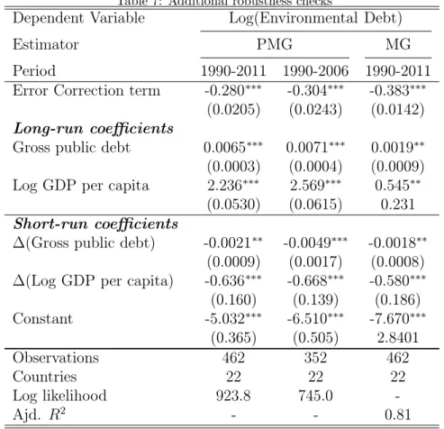
4.3.5. Additional Robustness Checks
Table7provides additional robustness checks of our relation. In the first column, we control for the level of economic activity through GDP per capita12, while in column 2
we alter our sample to remove the aftermath of the 2007-2008 crisis during which there was an important increase in public debt.
Table 7: Additional robustness checks
Dependent Variable Log(Environmental Debt)
Estimator PMG MG
Period 1990-2011 1990-2006 1990-2011
Error Correction term -0.280∗∗∗ -0.304∗∗∗ -0.383∗∗∗
(0.0205) (0.0243) (0.0142) Long-run coefficients
Gross public debt 0.0065∗∗∗ 0.0071∗∗∗ 0.0019∗∗
(0.0003) (0.0004) (0.0009) Log GDP per capita 2.236∗∗∗ 2.569∗∗∗ 0.545∗∗
(0.0530) (0.0615) 0.231 Short-run coefficients
∆(Gross public debt) -0.0021∗∗ -0.0049∗∗∗ -0.0018∗∗
(0.0009) (0.0017) (0.0008) ∆(Log GDP per capita) -0.636∗∗∗ -0.668∗∗∗ -0.580∗∗∗
(0.160) (0.139) (0.186) Constant -5.032∗∗∗ -6.510∗∗∗ -7.670∗∗∗ (0.365) (0.505) 2.8401 Observations 462 352 462 Countries 22 22 22 Log likelihood 923.8 745.0 -Ajd. R2 - - 0.81
Standard errors in parentheses
∗ p < 0.10,∗∗ p < 0.05,∗∗∗p < 0.01
To do so, we consider the period prior to 2007. Even though the Hausman test in table 3 suggests us to prefer the common long-run path assumption i.e to rely on PMG estimates, we however run a specification using Mean-group estimator in column 3. This,
to test whether its results are qualitatively different from PMG estimates. It also includes cross-sectional averages to account for potential cross-sectional dependence. The results we obtain are again similar and support the presence of a complement effect in the long-run and a substitution effect in the short-long-run.
5. Conclusion
Hartwick (1997) rightly argued that paying down the environmental debt is a si-milar process than paying down public debt: both tasks mobilize billions of dollars to be disbursed over decades to meet targets either agreed in multilateral environmental agreements or set by fiscal rules. This paper builds on this idea while theoretically and empirically showing that public debt and environmental debt are complements in the long run. Our econometric results, however, evidenced some differences in short run environmental debt dynamics. In the USA for instance, there is a positive link between environmental and public debts in the short run. Given the fact that the USA is a still major CO2 emitter, the sharp increase in the US public debt results in higher CO2
emissions in the short run. In the long run, however, our results support the idea that stricter climate policies can generate environmental benefits but can also correlate to better macroeconomic performance, as measured by debt stabilization.
Our results support the idea that, in the long run, there is no-trade-off between debt stabilization that is a major concern, especially since the 2007-2008 crisis, and environ-mental performance. Our findings can, however, have some theoretical and econometric limitations. First, we have only taken public debt and public abatement expenditures. Private debt is not accounted for despite the fact that several emerging countries already seem to exhibit high levels of private indebtedness. Second, we assumed no composi-tion effect of public expenditures. One could argue that the complementarity between environmental and public debt is conditional on the relative importance of investment and abatement expenditures. Third, we focused on global pollution as measured by cu-mulative past CO2 emissions because of data limitations. Other global environmental
degradation measures should also be taken into account, as well as local pollution with huge health consequences.
References
Aglietta, M., Hourcade, J.C., 2012. Can indebted europe afford climate policy? can it bail out its debt without climate policy. Intereconomics - Review of European Economic Policy 3, 159–64.
Azar, C., Holmberg, J., 1995. Defining the generational environmental debt. Ecological Economics 14, 7–19. doi:10.1016/0921-8009(95)00007-V.
Botzen, W.J., Gowdy, J.M., Van Den Bergh, J.C., 2008. Cumulative CO2 emissions: shifting
interna-tional responsibilities for climate debt. Climate Policy 8, 569–576. doi:10.3763/cpol.2008.0539. Boucekkine, R., Nishimura, K., Venditti, A., 2015. Introduction to financial frictions and debt
con-straints. Journal of Mathematical Economics 61, 271–275. doi:10.1016/j.jmateco.2015.10.003. Bovenberg, A.L., Smulders, S., 1995. Environmental quality and pollution-augmenting technological
change in a two-sector endogenous growth model. Journal of Public Economics 57, 369–391. doi:10. 1016/0047-2727(95)80002-Q.
Cassimon, D., Prowse, M., Essers, D., 2011. The pitfalls and potential of debt-for-nature swaps: A US-Indonesian case study. Global Environmental Change 21, 93–102. doi:10.1016/J.GLOENVCHA. 2010.10.001.
Combes, J.L., Combes Motel, P., Minea, A., Villieu, P., 2015. Deforestation and seigniorage in developing countries: A tradeoff? Ecological Economics 116, 220–230. doi:10.1016/J.ECOLECON.2015.03.029. Eberhardt, M., Presbitero, A.F., 2015. Public debt and growth: Heterogeneity and non-linearity. Journal
of International Economics 97, 45–58. doi:10.1016/j.jinteco.2015.04.005.
Fodha, M., Seegmuller, T., 2014. Environmental Quality, Public Debt and Economic Development. Environmental and Resource Economics 57, 487–504. doi:10.1007/s10640-013-9639-x.
Grossman, G., Krueger, A.B., 1995. Economic growth and the environment. Quarterly Journal of Economics 110, 353–375. doi:10.2307/2118443.
Hartwick, J.M., 1997. Paying down the Environmental Debt. Land Economics 73, 508. URL: http: //www.jstor.org/stable/3147242?origin=crossref, doi:10.2307/3147242.
International Energy Agency, 2019. Global Energy & CO2 Status Report 2018 - The Latest Trends in Energy and Emissions in 2018 URL: https://webstore.iea.org/ global-energy-co2-status-report-2018.
Kahn, J.R., McDonald, J.A., 1995. Third-world debt and tropical deforestation. Ecological Economics 12, 107–123. doi:10.1016/0921-8009(94)00024-P.
Mauro, P., Romeu, R., Binder, A., Zaman, A., 2015. A modern history of fiscal prudence and profligacy. Journal of Monetary Economics 76, 55–70. doi:10.1016/J.JMONECO.2015.07.003.
Menuet, M., Minea, A., Villieu, P., 2018. Deficit, Monetization, and Economic Growth: A Case for Multiplicity and Indeterminacy. Economic Theory 65, 819–853.
Minea, A., Villieu, P., 2012. Persistent Deficit, Growth, and Indeterminacy. Macroeconomic Dynamics 16, 267–283.
Pauw, W.P., Klein, R.J.T., Mbeva, K., Dzebo, A., Cassanmagnago, D., Rudloff, A., 2018. Beyond headline mitigation numbers: we need more transparent and comparable NDCs to achieve the Paris Agreement on climate change. Climatic Change 147, 23–29. doi:10.1007/s10584-017-2122-x. Pesaran, M., Smith, R., 1995. Estimating long-run relationships from dynamic heterogeneous panels.
Journal of Econometrics 68, 79–113. doi:10.1016/0304-4076(94)01644-F.
Pesaran, M.H., Shin, Y., Smith, R.P., 1999. Pooled Mean Group Estimation of Dynamic Heterogeneous Panels. Journal of the American Statistical Association 94, 621. doi:10.2307/2670182.
Reinhart, C.M., Rogoff, K.S., 2010. Growth in a Time of Debt. & Proceedings 100, 573–578. doi:10. 1257/aer.100.2.573.
Romer, P.M., 1986. Increasing returns and long-run growth. Journal of political economy 94, 1002–1037. Smulders, S., 1995. Entropy, environment, and endogenous economic growth. International Tax and
Public Finance 2, 319–340.
Tahvonen, O., Kuuluvainen, J., 1991. Optimal growth with renewable resources and pollution. European Economic Review 35, 650–661.
Westerlund, J., 2007. Testing for error correction in panel data. Oxford Bulletin of Economics and Statistics 69, 709–748. doi:10.1111/j.1468-0084.2007.00477.x.
Appendix A. Empirical analysis
Table B.1: Descriptive statistics
Variable Observations Mean Std. Dev. Min Max
Cumulated CO2 (tonnes per capita) 484 91.5038 80.1105 1.5847 417.2603
Gross public debt (% GDP) 484 56.2993 35.1934 1.0267 229.61
Trade (% GDP) 484 54.067 24.3395 13.7531 140.437
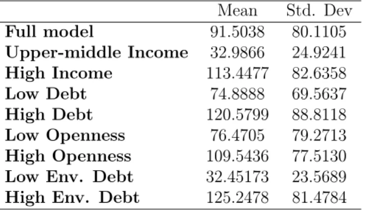
Table B.2: Summary statistics of cumulated CO2in tonnes per capita (by category)
Mean Std. Dev Full model 91.5038 80.1105 Upper-middle Income 32.9866 24.9241 High Income 113.4477 82.6358 Low Debt 74.8888 69.5637 High Debt 120.5799 88.8118 Low Openness 76.4705 79.2713 High Openness 109.5436 77.5130 Low Env. Debt 32.45173 23.5689 High Env. Debt 125.2478 81.4784
Table B.3: Summary statistics of public debt in % of GDP (by category)
Mean Std. Dev Full model 56.2993 35.1934 Upper-middle Income 31.4658 19.4508 High Income 65.6118 35.2743 Low Debt 40.3523 19.8290 High Debt 84.2065 38.7023 Low Openness 66.1645 41.5005 High Openness 44.4611 20.1304
Low Env. Debt 37.9689 25.1961
Table B.4: Summary statistics of trade in % of GDP (by category) Mean Std. Dev Full model 54.067 24.3395 Upper-middle Income 52.923 30.4532 High Income 54.496 21.6426 Low Debt 58.2233 24.6436 High Debt 46.7934 22.0468 Low Openness 38.1846 12.9786 High Openness 73.1258 20.8637
Low Env. Debt 48.9801 28.0558
High Env. Debt 56.9738 21.4485
Table B.5: List of countries
Argentina Greece Switzerland
Austria Italy Thailand
Brazil Japan Turkey
China Korea, Rep. United Kingdom Colombia Norway United States Finland Portugal Uruguay France Romania
Germany Spain
Table B.6: List of countries by characteristics
Income group Public Debt Openness Env. Debt
Upper-middle High Low High Low High Low High
Brazil Argentina Brazil Argentina Argentina Austria Argentina Austria China Austria China Austria Brazil Finland Brazil Finland Colombia Finland Colombia Germany China Germany China France Romania France Finland Greece Colombia Korea, Rep. Colombia Germany Thailand Germany France Italy France Norway Romania Greece Turkey Greece Korea, Rep. Japan Greece Portugal Thailand Italy
Italy Norway Portugal Italy Romania Turkey Japan Japan Romania United States Japan Switzerland Uruguay Korea, Rep.
Korea, Rep. Spain Spain Thailand Norway
Norway Switzerland Turkey United Kingdom Portugal
Portugal Thailand United States Spain
Spain Turkey Uruguay Switzerland
Switzerland United Kingdom United Kingdom
United Kingdom Uruguay United States
United States Uruguay