HAL Id: hal-02284339
https://hal.umontpellier.fr/hal-02284339
Preprint submitted on 11 Sep 2019
HAL is a multi-disciplinary open access
archive for the deposit and dissemination of
sci-entific research documents, whether they are
pub-lished or not. The documents may come from
L’archive ouverte pluridisciplinaire HAL, est
destinée au dépôt et à la diffusion de documents
scientifiques de niveau recherche, publiés ou non,
émanant des établissements d’enseignement et de
Emilie Joetzjer, Fabienne Maignan, Jérôme Chave, Daniel Goll, Ben Poulter,
Jonathan Barichivich, Isabelle Maréchaux, Sebastiaan Luyssaert, Matthieu
Guimberteau, Kim Naudts, et al.
To cite this version:
Emilie Joetzjer, Fabienne Maignan, Jérôme Chave, Daniel Goll, Ben Poulter, et al.. The importance
of tree demography and root water uptake for modelling the carbon and water cycles of Amazonia.
2019. �hal-02284339�
1
The importance of tree demography and root water uptake for
modelling the carbon and water cycles of Amazonia
Emilie Joetzjer
1,2, Fabienne Maignan
1, Jérôme Chave
2, Daniel Goll
1, Ben Poulter
3, Jonathan
Barichivich
1,4, Isabelle Maréchaux
2,5, Sebastiaan Luyssaert
1,6, Matthieu Guimberteau
1,7, Kim Naudts
1,8,
5
Damien Bonal
9, Philippe Ciais
11Laboratoire des Sciences du Climat et de l’Environnement, LSCE-IPSL (CEA-CNRS-UVSQ), 91190 Gif-sur-Yvette,
France
2Laboratoire Evolution et Diversité Biologique, UMR 5174, Université Paul Sabatier, CNRS, IRD, 31400 Toulouse, France
10
3 NASA Goddard Space Flight Center, Biospheric Sciences Laboratory, Greenbelt, MD, USA
4Instituto de Conservación, Biodiversidad y Territorio, Universidad Austral de Chile, Valdivia, Chile, and Center for
Climate and Resilience Research, Santiago, Chile
5 AMAP, Université de Montpellier, IRD, CIRAD, CNRS, INRA, 34000 Montpellier, France 6 Vrije Universiteit Amsterdam, Faculty of Science, 1081 HV, The Netherlands.
15
7UMR 7619 METIS, Sorbonne Universités, UPMC, CNRS, EPHE, 4 place Jussieu, 75005 Paris, France 8 Max Planck Institute for Meteorology, Bundesstraβe. 53, 20146 Hamburg, Germany
9 Université de Lorraine, AgroParisTech, INRA, UMR Silva, 54000 Nancy, France
Correspondence to: Emilie.joetzjer@lsce.ipsl.fr
Abstract. Amazonian forest plays a crucial role in regulating the carbon and water cycles in the global climate system.
20
However, the representation of biogeochemical fluxes and forest structure in dynamic global vegetation models (DGVMs) remains challenging. This situation has considerable implications for modelling the state and dynamics of Amazonian forest. To address these limitations, we present an adaptation of the ORCHIDEE-CAN DGVM, a second-generation DGVM that explicitly models tree demography and canopy structure with an allometry-based carbon allocation scheme and accounts for hydraulic architecture in the soil-stem-leaf continuum. We use two versions of this DGVM: the first one (CAN) includes a 25
new parameterization for Amazonian forest; the second one (CAN-RS) additionally includes a mechanistic root water uptake module, which models the hydraulic resistance of the water transfer from soil pores to roots. We compared the results with the simulation output of the “big-leaf” standard version of the ORCHIDEE DGVM (TRUNK) and with observations of turbulent energy and CO2 fluxes at flux tower locations, of carbon stocks and stand density at inventory plots and
observation-based models of photosynthesis (GPP) and evapotranspiration (LE) across the Amazon basin. CAN-RS 30
reproduced observed carbon and water fluxes and carbon stocks as well as TRUNK across Amazonia, both at local and at regional scales. In CAN-RS, water uptake by tree roots in the deepest soil layers during the dry season significantly improved the modelling of GPP and LE seasonal cycles, especially over the Guianan and Brazilian Shields. These results imply that explicit coupling of the water and carbon cycles improves the representation of biogeochemical cycles in Amazonia and their spatial variability. Representing the variation in the ecological functioning of Amazonia should be the 35
next step to improve the performance and predictive ability of new generation DGVMs.
1 Introduction
Amazonian rainforests store approximately half of the world’s tropical forest carbon stock (Baccini et al., 2012) and play a crucial role in global water, energy and carbon cycling (Eltahir and Bras, 1994; Werth and Avissar, 2002). The resilience and
resistance of these forests to climate change is of great concern, especially since a significant portion of Amazonia will likely experience longer and drier dry seasons by the end of the 21st century (Boisier et al., 2015; Joetzjer et al., 2013). Future
changes in the rate of carbon sequestered by Amazonia could potentially lead the global climate system to a critical tipping point (Ahlström et al., 2017; Lenton et al., 2008; Nobre and Borma, 2009), and trigger positive carbon cycle climate feedbacks from forest dieback. Yet, large uncertainties impede the production of robust future projections of changes in net 5
carbon uptake over Amazonia (Arora et al., 2013; Jones et al., 2013; Poulter et al., 2010) – current model projections range from no change, or an increase in tree biomass production (Cox et al., 2013; Huntingford et al., 2013; Rammig et al., 2010), to large-scale Amazonian dieback (Cox et al., 2004; Good et al., 2011).
An analysis of variance on simulation outputs from 12 Earth System models (ESM) showed that uncertainties in projections 10
of terrestrial carbon uptake are primarily driven by model structure (Lovenduski and Bonan, 2017). These uncertainties arise from both the atmospheric (Ahlström et al., 2012) and the land surface components (Booth et al., 2012; Sitch et al., 2015). In land models (dynamic global vegetation models, or DGVMs) large sources of uncertainty include the vegetation response to droughts (Restrepo-Coupe et al., 2016), and tree demographic processes (Fisher et al., 2010; Rödig et al., 2018). Most DGVMs simulate the effect of water shortage on plant functioning by lowering leaf gas exchange rates using a multiplicative 15
water stress factor that depends on soil moisture (Christoffersen et al., 2014) and by including atmospheric water stress from increased vapour pressure deficit in their parameterization of stomatal conductance. With this simplification, models typically fail to capture tropical carbon and water flux seasonality (Poulter et al., 2009; Restrepo-Coupe et al., 2016), and vegetation response to drought (Joetzjer et al., 2014; Powell et al., 2013). A few global DGVMs have recently adopted a more explicit representation of the soil-plant-atmosphere water column [e.g., Bonan et al., 2014; Christoffersen et al., 2014], 20
but much research is still needed to fully model these processes.
In most DGVMs, water availability in the root zone is quantified using the root biomass-weighted or root profile-weighted sum of soil layer moisture. Yet, this model structure overlooks the observation that soil-to-root water flow depends on soil and root hydraulic properties, which vary in time and space (Sperry et al., 2002). A prevailing assumption is that the upper 25
soil layers, with higher root biomass, contribute more to soil water uptake. This however overlooks the fact that tree water potentials preferentially equilibrate with the wettest part of the soil (Schmidhalter, 1997), a process controlled not only by the density of root tissue but also by the soil-to-root resistance. In turn, the soil-to-root resistance is non-linearly related to soil water content (Gardner, 1960). Overall, this approach could lead to an overestimation of the water stress experienced by trees.
30
First-generation “big-leaf” DGVMs are progressively being superseded by second generation DGVMs (2gDGVM). This new generation of models is partly inspired by individual plant-based and forest stand models (e.g., [Fyllas et al., 2014;
3
(cohort-based) and vertical competition for light. 2gDGVMs are currently the state-of-the-art tools to understand vegetation response to climatic perturbations over large spatial scales (Fisher et al., 2018), although they come with increasingly complex parameterizations.
This study explores the relative contributions of tree demographic, canopy structure and hydraulic processes on the 5
Amazonian carbon and water cycles. We present several improvements to the ORCHIDEE DGVM (Organizing Carbon and Hydrology in Dynamic Ecosystems). The original version, henceforth called TRUNK, was described by Krinner et al., [2005]. Here, we have used a recent release, updated for the CMIP6 exercise (Peylin et al., in prep ; https://orchidee.ipsl.fr/ ). The second model version, ORCHIDEE-CAN (for Canopy, henceforth abbreviated to CAN), was first described by Naudts
et al. [2015] but was not parameterized for Amazonia. CAN includes (i) an explicit tree demography with size-dependent
10
carbon allocation, (ii) a vertical discretization of the radiative transfer and energy budget calculations (Ryder et al., 2016), and (iii) an explicit representation of tree hydraulic architecture, based on the scheme proposed by Hickler et al., [2006]. This study evaluates CAN’s performance with a parameterization for humid tropical forest. Finally, we implemented an improved representation of the root water uptake process based on the work of Williams et al., [2001]. We called this new version ORCHIDEE-CAN-RS (for Root-Soil, henceforth abbreviated to CAN-RS). It accounts for the layer-to-layer 15
heterogeneity in soil-to-root resistance to simulate the pattern of plant water uptake.
By comparing simulations by these three versions of the same DGVM over Amazonia, our results shed light on critical processes whose explicit representation would help to improve the performance of 2gDGVMs, and enhance their predictive ability on the fate of the largest tropical forest on Earth.
20
2. Methods
2.1 Model description and experimental design 2.1.1 General model description
25
ORCHIDEE is a process-based ecosystem model first described by Krinner et al., [2005]. It represents energy, water, and carbon exchanges within the soil-plant-atmosphere continuum using a big-leaf approach. Carbon assimilation is based on the leaf-scale equation of Farquhar et al., [1980] for C3 plants and is assumed to scale from leaf to canopy with APAR (absorbed photosynthetically active radiation) decreasing exponentially with leaf area index (LAI), according to the big-leaf 30
approximation. Stomatal conductance is proportional to the product of net CO2 assimilation with atmospheric relative
humidity divided by atmospheric CO2 concentration in the canopy [Ball et al., 1987]. Evapotranspiration (ET) is the sum of
the stomatal conductance, which is modelled as a function of water availability in the soil column and of a fixed root density profile (de Rosnay and Polcher, 1998).
The CAN version of ORCHIDEE (McGrath et al., 2016; Naudts et al., 2015) replaced the big-leaf approach by a dynamic three-dimensional representation of the forest canopy. Forest tree demography, including recruitment, is simulated by distributing stand-level net primary productivity (NPP) to a user-defined number of diameter classes following the size-5
dependent allocation rule of Deleuze et al., [2004], as originally implemented by Bellassen et al., [2010]. Mortality due to competition is based on a relationship between biomass and diameter, i.e., self-thinning (Reineke, 1933). This process has been widely reported for temperate and boreal forests, but it has also been observed, albeit with a larger noise, in humid tropical forests (Kohyama, 1992; Phillips et al., 2002; Pillet et al., 2017). Additionally, because actual transpiration is limited by the amount of water the plant can transport from the soil to its leaves, this is calculated as a function of the ratio of the 10
water potential difference between soil and leaves. This procedure accounts for the total hydraulic resistance of the water pathway from roots to sapwood and leaves, described by Hickler et al., [2006] and Naudts et al., [2015]. CAN was originally parameterized and evaluated for mid-latitude forests (Naudts et al., 2015). The main adaptations made to CAN for tropical forests are presented below, with minor changes listed in the Supplementary Information.
15
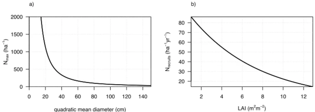
2.1.2 ORCHIDEE-CAN: self-thinning and recruitment scheme
In CAN, competition for light among trees is simulated through self-thinning. The maximum number of trees (Nmax) depends
on the mean stand diameter (Dg (m), Fig. 1a) as follows:
20
𝑁!"#= !!! !/!
(1)
with the parameters 𝛼 = 1100 (m) and 𝛽 = −0.57 estimated for tropical forests using publicly available plot-level data from the RAINFOR forest inventory network (Brienen et al., 2015).
25
In unmanaged tropical forests, the mortality of old trees takes place in parallel with the recruitment of young trees. To account for this natural plant regeneration, we implemented a recruitment scheme where the number of recruited trees (𝑁!"#!$%&' per hectare and per year, Fig. 1b) is a function of the LAI using the following equation:
30
5
This parameterization assumes that the number of recruits depends on mean-stand LAI. Note that in this version recruitment rate does not depend on the rate of canopy gap formation, in spite of the demonstrated importance of canopy openings for the regeneration of natural forests.
Figure 1. (a) self-thinning equation and (b) recruitment scheme for tropical forests in CAN
5
2.1.3 Implementing a dynamic root scheme
In CAN, the soil water potential in the rooting zone (𝛹!", MPa) is calculated as the weighted sum of the soil water potential
per layer (𝛹!, MPa), weighted by the relative proportion of root biomass in each layer 𝑑!""#. An additive tuning factor (𝑚!)
10
accounts for missing processes, such as the hydraulic resistance at the soil-root interface (Naudts et al., 2015) :
𝛹!"= !!!!𝛹! 𝑙 𝑑!""# 𝑙 + 𝑚! (3)
where L is the number of layers (L=12). 15
𝛹! is calculated for each soil layer l and depends on the layer volumetric water content (Θ l m3 m-3) following the Mualem
-van Genuchten model (-van Genuchten, 1980; Mualem, 1976):
𝛹! 𝑙 = min(!!!" !"# ! !!!!!!!! ! ! !!" − 1 ! !!" ; −5) (4) 20
where SWC(l) is soil water content in layer l; 𝛩! and 𝛩! (m3 m-3) are the residual and saturated SWC, respectively; and
𝑘!", 𝑘!" 𝑎𝑛𝑑 𝑘!" are the van Genuchten parameters. These parameters are texture-dependent (see Table S1). 𝛹! cannot be
0 20 40 60 80 100 120 140 0 500 1000 1500 2000
quadratic mean diameter (cm)
Nm a x (ha − 1) a) 2 4 6 8 10 12 20 30 40 50 60 70 80 LAI (m2m−2) Nre c ru it s (ha − 1yr − 1) b)
lower than the soil water potential for hygroscopic water (-5 MPa) (Larcher, 2003).
The use of root biomass-weighted sum of soil layer moisture in Eq. (3) ignores the dependence of soil-to-root water flow on soil and root hydraulic properties. Besides, the use of 𝑚! often leads to incorrect positive hydraulic potentials. We therefore
implemented a different computation of 𝛹!", whereby 𝛹! is weighted by 𝐸!"#(𝑙), the maximum amount of water (mmol m2
5
s-1) that can be absorbed by the roots in each layer, which itself depends on the soil-to-root resistance 𝑅
!" (MPa s mmol-1 m
-2) and on a minimum root water potential 𝛹
!""#,! (MPa) (Duursma and Medlyn, 2012; Fisher et al., 2006; Williams et al.,
2001). Replacing Eq. (3) by the following equation in CAN leads to the version hereafter called CAN-RS.
𝛹!"= !!! !!"# ! ! ! !!"# (!) ! ! with 𝐸!"# 𝑙 = [𝛹! 𝑙 − 𝛹!""#,!] 𝑅!"(𝑙) (5) 10
𝛹!""#,! is a parameter set at -3 MPa (Duursma and Medlyn, 2012). The soil-to-root resistance 𝑅!" estimates the effective
pathlength for water transport from the soil matrix to the root surface (Gardner, 1960), and is computed as follows: 𝑅!" 𝑙 =
!"!! !
!!
! ! !!! !!"#$! !!(!) (6)
Here, 𝑙! (m-2) is the root length per unit of soil volume, and is a function of the specific root length (SRL), with SRL set at 10
15
m g-1 (Metcalfe et al., 2008), and of the fine root biomass density per layer (𝐵𝑖𝑜𝑚𝑎𝑠𝑠
!"##$% 𝑙 , in g m-3):
𝑙! 𝑙 = 𝐵𝑖𝑜𝑚𝑎𝑠𝑠!"##$% 𝑙 𝑆𝑅𝐿; 𝑟! (m) is one-half of the mean distance between roots, computed following (Newman,
1969): 𝑟!= ! !! !(!) !.! (7) 20
and 𝑟! (m) is the mean fine root radius, set at 0.29 10-3 m (Bonan et al., 2014); 𝐺!"#$ (mmol m-1 s-1 MPa-1) is the saturated
hydraulic conductivity for the soil (see section 2.1.3). In CAN, 𝐵𝑖𝑜𝑚𝑎𝑠𝑠!"##$% is calculated following the allocation scheme
relying on the pipe model theory (Shinozaki, 1964; Sitch et al., 2003) and it is vertically discretized per soil layer by multiplying by 𝑑!""# 𝑙 .
25
2.1.3 Soil characteristics
In all three versions of ORCHIDEE considered in this study, the relationships between saturated hydraulic conductivity, volumetric water content, and matrix potential are described by the Mualem–van Genuchten model (van Genuchten, 1980; 30
7
Mualem, 1976), using the parameters estimated by Carsel and Parrish, [1988] for the 12 soil texture classes of the United States Department of Agriculture (USDA) classification.
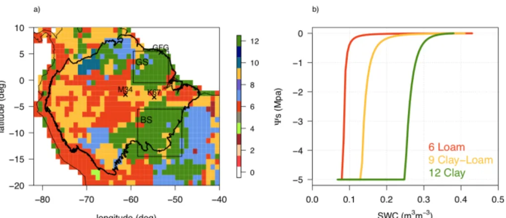
Figure 2. (a) USDA soil types interpolated at 1-degree resolution over the Amazon used as a forcing to ORCHIDEE, where GS and BS squares represent the Guianan and Brazilian Shields respectively; and (b) the soil water retention
5
curves (𝜳𝒔 versus SWC) predicted by the Mualem-van Genuchten equation (Eq. 4) for the three dominant USDA soil
classes in Amazonia. Parameter values are given in the SI (Table S1).
The spatial heterogeneity of soil structure in Amazonia is related to the geology of the area with old, highly weathered soils (Precambrian substrates) over the Brazilian and Guianan Shields contrasting with the much younger Cenozoic geology of the 10
Andes and western Amazonia (Quesada et al., 2011). This is reflected in the USDA map of soil types, with mainly clayey (12) soil type over the shields, and loam (6) and clay-loam (9) over the rest of Amazonia (Fig. 2a). The Mualem-van Genuchten equation (Eq. 4) implies lower water availability for plants in clayey soils than for those in loam or clay-loam soils, at a given soil water content (i.e., more negative values 𝛹! for the same SWC; Fig. 2b).
15
2.1.4 Simulations
To investigate the effect of both hydraulic processes and model structure on the simulated forest dynamics of Amazonia, we compared outputs from the TRUNK version as used in the Sixth Model Intercomparison Project (CMIP6), the CAN (v2290) version parameterized for tropical forests, and CAN-RS. All three versions were run using 13 plant functional types (PFTs) 20
and the multi-layer diffusion scheme [de Rosnay et al., 2002] considering a 4-metre soil depth and 12 soil layers (Campoy et al., 2013).
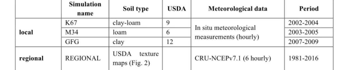
Firstly, simulations were performed at three sites across Brazil and French Guiana for which eddy-covariance measurements were available (da Rocha, 2004): Santarem KM67 (K67), Manaus KM34 (M34) (da Rocha et al., 2009) and Paracou (GFG) (Bonal et al., 2008). The evergreen tropical forest PFT cover was used. All simulations used hourly local meteorological 25
forcing. Each site corresponds to one of the major soil texture classes according to USDA soil classification (Fig. 2 and Table 1). Secondly, regional historical simulations were performed at 1-degree spatial resolution over the Amazonian forest using up-scaled gridded climate forcing data from CRUNCEP, which combine monthly data from the Climate Research Unit (CRU) and 6-hourly fields from the National Center for Environmental Prediction (NCEP) (Wei et al., 2014) (Table 1). All simulations started from a semi-analytical spin-up (Lardy et al., 2011) to equilibrate carbon and hydrological variables by 5
recycling climate data from 1981 to 2000 under a constant CO2 concentration set to 370 ppm.
Table 1. Summary of the simulations. All four simulations were run with the TRUNK, CAN and CAN-RS versions. Simulation
name Soil type USDA Meteorological data Period local K67 clay-loam 9 In situ meteorological measurements (hourly) 2002-2004 M34 loam 6 2003-2005 GFG clay 12 2007-2009
regional REGIONAL USDA texture
maps (Fig. 2) CRU-NCEPv7.1 (6 hourly) 1981-2016
2.2 Observations used as benchmarks
10
2.2.1 Site data
At all three tropical forests sites (Bonal et al., 2008; da Rocha et al., 2009), measurements include hourly turbulent sensible (H) and latent (LE) heat fluxes, and net ecosystem carbon exchange (NEE) made using the eddy-covariance technique 15
(Baldocchi et al., 2001; Shuttleworth et al., 1984). Gross primary productivity (GPP) and ecosystem respiration were retrieved from NEE using the algorithm of Reichstein et al., [2005]. Flux data are noisy, and Hollinger and Richardson, [2005] evaluated the relative uncertainty of H, LE and CO2 fluxes derived from eddy-covariance measurements to be around
25% for a temperate site. For eddy-covariance data, energy balance closure is a good proxy for data quality (Wilson, 2002). Wetherefore calculated the overall energy balance ratio as the ratio of the sum of outgoing radiation (LE + H) divided by the 20
sum of incoming radiation averaged over the study period (Wilson, 2002). K67 and GFG showed a consistent energy closure (ratio of 1.008 and 0.96 respectively), but at M34 energy fluxes should be interpreted carefully as energy closure was not achieved (ratio of 0.69).
Reported LAI, basal area (BA), and canopy height, (references in Table 2), were used to benchmark the site-level 25
simulations. At K67, a vertical soil moisture profile was available (Nepstad et al., 2007). At GFG, old-growth forest plots were surveyed (Gourlet-Fleury et al., 2004; Ho Tong Minh et al., 2016). We used tree diameter and height measurements (for 1592 trees) from the 2014 inventory on a 6.25 ha plot. Forest inventories used in this study only included trees measured
9
above a DBH of 10 cm. Data from a site near to GFG that had been clear-cut in 1976 and then left to regenerate were also used to evaluate forest regeneration in CAN and CAN-RS [Chave et al., in prep].
2.2.2 Regional datasets
To evaluate GPP patterns and seasonality at regional scale, we used the monthly global observation-based GPP model 5
FLUXCOM, running from 1981 to 2013 and produced at 0.5° resolution using different methods by Tramontana et al., [2016] and Jung et al., [2017]. We calculated the median of the following three methods, namely ANNs (artificial neural networks), RF (Random Forest) and MTE (Model Tree Ensemble) and chose the method proposed by Lasslop et al., [2010] to retrieve GPP by fitting a respiration model to nighttime NEE values. All methods were highly consistent (not shown). Compared to the global network of flux-tower measurements, performances were reasonable in terms of annual mean and 10
spatial pattern representation (R2 > 0.7) and mean seasonal cycle (0.67 < R2 < 0.77), but they showed a low predictive power
for interannual variability (Tramontana et al., 2016). Also, GPP (and other fluxes) were better predicted in temperate climate sites than in the tropics due to a smaller amount of training data being available (Tramontana et al., 2016).
For ET, we used the remotely sensed GLEAM v3.1a product [Martens et al., 2017 and references within] interpolated at 1-15
degree resolution from 1981 to 2016. To illustrate the uncertainties associated with this global dataset, GLEAMv3.1 was compared to the ET measurement at K67 (M34) between 2000 and 2006, Moreira et al., [2018] found a relatively strong bias of 0.77 (0.99) mm d-1 and low correlation -0.08 (0.32).
Furthermore, we used a compilation of 413 ground inventories across Amazonia presented by Mitchard et al., [2014]. Basal 20
area (BA) was directly calculated from diameter measurements, and aboveground biomass (AGB) was retrieved using the three-parameter moist tropical forest allometric model of Chave et al., [2005].
3. Results
25
3.1 Site-level evaluation of the models
While TRUNK has been evaluated over Amazonia (Getirana et al., 2014; Guimberteau et al., 2012, 2014), CAN has been evaluated for European forests only. All three model versions (TRUNK, CAN and CAN-RS) predicted the yearly mean state of forest features (such as LE, GPP, LAI) with a bias < 20% at the three test sites (Table 2). CAN and CAN-RS predicted 30
more productive forests with higher biomass (higher LE, GPP, AGB, LAI) than TRUNK. At M34, CAN and CAN-RS overestimated LE, but the energy budget was not closed at this site (see Methods). TRUNK simulated an AGB lower than the observed one, and CAN and CAN-RS generally overestimated AGB, especially at K67, where the overestimate by CAN and CAN-RS was 25% and 31%, respectively. This overestimation of AGB may possibly result from recent disturbances
[Pyle et al., 2008] that the models did not take into account. Finally, CAN and CAN-RS tended to underestimate tree height and overestimate basal area (Table 2).
Table 2. Comparison of TRUNK, CAN and CAN-RS against observations made at K67, M34 and GFG. Mean percentage bias between the observations and model results are highlighted in green when < 20%, in blue when between 20 to 40% and in red when > 40%.
5
VARIABLE
Site
OBS
TRUNK
CAN
CAN-RS
Refs and remarks
LE
(W m
-2)
K67
86
70
87
89
Eddy-covariance measurements (Bonal et al., 2008;
da Rocha et al., 2009)
M34
79
91
132
131
GFG
119
92
102
115
GPP
(µmol CO
2m
2s
-1)
K67
8.2
7.7
6.3
7.4
M34
7.9
7.5
8.1
8.1
GFG
9.7
7.6
7.8
9.6
AGB
(tC ha
-1)
K67
148 ± 3
101
198
214
(Pyle et al., 2008) recently disturbed plot
M34
180 ± 10
99
221
221
(Malhi et al., 2009b)
GFG
203
102
206
228
(Dubois-Fernandez et al., 2012)
LAI
(m
2m
-2)
K67
6.4 ± 0.1
4.9
6.2
6.6
(Malhi et al., 2009a)
M34
5.6 ± 0.2
4.8
6.7
6.7
(Malhi et al., 2009a) (hemiphoto method)
GFG
8.6 ± 0.7
5.0
6.5
7.3
[Granier et al., 1996] (Demon Leaf Area Method)
Canopy
Height
(m)
K67
29.1 ± 7.2
-
19
19.1
(Meyer et al., 2018) (Fig. S3) mean canopy height
model (CHM) at 1 m resolution from LIDAR and
associated standard deviation
M34
26.7 ± 6.8
-
19.5
19.6
GFG
29.7 ± 9.5
-
19.4
20.2
Basal Area
(m
2ha
-1)
K67
31
-
36.1
36.2
[Hunter et al., 2008]
M34
27
-
36.6
36.6
[Rodrigues et al., 2001]
GFG
31.6
-
36.5
37.3
[Ferry et al., 2006] (Table 4)
3.1.1 Seasonal water and carbon fluxes
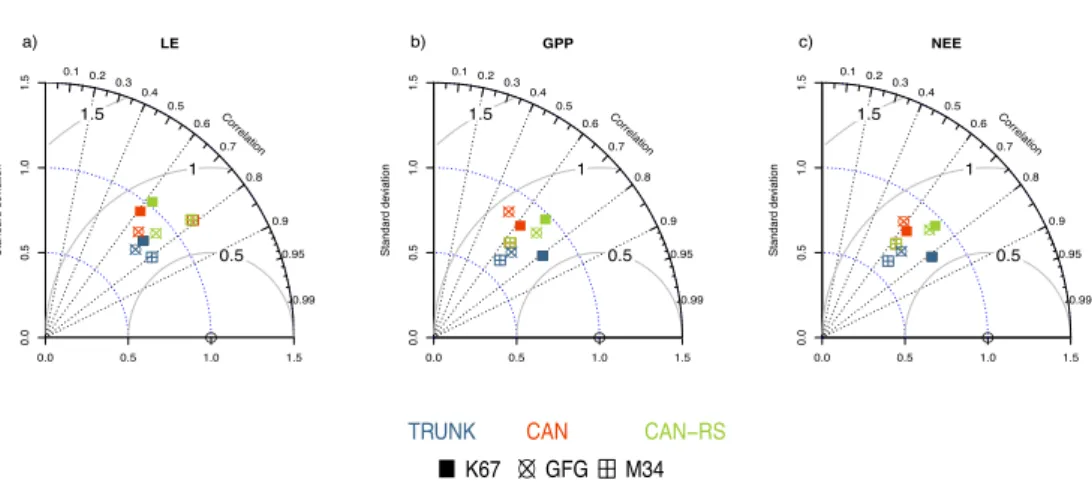
Looking at the time series of LE, GPP and NEE at the three sites, the three model versions displayed reasonable scores with temporal correlations between observations and simulations varying from 0.6 to 0.8; the normalized standard deviation and RMSE ranked from 0.5 to 1 (Fig. 3). CAN-RS represented the standard deviation better than TRUNK, but not the 10
correlation. CAN-RS outperformed CAN at two of the sites, K67 and GFG, but not at M34 where the two models had a similar performance (Fig. 3).
11
Figure 3. Taylor Diagrams (Taylor, 2001) for: (a) LE, (b) GPP and (c) NEE, at three Amazonian sites equipped with a eddy-flux tower systems. These quantities were calculated among hourly values removing nighttime values (defined by downwelling shortwave radiation ≤ 5 W m−2). In a Taylor diagram, correlation extends radially from the origin.
5
The blue concentric lines indicate identical ratios of standard deviation of the simulated flux to the observed flux. The grey lines represent identical root mean square errors (RMSE) of the centred fluxes.
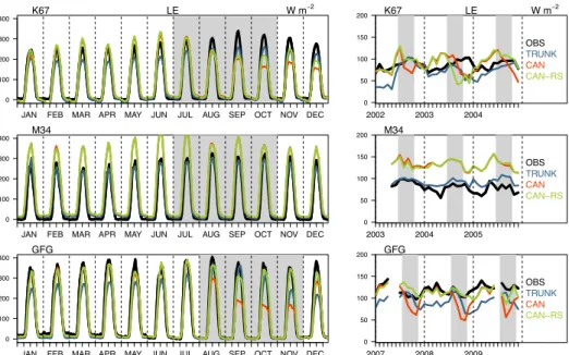
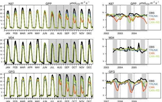
The effect of the soil-to-root resistance-weighting scheme on LE and GPP was strongly influenced by the soil type (Table 1 and Fig. 2). Little difference between CAN and CAN-RS was observed at site M34, because there, the soil is loamy, 10
implying a low water stress most of the year. At site GFG however, soil is clayey implying a high water stress during the dry season, and CAN-RS performed better than CAN, which underestimated LE and GPP by about 31% and 54%, respectively, during the dry season. At that site, TRUNK was also found to overestimate the seasonality of the fluxes. For site K67 with a clayey-loamy soil, implying an intermediate water stress, CAN-RS buffered the dry season drop in LE and GPP simulated by CAN during the first (2002) and third years (2004). In 2003, CAN-RS simulated a decrease in LE and GPP two months 15
sooner than CAN (Figs. 4 and 5).
CAN-RS better simulated the flux seasonality compared to CAN for soils prone to water stress during the dry season, by buffering the effect of drought stress. CAN-RS performance was comparable to TRUNK with, at daily time-steps, a better representation of the variability for all fluxes, but lower correlations for carbon fluxes (Fig. 3). CAN-RS simulated a midday 20
depression for GPP during dry seasons, which is not apparent in the data, resulting in a lower correlation between observations and simulations than for the TRUNK version (Fig. 4).
LE Standard de viation 0.0 0.5 1.0 1.5 0.0 0.5 1.0 1.5 0.5 1 1.5 ● 0.1 0.2 0.3 0.4 0.5 0.6 0.7 0.8 0.9 0.95 0.99 Correlation a) ● ● ● GPP Standard de viation 0.0 0.5 1.0 1.5 0.0 0.5 1.0 1.5 0.5 1 1.5 ● 0.1 0.2 0.3 0.4 0.5 0.6 0.7 0.8 0.9 0.95 0.99 Correlation b) ● ● ● NEE Standard de viation 0.0 0.5 1.0 1.5 0.0 0.5 1.0 1.5 0.5 1 1.5 ● 0.1 0.2 0.3 0.4 0.5 0.6 0.7 0.8 0.9 0.95 0.99 Correlation c) ● ● ● ● ● K67 GFG M34
Figure 4. Observed and simulated LE (W m-2) at the three sites. Left panels show the average diurnal cycle for each
month over three years; and right panels, monthly mean time series. Grey shaded areas indicate dry seasons (here defined as periods with precipitation less than 100 mm per month).
5 0 100 200 300 400 SA1OBSd[, x]
JAN FEB MAR APR MAY JUN JUL AUG SEP OCT NOV DEC
W m−2 LE K67 0 50 100 150 200 c(SA1OBSm[, x], rep(NA, 12)) 2002 2003 2004 W m−2 LE OBS TRUNK CAN CAN−RS K67 0 100 200 300 400 MA2OBSd[, x]
JAN FEB MAR APR MAY JUN JUL AUG SEP OCT NOV DEC
M34 0 50 100 150 200 c(MA2OBSm[, x], rep(NA, 12)) 2003 2004 2005 OBS TRUNK CAN CAN−RS M34 0 100 200 300 400 GFGOBSd[, x]
JAN FEB MAR APR MAY JUN JUL AUG SEP OCT NOV DEC
GFG 0 50 100 150 200 c(GFGOBSm[, x], rep(NA, 12)) 2007 2008 2009 OBS TRUNK CAN CAN−RS GFG
13
Figure 5. Observed and simulated GPP (µmolCO2 m-2 s-1) at the three sites. Left panels show the average composite
monthly diurnal cycle for each month over 3 years; and right panels, monthly mean time series. Grey shaded areas indicate dry seasons (here defined as periods with precipitation less than 100 mm per month).
5
3.1.2 Soil volumetric water content and transpiration
To better understand the effect of the new root water uptake scheme, we focus here on the K67 site, where direct observations of the variation of soil water content with depth are available. Deviations between observations and simulations may be due to using soil texture and van Genuchten parameters from the USDA soil parameterization — these might deviate 10
from actual soil at K67 (Figs. 6b-d). Besides, soil water content tended to be lower in CAN-RS than in CAN, especially during the dry seasons, in agreement with a higher LE simulated by CAN-RS (Fig. 4).
For the years 2002 and 2004, the soil-to-root resistance scheme implemented in the multilayer soil model allowed CAN-RS to overcome the too strong tree water stress simulated by CAN during dry seasons (Figs. 4 and 5) and 𝛹!" stayed close to
15
zero (Fig. 6e). Wet season rainfall restocked soil layers with water from top to bottom (Fig. 6d), and most layers then contributed to the transpiration flux (Fig. 6f). As the dry season progressed, the topsoil layers became drier due to stronger evaporation and harsher root competition, which induced a shift of water uptake towards deeper and wetter soil layers (Fig. 6f), where the soil-to-root resistance was lower (Eq. 6) and Emax higher (Eq. 7). Since the 2003 wet season was drier (1276
mm) than the ones in 2002 (1683 mm) and 2004 (1849 mm) (Fig. 6a), the amount of precipitation was insufficient to 20 0 5 10 15 20 25 30 SA1OBSd[, x]
JAN FEB MAR APR MAY JUN JUL AUG SEP OCT NOV DEC
µmolCO2 m−2 s−1 GPP K67 0 5 10 15 c(SA1OBSm[, x], rep(NA, 12)) 2002 2003 2004 µmolCO2 m−2 s−1 GPP OBS TRUNK CAN CAN−RS K67 0 5 10 15 20 25 30 MA2OBSd[, x]
JAN FEB MAR APR MAY JUN JUL AUG SEP OCT NOV DEC
M34 0 5 10 15 c(MA2OBSm[, x], rep(NA, 12)) 2003 2004 2005 OBS TRUNK CAN CAN−RS M34 0 5 10 15 20 25 30 GFGOBSd[, x]
JAN FEB MAR APR MAY JUN JUL AUG SEP OCT NOV DEC
GFG 0 5 10 15 c(GFGOBSm[, x], rep(NA, 12)) 2007 2008 2009 OBS TRUNK CAN CAN−RS GFG
recharge the soil after dry-season depletion (Fig. 6b-c). This translates into strong hydrological stress during the 2003 dry season, with daily 𝛹!" reaching -2.3 MPa (Fig. 6e). This failure to completely recharge the soil profile caused a significant
reduction in the simulated LE and GPP in 2003 (Figs. 4 and 5).
5
Figure 6. Daily times series from 2002 to 2004 at K67 of (a) precipitation, (b) observed soil moisture profile, (c) soil moisture (SWC) profile simulated in CAN (d) and soil moisture (SWC) profile simulated in CAN-RS, (e) soil water potential in the rooting zone (𝜳𝒓𝒛), and (f) simulated soil profile of the contribution of each layer to total root water
uptake Efrac(l) from CAN-RS, defined as Emax(l) divided by the sum of Emax across all layers.
15
3.1.3 Forest structure
We found that both CAN and CAN-RS both correctly reproduced forest establishment from bare soil based on empirical data on forest regeneration (Chave et al., in prep) in French Guiana near GFG (Fig. 7), starting with a fast increase in AGB and BA, which levelled off as self-thinning began.
5
Figure 7. Dynamics of (a) the aboveground biomass (AGB) and (b) basal area simulated by the different versions of ORCHIDEE soil during the first hundred years after clear-cut, compared to tree inventory data in the regeneration experiment ARBOCEL (REF) (Chave et al., in prep).
10
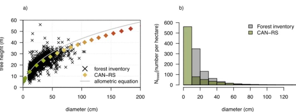
The representation of the forest by CAN-RS (or CAN), while more realistic than a big-leaf model (such as TRUNK), remains an approximation because it considers only 20 classes of tree diameter and mono-specific (single PFT) parameters within the forest. When comparing the simulated and measured forest structure at GFG using a forest inventory and measured tree heights (Fig. 8), CAN-RS and CAN showed a realistic diameter-height allometric relationship (Fig. 8a) and a diameter-size distribution with many small trees, and few large trees (Fig. 8b). However, the number of individuals was 15
slightly overestimated in CAN-RS with 800 trees ha-1 compared to 600 trees ha-1 from the forest inventory.
0 20 40 60 80 100 0 50 100 150 200 years A GB (tC ha − 1) REF TRUNK CAN CAN−RS a) 0 20 40 60 80 100 0 10 20 30 40 years BA (m 2ha − 1) REF CAN CAN−RS b)
Figure 8. Forest structure modelled in CAN-RS compared to forest inventory data over non-disturbed plots at Paracou (French Guiana), with (a) allometric relationship between tree diameter and tree height for the 20 simulated diameter classes in CAN-RS plotted in colours compared to 1592 measurements; plotted in grey, the diameter-height allometric equation for tropical forest proposed by Chave et al., [2014]; Eq. (6a); (b) mean diameter distribution per
5
hectare for CAN-RS compared to the 2014 forest inventory of a 6.25 ha plot in Paracou.
In CAN simulations we found more trees (930 trees ha-1), but with a smaller mean diameter (Fig. 9a). The higher GPP in
CAN-RS than in CAN (especially during the dry season; Fig. 4) allows CAN-RS to grow more large trees, (Fig. 9a), leading to a higher self-thinning effect, and slightly fewer saplings and poles than in CAN (Fig. 9b). This difference in forest 10
structure translates into a higher AGB than in CAN (228 versus 206 tC ha-1, Table 2).
Figure 9. Comparison between CAN-RS and CAN for: (a) mean trunk diameter per cohort, and (b) number of trees per cohort. Cohorts are illustrated as coloured bars numbered from 1 to 20, at Paracou, French Guiana (GFG).
15
3.2 Regional evaluation 3.2.1 Carbon and water fluxes
20 ● ● ● ● ● ● ● ●● ● ●● ● ● ● ● ● ● ● ● ● ● ●● ● ● ● ● ● ● ● ● ● ● ● ● ● ● ● ● ● ● ● ● ● ●● ● ● ● ● ● ● ● ● ● ● ● ● ● ● ● ● ● ● ● ● ● ● ● ● ● ● ● ● ● ● ● ● ● ● ● ● ● ● ● ● ●● ● ● ● ● ● ● ● ● ● ● ● ●● ● ● ● ● ● ● ● ● ● ● ● ● ● ● ●● ● ● ● ● ●● ● ● ● ● ● ● ● ● ● ● ● ● ● ● ● ● ● ● ● ● ● ● ●●● ● ● ● ● ● ● ● ● ● ● ● ● ● ● ● ● ● ● ● ● ● ● ● ●● ● ● ● ●●● ● ● ●● ● ● ● ● ● ● ● ● ● ● ● ● ●● ● ● ● ● ● ● ● ● ● ● ● ●● ● ● ● ● ● ● ● ● ● ● ● ● ● ● ● ● ● ● ● ● ● ● ● ● ●● ● ● ● ● ● ● ● ● ● ● ● ● ●● ● ● ●● ● ● ● ●● ● ●● ● ● ● ● ● ● ● ● ● ● ● ● ● ● ● ●● ● ● ● ● ●● ● ● ● ● ● ● ● ● ● ●● ● ● ●●●● ● ●● ● ● ● ● ●● ● ● ● ●●● ● ● ● ●● ● ● ● ● ● ● ● ● ● ● ● ● ● ● ● ● ● ● ● ● ● ● ● ●● ● ● ● ● ● ● ● ● ● ● ● ●● ● ● ● ● ● ● ● ● ● ● ● ● ● ● ● ● ● ● ● ● ● ● ● ● ● ● ● ●● ● ● ● ● ● ● ● ● ● ● ● ● ● ● ● ● ● ● ● ● ●● ● ● ● ● ● ● ● ● ● ● ● ● ● ● ● ● ● ● ● ● ● ● ● ● ● ● ● ● ● ● ●● ● ● ● ● ● ● ● ●● ● ● ● ● ● ● ● ● ● ● ● ● ● ● ● ● ● ● ● ●● ● ● ● ● ● ● ● ● ● ● ● ● ● ● ● ● ● ● ● ● ● ● ● ● ● ● ● ● ● ● ● ● ●● ● ● ● ● ● ● ● ● ● ● ● ● ● ● ● ● ● ● ● ● ● ● ● ● ● ● ● ● ● ● ● ● ● ● ● ● ● ● ● ● ● ● ●● ●● ● ● ● ● ● ● ● ● ● ● ● ● ● ● ● ● ● ● ● ● ● ● ● ● ● ● ● ● ● ● ● ● ● ● ● ● ● ● ● ● ● ● ● ● ● ● ● ● ● ● ● ● ● ● ● ● ● ● ● ● ● ●● ● ●● ● ● ● ● ● ● ● ●● ● ● ● ●● ● ●● ● ● ● ● ● ● ● ●● ● ● ●● ● ● ● ● ● ● ● ● ● ●● ● ● ● ● ● ● ● ● ● ● ● ● ● ● ● ● ● ● ● ● ●● ● ● ● ● ● ● ● ● ● ● ●● ● ● ● ● ● ● ● ● ● ● ● ● ● ● ● ● ● ● ● ● ● ● ● ● ● ● ● ● ● ● ● ● ● ● ● ● ● ● ● ● ● ● ● ● ● ● ● ● ● ● ● ● ● ● ● ● ● ● ● ● ● ● ● ● ● ● ● ● ● ● ● ● ● ● ● ● ● ● ● ● ● ● ●●● ● ● ● ● ● ● ● ● ● ● ●● ● ● ● ● ● ● ● ● ● ● ● ● ● ● ● ● ●● ●● ● ●● ● ● ● ● ● ● ● ● ● ● ● ● ● ● ●● ● ● ● ●● ●●●● ● ● ● ● ●●● ●● ● ● ●●● ● ● ● ● ● ● ● ● ● ● ● ● ● ● ● ● ● ● ● ● ● ● ●● ● ● ● ● ● ● ●● ● ● ● ●●●● ● ● ● ● ●●● ● ● ● ● ● ● ● ●● ● ● ●● ●● ● ●● ● ● ●● ● ● ● ● ● ● ● ●● ● ● ● ● ● ● ●● ● ● ● ●● ●● ●●●● ● ● ● ● ● ● ● ● ● ● ● ● ●● ●● ● ● ● ● ● ● ●● ● ● ● ● ● ●●●●● ●●●● ● ● ● ● ● ● ●●● ● ● ● ● ● ● ●●● ● ● ●● ●● ● ● ● ● ● ● ●● ● ●●● ● ● ●●● ● ● ● ● ● ● ● ● ●●●● ● ● ● ● ● ●● ● ● ● ● ● ● ● ● ● ● ● ● ● ●●●● ●● ● ● ● ● ● ● ● ● ● ● ● ● ● ● ● ● ● ●● ● ● ● ● ● ● ● ● ● ● ● ● ● ● ● ●● ● ● ●●● ● ● ● ● ● ●● ● ● ● ● ●●● ● ● ● ● ● ● ● ● ● ● ● ● ● ●● ● ● ●● ● ● ● ● ● ● ● ● ●● ● ● ● ● ● ● ● ● ● ● ● ● ● ● ● ● ●● ● ● ● ● ● ● ● ● ● ● ● ● ● ● ●● ● ● ● ●● ● ● ● ● ● ● ● ● ● ● ● ● ● ● ● ● ●● ● ● ●● ● ● ● ● ● ●● ● ● ● ● ● ● ● ● ●● ● ● ● ● ● ● ● ● ● ● ● ● ● ● ● ● ● ● ● ● ● ● ● ● ● ● ● ● ● ● ● ● ●● ● ● ● ●● ● ● ● ● ● ● ●● ● ● ● ● ● ● ● ● ● ● ● ● ● ● ● ●● ● ● ● ●● ● ●● ● ● ● ● ● ● ● ● ● ● ● ● ● ● ● ● ● ● ● ● ● ●● ●●● ● ● ● ● ● ● ● ● ● ● ● ● ● ● ● ● ● ● ● ● ● ● ● ● ● ● ● ● ● ● ● ● ● ● ● ●● ● ● ● ● ● ●●● ● ●● ● ● ● ● ● ● ● ● ● ● ● ● ● ● ● ● ● ● ●● ● ● ● ● ● ●● ● ● ● ● ● ● ● ● ● ● ●●● ● ● ● ● ● ● ●● ● ● ●● ● ● ● ● ● ● ● ●●● ● ● ● ● ● ● ● ● ● ● ● ● ● ●● ● ● ● ● ● ● ● ● ● ● ● ● ● ● ● ● ● ● ● ●●●●● ● ●●● ● ● ● ● ●● ● ● ● ●● ●● ● ● ● ● ●● ●● ● ● ● ●● ● ● ●●● ● ● ● ● ● ●● ● ● ● ● ●● ● ●● ● ● ● ● ● ● ● ● ● ● ● ●● ● ● ● ● ● ● ● ● ● ● ● ● ● ● ● ● ● ● ● ● ● ● ● ● ● ● ● ● ● ● ● ● ● ● ● ● ● ● ● ● ● ●● ● ●● ● ● ● ● ● ● 0 50 100 150 200 0 10 20 30 40 50 60 diameter (cm)
tree height (m) forest inventory CAN−RS allometric equation a) diameter (cm) Ntr e e s (n
umber per hectare)
0 100 200 300 400 500 600 0 20 40 60 80 100 120 Forest inventory CAN−RS b)
∆(CAN−RS − CAN) Diameter
∆ (cm) 0 5 10 15 20 25 a) 1 2 3 4 5 6 7 8 910 11 12 13 14 15 16 17 18 19 20
∆(CAN−RS − CAN) Individuals
∆ (Nb trees/ha) −40 −30 −20 −10 0 b) 1 2 3 4 5 6 7 8 9 10 11 12 13 14 15 16 17 18 19 20
17
Compared to the in situ fluxes at the three sites, both TRUNK and CAN-RS simulated ET and GPP reasonably well, except at M34 (Fig. 4 and Table 2). At regional scale, however, both models slightly overestimated annual LE (Fig. 10) and GPP (Fig. 11) when compared to the regional GLEAM LE and FLUXCOM GPP products. Differences can be partly explained by the fact that at local scale, models were forced with hourly local meteorological data, while for regional simulations we used the 6-hourly CRU-NCEP fields. Another explanation is the large uncertainties associated with the regional products over the 5
tropics. For example, both models correctly simulated total ET as compared with the ET product from Jung et al., [2011] covering the 1982-2008 period (Fig. S1).
ET and GPP simulated by CAN-RS reproduced the spatial pattern from GLEAM ET and FLUXCOM GPP, with higher annual fluxes in the northeast and southwest of Amazonia, and lower GPP along the southeast border (Figs. 10a;c, 11 a;c). In 10
CAN-RS these patterns were mainly driven by a relatively high downwelling shortwave radiation, and higher precipitation in these areas (Fig. S2). TRUNK simulated a more homogeneous pattern and was less sensitive to climate gradients than CAN-RS.
Figure 10. Annual mean (1982-2008) ET simulated by (b) TRUNK and (c) CAN-RS compared to the GLEAM
15
product (a).
Figure 11. Annual mean (1981-2013) GPP simulated by the TRUNK (b) and CAN-RS (c) compared to the FLUXCOM GPP product (a).
CAN-RS simulated higher annual mean ET and GPP than CAN over the Guianan and Brazilian Shields (Fig. 2, Fig. 12a, Fig. 13a). Comparison of monthly time series averages across the shields (Figs. 12a and 13a) shows that CAN-RS gives a better fit than CAN for both ET (0.81 versus 0.21 in the Guianan Shield, and 0.52 versus 0.40 in the Brazilian Shield) and GPP (0.42 versus 0.32 in the Guianan Shield, and 0.73 versus 0.67 in the Brazilian Shield). CAN simulated a drastic reduction in LE and GPP during the dry seasons (Fig. S3) and even in the months following, while CAN-RS simulated a 5
higher dry-season ET and GPP that better matched the dry-season observations (Figs. 12b and c, Figs. 13b and c) and simulated a more realistic SWC-GPP relationship (Fig. 14).
Figure 12. (a) Difference in predicted annual mean evapotranspiration (ET) between the
simulations of CAN-RS and CAN from 1982 to 2016. Comparison of the reference (GLEAM) and
10
simulated ET (TRUNK, CAN and CAN-RS) mean seasonal cycle over (b) the Guianan Shield, and
(c) the Brazilian Shield, including all pixels with at least 50% cover by evergreen tropical forest.
The envelopes represent the monthly minimum and maximum over the entire period for each
variable.
15
Figure 13. (a) Difference in predicted annual mean GPP between the simulations of CAN-RS and
CAN from 1981 to 2013. Comparison of the observed GPP and simulated GPP (TRUNK, CAN
and CAN-RS) mean seasonal cycle over (b) the Guianan Shield, and (c) the Brazilian Shield.
Envelopes describe the minimum and maximum values over the considered period, including all
20
19
Figure 14. Scatter plot of monthly GPP vs. monthly soil water content over (a) the Guiana Shield and (b) the Brazilian Shield simulated by CAN and CAN-RS from 1982 to 2016
3.2.2 Carbon stocks
5
The AGB stocks simulated by TRUNK were half of those simulated by CAN-RS (Figs. 15a and b), and CAN-RS also predicted a higher AGB than CAN over the Guianian and Brazilian Shields, due to higher GPP during the dry seasons (Fig. 13). This is explained by differences in parameterization and in the tree mortality processes, keeping in mind that only crowding mortality is modelled and not climate-induced (drought) mortality. In Amazonia, the simulated carbon-use 10
efficiency (CUE, the ratio of NPP to GPP) was higher in CAN-RS (0.42) than in TRUNK (0.30), because of lower maintenance respiration (RA,m) in CAN-RS (3.1 versus 5.3 gC m2 d-1) as the growth respiration was slightly higher (1.4
versus 1.1 gC m2 d-1). CAN-RS overestimated AGB, especially in the southwest part of the basin, but we emphasize that the
model was calibrated using sites with relatively high AGB mainly located in the northeast of Amazonia (Table 1, Fig. 2 and Fig. 16). Results from both models fit in the range of CUE field observations ranking from 0.27 to 0.52 (Malhi et al., 2009a, 15
2015), but in CAN-RS (and CAN), RA,m is calculated for each living compartment as a function of temperature, biomass,
prescribed carbon/nitrogen ratio and kcmaint,the fraction of allocatable photosynthates consumed for maintenance and growth
respiration (which is a tunable parameter, see Table S2). Parameter kcmaint is poorly constrained by observations (Sitch et al.,
2003), and it can be optimized (e.g., as by Naudts et al. (2015)) for each site) or manually tuned, as in this study. TRUNK simulated a lower CUE, but underestimated AGB (Table 1, Fig. 15). Contrary to CAN in which mortality is an emerging 20
result of modelled competition processes via self-thinning (Fig. 1), in TRUNK the background tree mortality is very simply set as a constant fraction of the woody carbon pool, defined by a “residence time” parameter which is poorly constrained by observations (Sitch et al., 2003). Thus, it is possible to capture a realistic AGB with TRUNK by adjusting this residence time value, while in CAN-RS and CAN tuning the model to reproduce AGB is not trivial. Nevertheless, the three model versions
● 0 500 1000 1500 2000 0 5 10 15 20 Guianan shield
Soil water content (kg m−3)
GPP (gC m 2d − 1) CAN CAN−RS a) ● 0 500 1000 1500 2000 0 5 10 15 20 Brazilian shield
Soil water content (kg m−3)
GPP (gC m 2d − 1) CAN CAN−RS b)
appear to lack the mechanisms underlying the observed SW-NE gradient in AGB, that have been hypothesized to relate to soil fertility (phosphorus), tree species or soil mechanical resistance.
Figure 15. Annual mean of aboveground biomass (AGB) from 2000 to 2010 simulated by (a) TRUNK and (b) CAN-RS. Panel (c) shows the difference between CAN-RS and CAN.
5
Figure 16. (a) fraction of evergreen tropical forests input in ORCHIDEE and location of the in situ inventories collected by Mitchard et al., [2014]; (b) comparison of simulated aboveground biomass and (c) basal area from the field inventory measurements along the SE-NW gradient indicated in (a).
10
4. Discussion
4.1 Root water uptake module and soil hydraulic parameters
15
With the mechanistic root water uptake module implemented in CAN-RS version of ORCHIDEE, trees preferentially used water in the deepest soil layer during the dry season. This reduced the effective decrease in leaf gas exchange induced by water stress. Through this process, the model better captured the seasonality of GPP and LE. The effect was strongest for soil types with a constraining soil water retention curve (e.g., clay USDA soil type 12). The root water uptake model was successfully validated under severe drought conditions (Fisher et al., 2006) and for other ecosystems (e.g. by Williams et al. 20
21
(Getirana et al., 2014; Guimberteau et al., 2014; Restrepo-Coupe et al., 2016), was unable to maintain LE and GPP fluxes during the dry season.
A previous modelling study using TRUNK showed the importance of deep roots by optimizing soil depth parameters at 10 m for seasonal variation of fluxes in Amazonia (Poulter et al., 2009; Verbeeck et al., 2011). However, this is a model artefact as 5
TRUNK’s water stress function directly links available soil moisture content to leaf gas exchange. Increasing soil depth in TRUNK will always increase the water storage capacity, but will not shift tree water uptake to the deepest layers during dry seasons since the root profile is fixed and exponentially decreases from top to bottom in the soil column. By using the soil-to-root resistance weighting scheme and a relatively deep soil (4 m) that contains most of the fine roots (as observed by Markewitz et al. (2010); Nepstad et al. (1994); Schenk and Jackson (2005)), CAN-RS sustains productivity by explicitly 10
simulating the observed shift of water uptake to deeper and wetter soil layers during the dry season (Moreira et al., 2000). Because of its explicit hydraulic architecture, CAN and CAN-RS are more sensitive than TRUNK (water stress function) to the parameters of the Mualem-van Genuchten Model (van Genuchten, 1980; Mualem, 1976). It is well known that changes in the spatial resolution of the soil input data by aggregating small-scale information causes serious problems in models (Van 15
Looy et al., 2017), as well as the use of co arse soil texture classes (Kishné et al., 2017). Thus, along with improving model representation of the hydraulic gradient from the soil to the plant in DGVMs [this study, Sperry et al., 2002; Fisher et
al., 2006], it is important to improve the parameterization of the physical soil environment (Marthews et al., 2014). While
increasing the spatial resolution is computationally expensive, accounting for variability of soil parameters rather than combining these parameters into texture classes (e.g., USDA texture class) may now be explored using, for example, 20
hydraulic parameters maps as developed by Marthews et al., [2014] at regional scale.
4.2 Missing processes to correctly capture spatial variability across Amazonia
As with most DGVMs (Castanho et al., 2015; Johnson et al., 2016), TRUNK, CAN and CAN-RS fail to capture the SW-NE 25
gradient of AGB (and BA) across Amazonia (Fig. 16) — they simulate a quasi-constant AGB across the basin (Fig. 15). This AGB gradient could be caused either by productivity or tree mortality. Spatial variation in wood productivity can be linked to spatial variability in soil properties [Quesada et al., 2012], like soil fertility [ter Steege et al., 2006 ; Malhi et al., 2004, Turner et al., 2018] and soil hydraulic parameters. Therefore, the incorporation of detailed soil hydraulic parameters maps (e.g., [Marthews et al., 2014]) and inclusion of nutrient cycles into ORCHIDEE would yield advances.
30
Besides variation in productivity, it has been shown that variation in tree mortality is a key driver of AGB across Amazonia [Johnson et al., 2016 and references within]. TRUNK, CAN and CAN-RS show a quasi-linear positive relationship between NPP and AGB, despite their differences in forest representation and tree mortality scheme over Amazonia (Fig. 18a) and
when focusing on different regions of the basin (Figs. S4 and S5). For high NPP, CAN-RS and CAN showed a saturation of GPP (not shown) and AGB around 250 tC ha-1 (Fig. 17a) due to a breakpoint in precipitation at 2000 mm yr-1 (Fig. 17b), this
phenomenon was also identified by Ahlström et al. [2017].
CAN-RS and CAN still lack functional diversity as a calibration of the self-thinning curve (Fig. 1), and all parameters 5
including wood density are constant within the “evergreen tropical forest” PFT covering most of Amazonia (Fig. 16a). Therefore, having a size distribution representation of the forest, as suggested by Johnson et al., [2016] is not sufficient, functional diversity needs to be accounted for in 2gDGVMs.
Figure 17. (a) scatter plots of mean AGB from 1981 to 2016 plotted against mean annual NPP and (b) annual
10
precipitation averaged over the same time period for Amazonia. 4.3. Concluding remarks
In this study, we demonstrated that a 2gDGVM (CAN-RS) can reproduce carbon and water fluxes and carbon stocks across 15
Amazonia, and we validated these simulations using local and regional observations. We also compared CAN-RS with earlier versions of the same family of models (ORCHIDEE-TRUNK and ORCHIDEE-CAN). The mechanistic root water uptake module implemented in CAN-RS allows trees to take up water in the deepest soil layer during dry seasons. This feature enables the model to capture the seasonality of GPP and LE, especially over the Guianan and Brazilian Shield (high water retention). The modelled diameter size distribution is improved compared to the TRUNK big-leaf DGVM. However 20
CAN-RS, by construction, still does not capture functional diversity, and behaves similarly to TRUNK. To include functional diversity in a 2gDVM, especially for tropical ecosystems, we believe that using soil hydraulic parameter maps (e.g., those from Marthews et al., [2014]) as an input is a necessary first step. Second, and because of the negative relationship between soil fertility and wood density (Baker et al., 2004; Patiño et al., 2009; ter Steege et al., 2006), and wood
● 0 10 20 30 40 50 0 50 100 150 200 250 300 NPP (tC ha yr−1) A GB tC ha − 1) TRUNK CAN CAN−RS ● 0 1000 2000 3000 4000 0 50 100 150 200 250 300 P (mm yr−1) A GB (tC ha − 1) TRUNK CAN CAN−RS
23
density and tree mortality (King et al., 2006); wood density should vary across the basin (rather than using a single parameter for the evergreen tropical forest PFT); this requires the use of wood density maps (ter Steege et al., 2006). Finally, mortality processes need to be linked to edaphic properties. Accounting for functional diversity in a 2gDGVM is crucial, not only to capture spatial patterns of Amazonian forest, but also to estimate its resilience to climate change (Sakschewski et al., 2016). 5
Aknowledgments
Data acquisition in French Guiana was supported by an “investissement d’avenir” grant from the Agence Nationale de la Recherche (CEBA, ref ANR-10-LABX-25-01). J.B. acknowledges support from (CR)2 Chile
(CONICYT/FONDAP/15110009). Matthieu Guimberteau, D. Goll and P. Ciais are funded by the European Research Council Synergy grant ERC-2013-SyG-610028 IMBALANCE-P. We also acknowledge the European Union Climate KIC 10
grant FOREST Specific Grant Agreement EIT/CLIMATE KIC/SGA2016/1CNES (TOSCA program) for funding.
References
Ahlström, A., Schurgers, G., Arneth, A. and Smith, B.: Robustness and uncertainty in terrestrial ecosystem carbon response to 15
CMIP5 climate change projections, Environ. Res. Lett., 7(4), 044008, doi:10.1088/1748-9326/7/4/044008, 2012.
Ahlström, A., Canadell, J. G., Schurgers, G., Wu, M., Berry, J. A., Guan, K. and Jackson, R. B.: Hydrologic resilience and Amazon productivity, Nat. Commun., 8(1), 1–9, doi:10.1038/s41467-017-00306-z, 2017.
Arora, V. K., Boer, G. J., Friedlingstein, P., Eby, M., Jones, C. D., Christian, J. R., Bonan, G., Bopp, L., Brovkin, V., Cadule, P., Hajima, T., Ilyina, T., Lindsay, K., Tjiputra, J. F. and Wu, T.: Carbon–Concentration and Carbon–Climate Feedbacks in 20
CMIP5 Earth System Models, J. Clim., 26(15), 5289–5314, doi:10.1175/JCLI-D-12-00494.1, 2013.
Baccini, A., Goetz, S. J., Walker, W. S., Laporte, N. T., Sun, M., Sulla-Menashe, D., Hackler, J., Beck, P. S. a., Dubayah, R., Friedl, M. a., Samanta, S. and Houghton, R. a.: Estimated carbon dioxide emissions from tropical deforestation improved by carbon-density maps, Nat. Clim. Chang., 2(3), 182–185, doi:10.1038/nclimate1354, 2012.
Baker, T., Phillips, O., Malhi, Y., Almeida, S., Arroyo, L., Di Fiore, A., Erwin, T., Higuchi, N., Killeen, T. J., Laurance, S. G., 25
Lewis, S. L., Monteagudo, A., Neill, D. a., Vargas, P. N., Pitman, N. C. a., Silva, J. N. M. and Martininez, R. V.: Increasing biomass in Amazonian forest plots, Philos. Trans. R. Soc. Lond. B. Biol. Sci., doi:10.1098/rstb.2003.1422, 2004.
Baldocchi, D., Falge, E. and Gu, L.: FLUXNET: A new tool to study the temporal and spatial variability of ecosystem-scale carbon dioxide, water vapor, and energy flux densities, Bull. Am. Meteorol. Soc., 82(11), 2415–2434, 2001.
Ball, J. T., Woodrow, I. E. and Berry, J. A.: A model predicting stomatal conductance and its contribution to the control of 30
photosynthesis under different environmental conditions, in Progress in Photosynthesis Research, pp. 221–224., 1987. Bellassen, V., Le Maire, G., Dhôte J.F., Ciais, P. and Viovy, N.: Modelling forest management within a global vegetation
model-Part 1: Model structure and general behaviour, Ecol. Modell., 221(20), 2458–2474, doi:10.1016/j.ecolmodel.2010.07.008, 2010.
Boisier, J. P., Ciais, P., Ducharne, A. and Guimberteau, M.: Projected strengthening of Amazonian dry season by constrained climate model simulations, Nat. Clim. Chang., (June), 1–6, doi:10.1038/nclimate2658, 2015.
Bonal, D., Bosc, A., Ponton, S., Goret, J.-Y., Burban, B., Gross, P., Bonnefond, J.-M., Elbers, J., Longdoz, B., Epron, D., Guehl, J.-M. and Granier, A.: Impact of severe dry season on net ecosystem exchange in the Neotropical rainforest of French Guiana, Glob. Chang. Biol., 14(8), 1917–1933, doi:10.1111/j.1365-2486.2008.01610.x, 2008.
5
Bonan, G. B., Williams, M., Fisher, R. A. and Oleson, K. W.: Modeling stomatal conductance in the earth system: linking leaf water-use efficiency and water transport along the soil–plant–atmosphere continuum, Geosci. Model Dev., 7(5), 2193–2222, doi:10.5194/gmd-7-2193-2014, 2014.
Booth, B. B. B., Jones, C. D., Collins, M., Totterdell, I. J., Cox, P. M., Sitch, S., Huntingford, C., Betts, R. A, Harris, G. R. and Lloyd, J.: High sensitivity of future global warming to land carbon cycle processes, Environ. Res. Lett., 7(2), 024002, 10
doi:10.1088/1748-9326/7/2/024002, 2012.
Brienen, R. J. W., Phillips, O. L., Feldpausch, T. R., Et Al., Gloor, E., Baker, T. R., Lloyd, J., Lopez-Gonzalez, G., Monteagudo-Mendoza, a., Malhi, Y., Lewis, S. L., Vásquez Martinez, R., Alexiades, M., Álvarez Dávila, E., Alvarez-Loayza, P., Andrade, a., Aragão, L. E. O. C., Araujo-Murakami, a., Arets, E. J. M. M., Arroyo, L., Aymard C., G. a., Bánki, O. S., Baraloto, C., Barroso, J., Bonal, D., Boot, R. G. a., Camargo, J. L. C., Castilho, C. V., Chama, V., Chao, K. J., Chave, 15
J., Comiskey, J. a., Cornejo Valverde, F., da Costa, L., de Oliveira, E. a., Di Fiore, a., Erwin, T. L., Fauset, S., Forsthofer, M., Galbraith, D. R., Grahame, E. S., Groot, N., Hérault, B., Higuchi, N., Honorio Coronado, E. N., Keeling, H., Killeen, T. J., Laurance, W. F., Laurance, S., Licona, J., Magnussen, W. E., Marimon, B. S., Marimon-Junior, B. H., Mendoza, C., Neill, D. a., Nogueira, E. M., Núñez, P., Pallqui Camacho, N. C., Parada, a., Pardo-Molina, G., Peacock, J., Peña-Claros, M., Pickavance, G. C., Pitman, N. C. a., Poorter, L., Prieto, a., Quesada, C. a., Ramírez, F., Ramírez-Angulo, H., Restrepo, 20
Z., Roopsind, a., Rudas, a., Salomão, R. P., Schwarz, M., Silva, N., Silva-Espejo, J. E., Silveira, M., Stropp, J., Talbot, J., ter Steege, H., Teran-Aguilar, J., Terborgh, J., Thomas-Caesar, R., Toledo, M., Torello-Raventos, M., Umetsu, R. K., van der Heijden, G. M. F., van der Hout, P., Guimarães Vieira, I. C., Vieira, S. a., Vilanova, E., Vos, V. a. and Zagt, R. J.: Long-term decline of the Amazon carbon sink, Nature, 519(7543), 344–348, doi:10.1038/nature14283, 2015.
Campoy, A., Ducharne, A., Cheruy, F., Hourdin, F., Polcher, J. and Dupont, J. C.: Response of land surface fluxes and 25
precipitation to different soil bottom hydrological conditions in a general circulation model, J. Geophys. Res. Atmos., 118(19), 10725–10739, doi:10.1002/jgrd.50627, 2013.
Carsel, R. F. and Parrish, R. S.: Developing joint probability distributions of soil water retention characteristics, Water Resour. Res., 24(5), 755–769, doi:10.1029/WR024i005p00755, 1988.
Castanho, A. D. A., Galbraith, D., Zhang, K., Coe, M. T., Costa, M. H. and Moorcroft, P.: Changing Amazon biomass and the 30
role of atmospheric CO2 concentration, climate, and land use, Global Biogeochem. Cycles, 30, 18–39,
doi:10.1002/2015GB005135.Received, 2015.
Chave, J., Andalo, C., Brown, S., Cairns, M. a, Chambers, J. Q., Eamus, D., Fölster, H., Fromard, F., Higuchi, N., Kira, T., Lescure, J.-P., Nelson, B. W., Ogawa, H., Puig, H., Riéra, B. and Yamakura, T.: Tree allometry and improved estimation of
25
carbon stocks and balance in tropical forests., Oecologia, 145(1), 87–99, doi:10.1007/s00442-005-0100-x, 2005.
Chave, J., Réjou-Méchain, M., Búrquez, A., Chidumayo, E., Colgan, M. S., Delitti, W. B. C., Duque, A., Eid, T., Fearnside, P. M., Goodman, R. C., Henry, M., Martínez-Yrízar, A., Mugasha, W. A., Muller-Landau, H. C., Mencuccini, M., Nelson, B. W., Ngomanda, A., Nogueira, E. M., Ortiz-Malavassi, E., Pélissier, R., Ploton, P., Ryan, C. M., Saldarriaga, J. G. and Vieilledent, G.: Improved allometric models to estimate the aboveground biomass of tropical trees, Global Change Biol., 5
20(10), 3177–3190, doi:10.1111/gcb.12629, 2014.
Christoffersen, B. O., Restrepo-Coupe, N., Arain, M. A., Baker, I. T., Cestaro, B. P., Ciais, P., Fisher, J. B., Galbraith, D., Guan, X., Gulden, L., van den Hurk, B., Ichii, K., Imbuzeiro, H., Jain, A., Levine, N., Miguez-Macho, G., Poulter, B., Roberti, D. R., Sakaguchi, K., Sahoo, A., Schaefer, K., Shi, M., Verbeeck, H., Yang, Z.-L., Araújo, A. C., Kruijt, B., Manzi, A. O., da Rocha, H. R., von Randow, C., Muza, M. N., Borak, J., Costa, M. H., Gonçalves de Gonçalves, L. G., Zeng, X. and 10
Saleska, S. R.: Mechanisms of water supply and vegetation demand govern the seasonality and magnitude of evapotranspiration in Amazonia and Cerrado, Agric. For. Meteorol., 191(February), 33–50, doi:10.1016/j.agrformet.2014.02.008, 2014.
Cox, P. M., Betts, R. A., Collins, M., Harris, P. P., Huntingford, C. and Jones, C. D.: Amazonian forest dieback under climate-carbon cycle projections for the 21st century, Theor. Appl. Climatol., 78(1–3), 157–175, doi:10.1007/s00704-004-0050-y, 15
2004.
Cox, P. M., Pearson, D., Booth, B. B., Friedlingstein, P., Huntingford, C., Jones, C. D. and Luke, C. M.: Sensitivity of tropical carbon to climate change constrained by carbon dioxide variability., Nature, 494(7437), 341–4, doi:10.1038/nature11882, 2013.
Deleuze, C., Pain, O., Dhote, J. and Hervé, J.-C.: A flexible radial increment model for individual trees in pure age stands, 20
Ann. For. Sci., 61(4), 327–335, doi:10.1051/forest, 2004.
Dubois-Fernandez, P. C., Le Toan, T., Daniel, S., Oriot, H., Chave, J., Blanc, L., Villard, L., Davidson, M. W. J. and Petit, M.: The tropiSAR airborne campaign in French Guiana: Objectives, description, and observed temporal behavior of the backscatter signal, IEEE Trans. Geosci. Remote Sens., 50(8), 3228–3241, doi:10.1109/TGRS.2011.2180728, 2012. Duursma, R. A. and Medlyn, B. E.: MAESPA: A model to study interactions between water limitation, environmental drivers 25
and vegetation function at tree and stand levels, with an example application to [CO2] and drought interactions, Geosci.
Model Dev., 5(4), 919–940, doi:10.5194/gmd-5-919-2012, 2012.
Eltahir, E. a. B. and Bras, R. L.: Precipitation recycling in the Amazon basin, Q. J. R. Meteorol. Soc., 120(518), 861–880, doi:10.1002/qj.49712051806, 1994.
Farquhar, G., Caemmerer, S. von and Berry, J.: A biochemical model of photosynthetic CO2 assimilation in leaves of C3
30
species, Planta, 90, 78–90, 1980.
Fischer, R., Bohn, F., Dantas de Paula, M., Dislich, C., Groeneveld, J., Gutiérrez, A. G., Kazmierczak, M., Knapp, N., Lehmann, S., Paulick, S., Pütz, S., Rödig, E., Taubert, F., Köhler, P. and Huth, A.: Lessons learned from applying a forest gap model to understand ecosystem and carbon dynamics of complex tropical forests, Ecol. Modell., 326, 124–133,