Data-Rich Multivariate Detection and Diagnosis
Using Eigenspace Analysis
by
Kuang Han Chen
B. Eng., McGill University, Montreal Canada, 1992 S. M., Massachusetts Institute of Technology, 1995
Submitted to the Department of Aeronautics and Astronautics
in partial fulfillment of the requirements for the degree of Doctor of Philosophy
at the
MASSACHUSETTS INSTITUTE OF TECHNOLOGY
June 2001
Massachusetts Institute of Technology, 2001. All Rights Reserved.Author ...
Department of Aeronautics and Astronautics May 18, 2001
Certified by ...
Professor Duane S. Boning Associate Professor of Electrical Engineering and Computer Science
Certified by ...
Professor Roy E. Welsch Professor of Statistics and Management
Certified by ...
Professor Eric M. Feron Associate Professor of Aeronautics and Astronautics
Certified by ...
Professor John J. Deyst Professor of Aeronautics and Astronautics
Accepted by ...
Professor Wallace E. Vander Velde Chairman, Department Committee on Graduate Students
Data-Rich Multivariate Detection and Diagnosis
Using Eigenspace Analysis
by
Kuang Han Chen
Submitted to the Department of Aeronautics and Astronautics on May 18, 2001, in partial fulfillment of the requirements for the
degree of Doctor of Philosophy in Aeronautics and Astronautics
Abstract
With the rapid growth of data-acquisition technology and computing resources, a plethora of data can now be collected at high frequency. Because a large number of char-acteristics or variables are collected, interdependency among variables is expected and hence the variables are correlated. As a result, multivariate statistical process control is receiving increased attention. This thesis addresses multivariate quality control techniques that are capable of detecting covariance structure change as well as providing information about the real nature of the change occurring in the process. Eigenspace analysis is espe-cially advantageous in data rich manufacturing processes because of its capability of reducing the data dimension.
The eigenspace and Cholesky matrices are decompositions of the sample covari-ance matrix obtained from multiple samples. Detection strategies using the eigenspace and Cholesky matrices compute second order statistics and use this information to detect sub-tle changes in the process. Probability distributions of these matrices are discussed. In par-ticular, the precise distribution of the Cholesky matrix is derived using Bartlett’s decomposition result for a Wishart distribution matrix. Asymptotic properties regarding the distribution of these matrices are studied in the context of consistency of an estimator. The eigenfactor, a column vector of the eigenspace matrix, can then be treated as a random vector and confidence intervals can be established from the given distribution.
In data rich environments, when high correlation exists among measurements, dominant eigenfactors start emerging from the data. Therefore, a process monitoring strat-egy using only the dominant eigenfactors is desirable and practical. The applications of eigenfactor analysis in semiconductor manufacturing and the automotive industry are demonstrated.
Thesis Supervisor: Duane S. Boning
Title: Associate Professor of Electrical Engineering and Computer Science Thesis Supervisor: Roy E. Welsch
Acknowledgments
It is a nice feeling to be able to write acknowledgments, remembering all the peo-ple that have been part of this long journey and have touched my life in so many ways. It has been a wonderful experience; I will cherish it for years to come.
I want to thank my advisor, Professor Duane Boning, for giving me the opportu-nity to work with him when I was at a cross road in my career. His support, insight and faith in me were the keys to the success of this work. He never ceases to amaze me with his ability to keep things in perspective and his wealth of knowledge in several areas.
I would like to thank my co-advisor, Professor Roy Welsch, from whom I have learnt so much in the field of applied statistics. His feedback and constructive criticism have taught me not to settle for anything less than what is best. Working as a TA by his side has allowed me to appreciate that teaching is a two-way action: to teach and to be taught.
I am grateful to Professor Eric Feron and Professor John Deyst for serving on my committee and taking time to read my thesis.
The support of several friends at MTL has made the process an enjoyable experi-ence. I will always remember the many stimulating conversations, either research related or just related to everyday life, I had with Aaron. I would also like to thank him for keep-ing the computers in the office runnkeep-ing smoothly durkeep-ing my thesis writkeep-ing. I am also thankful to Dave and Brian Goodlin for several great discussions on endpoint detection, Taber for showing me the meaning of “productivity” and the art of managing time to get 48 hours a day, and my extra-curricular activity companions Sandeep, Stuckey, Minh and Angie. Thanks also to our younger office mates Joe, Allan, Mike and Karen (who is already thinking of taking over my cubicle) for making our office more lively with their enthusiasm, Brian Lee, Tamba and Tae for their support, and in particular, Vikas for keep-ing me under control durkeep-ing my defense.
Throughout my graduate studies, my closest friends Joey and Yu-Huai have pro-vided me a shelter away from my worries. Their friendship and companionship have allowed me to take breaks and recharge myself as needed. I am grateful to all my MIT softball teammates for sharing the championships and glory over the past two years in the Greater Boston area and New England tournaments, especially to my friend Ken for being my sports-buddy for so many years.
My deepest thanks to Maria for being a source of both mental and emotional sup-port during the toughest time in my graduate work. Her belief in me has propelled me to derive the results and complete my thesis. I could not have done without her patience and encouragement, which have been vital during my thesis writing and defense.
I would like to thank my parents whose constant support and understanding have paved the way for me to get where I stand today. They have opened my eyes by providing me with the opportunity to experience different cultures and to adapt to new environments. A special thanks to my brother and sisters for putting up with me and for always sharing with me all the wonderful experiences that life offers.
Finally, I would like to thank the financial support of LFM/SIMA Remote Diag-nostic Program, LFM Variation Reduction Research Program and LFM GM Dimensional
Table of Contents
Chapter 1. Introduction ...13
1.1 Problem Statement and Motivation . . . .13
1.2 Thesis Outline . . . .14
Chapter 2. Background Information on Multivariate Analysis ...17
2.1 Control Chart and its Statistical Basis . . . .18
2.2 Multivariate Quality Control:χ2 and Hotelling’s T2 statistic . . . .20
2.2.1 Examples of Univariate Control Limits and Multivariate Control Limits . . . .22
2.3 Aspects of Multivariate Data . . . .26
2.4 Principal Components Analysis . . . .27
2.4.1 Data Reduction and Information Extraction . . . .29
2.5 SPC with Principal Components Analysis . . . .31
2.6 Linear Regression Analysis Tools . . . .34
2.6.1 Linear Least Squares Regression . . . .35
2.6.2 Principal Components Regression . . . .36
2.6.3 Partial Least Squares . . . .37
2.6.4 Ridge Regression . . . .38
Chapter 3. Second Order Statistical Detection: An Eigenspace Method ...41
3.1 Introduction . . . .41
3.2 First Order Statistical and Second Order Statistical Detection Methods . . . .42
3.2.1 First Order Statistical Detection Methods . . . .42
3.2.2 Second Order Statistical Detection Methods . . . .44
3.3 Weaknesses and Strengths in Different Detection Methods . . . .45
3.3.1 Univariate SPC . . . .45
3.3.2 Multivariate SPC First Order Detection Methods (T2) . . . .46
3.3.3 PCA and T2 methods . . . .47
3.3.4 Generalized Covariance . . . .49
3.4 Motivation Behind Second Order Statistical Detection Methods . . . .50
3.4.1 Example 1 . . . .51
3.4.2 Example 2 . . . .53
3.5 Eigenspace Detection Method . . . .56
3.5.1 Distribution of Eigenspace Matrix E . . . .60 3.5.2 Asymptotic Properties on Distribution of the Eigenspace Matrix E
and the Cholesky Decomposition Matrix M . . . .67
Chapter 4. Monte Carlo Simulation of Eigenspace and Cholesky Detection Strategy ...79
4.1 Introduction . . . .79
4.2 Simulated Distributions of Eigenspace Matrix and Cholesky Decomposition Matrix . . . .82
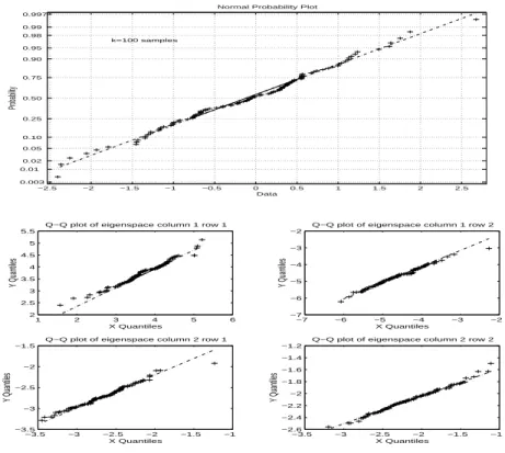
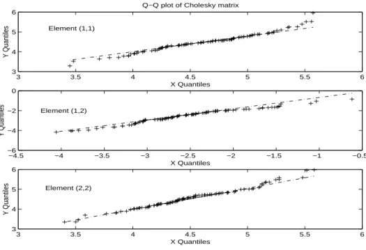
4.2.1 Example 1: N=20,000, n=50 and k=100 times . . . .84
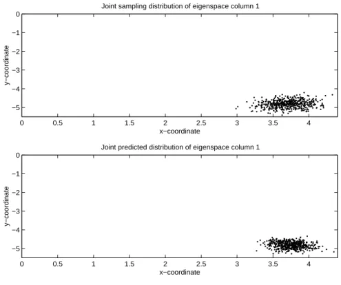
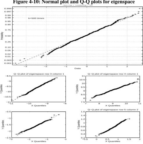
4.2.2 Example 2: N=20,000, n=500 and k=500 times . . . .88
4.2.3 Example 3: N=20,000, n=500 and k=500 times (8-variate) . . . .94
4.3 Approximation of Distribution of E and M for Large n . . . .99
4.3.1 Example 1: p=2, n=3, k=100 times 4.3.2 Example 2: p=2, n=100, k=100 times . . . .100
4.3.3 Example 3: p=10, n=500, k=500 times . . . .102
4.4 Sensitivity Issues: Estimation of Dominant Eigenfactors for Large p . . . . .105
4.4.1 Example 1: . . . .106
4.4.2 Example 2: . . . .110
4.5 Oracle Data Simulation . . . .112
4.5.1 Example 1: . . . .113
4.5.2 Example 2: . . . .118
Chapter 5. Application of Eigenspace Analysis ...125
5.1 Eigenspace Analysis on Optical Emission Spectra (OES) . . . .125
5.1.1 Optical Emission Spectra Experiment Setup . . . .126
5.1.2 Endpoint Detection . . . .128
5.1.3 Motivation for Application of Eigenspace Analysis to Low Open Area OES . . . .129
5.1.4 Low Open Area OES Endpoint Detection Results . . . .131
5.1.5 Control Limit Establishment for the Eigenspace Detection Method . . . .138
5.2 Eigenspace Analysis on Automotive Body-In-White Data . . . .142
5.2.1 Vision-system Measurements . . . .143
5.2.2 Out of Control Detection Using PCA and T2 Technique on the Left Door Data . . . .145
5.2.3 Eigenspace Analysis . . . .148
Chapter 6. Conclusions and Future Work ...153
6.1 Summary . . . .153
List of Figures
Chapter 1. Chapter 2.
Figure 2-1: A typical control chart . . . .19
Figure 2-2: Multivariate statistical analysis vs. univariate statistical analysis. . . . .22
Figure 2-3: Control limits for multivariate and univariate methods . . . .24
Figure 2-4: Graphical interpretation of PCA . . . .31
Figure 2-5: Graphical interpretation of T2 and Q statistics . . . .33
Chapter 3. Figure 3-1: T2 statistic drawback . . . .47
Figure 3-2: Drawback of T2 and T2 with PCA . . . .49
Figure 3-3: Two different covariance matrices in 2-D . . . .50
Figure 3-4: T2 values for example 1 . . . .52
Figure 3-5: A second order static detection method . . . .53
Figure 3-6: Generalized variance for example 2 . . . .54
Figure 3-7: A second order statical detection method . . . .55
Figure 3-8: Possibilities of two different population in 2-D . . . .56
Figure 3-9: Selection procedure of a unique eigenvector . . . .60
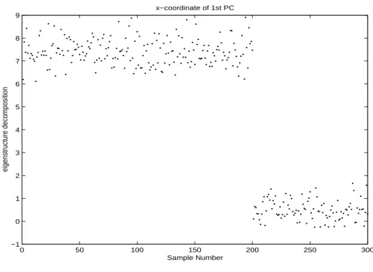
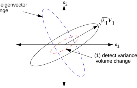
Chapter 4. Figure 4-1: Eigenfactor used to detect variance volume and eigenvector angle change . . . .81
Figure 4-2: Normal quantile plot for 100 samples and Q-Q plot for eigenfactor elements . . . .85
Figure 4-3: Q-Q plot for Cholesky decomposition matrix M . . . .86
Figure 4-4: Joint Distributions of eigenfactor 1 in E . . . .87
Figure 4-6: Normal plot and Q-Q plots for eigenfactor elements . . . .89
Figure 4-7: Q-Q plot for Cholesky Decomposition Matrix M . . . .90
Figure 4-8: Joint distribution of eigenfactor 1 . . . .91
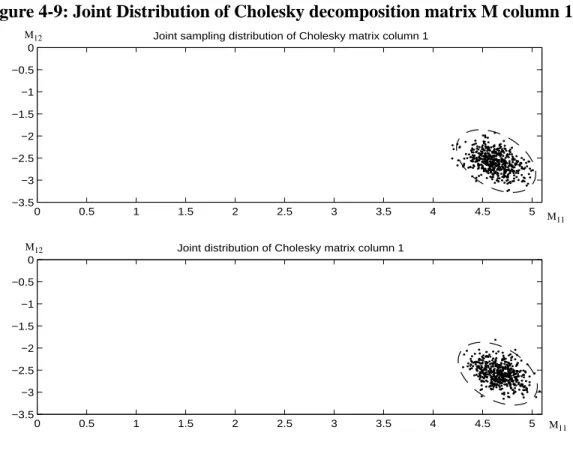
Figure 4-9: Joint Distribution of Cholesky decomposition matrix M column 1 . . . .92
Figure 4-10: Normal plot and Q-Q plots for eigenspace . . . .95
Figure 4-11: Q-Q plot for Cholesky Decomposition Matrix M . . . .96
Figure 4-12: Normal Q-Q plot of predicted and sampling distribution of E and M . . . .98
Figure 4-13: Normal Quantile plot for tii . . . .100
Figure 4-14: Normal Quantile plot . . . .102
Figure 4-15: Normal Quantile Plot of tii (high dimension) . . . .103
Figure 4-16: Normalization of d and total standard deviation . . . .108
Figure 4-17: Normalized 2-norm and total standard deviation as function of p . . . .109
Figure 4-18: Confidence interval for individual eigenfactor . . . .113
Figure 4-19: The T2 statistic detection . . . .114
Figure 4-20: Generalized variance detection using 100 samples window . . . . .115
Figure 4-21: Eigenspace detection . . . .116
Figure 4-22: Cholesky detection . . . .117
Figure 4-23: PCA with T2 and Q plots . . . .119
Figure 4-24: Generalized variance with 100-sample window . . . .120
Figure 4-25: Eigenspace detection using two columns with 100-sample window . . . .121
Figure 4-26: Cholesky detection using the first column with 100-sample window . . . .121
Chapter 5. Figure 5-1: Optical emission spectroscopy experiment setup . . . .126 Figure 5-2: Time evolution of spectral lines in an oxide
Figure 5-3: Two spectral lines showing different behavior as
endpoint is reached. . . .128
Figure 5-4: Plasma etch endpoint is reached when the intended etch layer (oxide) is completed removed . . . .129
Figure 5-5: Euclidean distance of (E1-Eep1) in run 4 . . . .132
Figure 5-6: Euclidean distance of (E1-Eep1) in run 5 . . . .133
Figure 5-7: Euclidean norm using characterization data from within the run (run 3) . . . .134
Figure 5-8: Euclidean norm of run 3 using characterization data from run 2 . . . .134
Figure 5-9: Euclidean norm of run 4 using characterization data from run 2 . . . .135
Figure 5-10: Euclidean norm of run 5 using characterization data from run 2 . . . .136
Figure 5-11: Euclidean distance for n=30 samples run 2 . . . .137
Figure 5-12: Euclidean distance for n=30 samples for run 4 . . . .138
Figure 5-13: Univariate control limits on multivariate normal data, applied to a selected eigenfactor . . . .139
Figure 5-14: Euclidean norm of run 5 with control limit . . . .141
Figure 5-15: Euclidean norm of run 5 using an overlapping sliding window of 50 samples . . . .142
Figure 5-16: Possible vision-system measurements on a door . . . .144
Figure 5-17: Scree Plot for the left door data . . . .145
Figure 5-18: The T2 plot for the left door data . . . .146
Figure 5-19: Scores and loading plots of record 50 (an out of control sample) . . . .147
Figure 5-20: Plot of standardized variable 20 across records . . . .148
Figure 5-21: The 2-norm of the difference between the sampling and population eigenfactor 1 . . . .149
Figure 5-22: Individual contribution across variables . . . .150
Chapter 6.
List of Tables
Chapter 1. Chapter 2. Chapter 3. Chapter 4.
Table 4-1: Properties of tii from simulated distribution . . . .104
Table 4-2: Mean and variance from example 3 (p=10 and n=500) . . . .104
Table 4-3: Summary of statistics as function of p for eigenfactor 1 . . . .106
Table 4-4: Summary of statistics as function of p for eigenfactor 2 . . . .107
Table 4-5: Summary of statistics as function of p for eigenfactor 1 . . . .110
Table 4-6: Summary of statistics as function of p for eigenfactor 2 . . . .110
Chapter 5. Chapter 6.
Chapter 1
Introduction
1.1 Problem Statement and Motivation
In large and complex manufacturing systems, statistical methods are used to monitor whether the processes remain in control. This thesis reviews and discusses both conven-tional methods and new approaches that can be used to monitor manufacturing processes for the purpose of fault detection and diagnosis. On-line statistical process control (SPC) is the primary tool traditionally used to improve process performance and reduce variation on key parameters. With faster sensors and computers, massive amounts of real-time equipment signals and process variables can be collected at high frequency. Due to the large number of process variables collected, these variables are often correlated. Conse-quently, multivariate statistical methods which provide simultaneous scrutiny of several variables are needed for monitoring and diagnosis purposes in modern manufacturing sys-tems. Thus, multivariate statistical techniques have received increased attention in recent research. Furthermore, data reduction strategies such as projection methods are needed to reduce the dimensionality of the process variables in data rich environments.
SPC has strong ties with input-output modeling approaches such as response surface methods (RSM). In order to build models for prediction, it is important to make sure that all the experiment runs are under statistical process control. Once one is confident in the prediction model, deviation of production measurement from the prediction could indicate process drift or other disturbances. In the case of process drift, adaptive modeling could be
used to include effects introduced by slowly varying processes. The purpose of RSM is to identify the source of product quality variation, in other words, to discover which in-line data contributes to end-of-line data variation. One can use experimental design approaches with projection methods to build statistical models between in-line data and end-of-line data. Both partial least squares (PLS) and principal components regression (PCR) are parametric regression techniques, and assume there is only one functional form to charac-terize the whole system; thus PLS and PCA can be labeled as “global modeling methods.” These global modeling methods impose strong model assumptions that restrict the poten-tial complexity of the fitted models, thereby losing local information provided by the sam-ple. Finally, the RSM model can be used for optimization to minimize quality variation.
The goal of this thesis is to develop a multivariate statistical process control methodol-ogy that is capable of localized modeling. The eigenspace detection strategy computes the localized model from the test data and compares that with the model characterized using the training data. In essence, this approach allows us to compare the subspace spanned by the test data with an existing subspace. Moreover, the eigenspace analysis enables us to detect covariance and other subtle changes that are occurring in the process. Finally, this detection strategy inherits nice properties such as data compression and information extraction from the projection methods and factor analysis, and it is efficient when used in data rich environments; i.e. using a few eigenfactors is often sufficient to detect abnormal-ity in the process.
1.2 Thesis Outline
strate-defined.
Chapter 2 covers background information on statistical process control and multivari-ate quality control methods. Both univarimultivari-ate and multivarimultivari-ate process control are dis-cussed. Moreover, an example with correlation between the variables is provided to demonstrate the need for a multivariate process control strategy. The motivation for an additional multivariate monitoring and detection strategy is discussed. Conventional data characterization and prediction tools are reviewed.
Key definitions and problem statements are provided in Chapter 3. Disadvantages and issues related to traditional statistical process control methods described in Chapter 2 are addressed. A new multivariate statistical detection method is developed and its purpose is discussed. Mathematical properties such as probability distributions and asymptotic behavior are derived.
Chapter 4 provides oracle/synthetic data simulations using the new multivariate detec-tion methods. Several abnormalities are induced in the oracle data and it is desirable that those changes be detected. The results from the eigenspace analysis are compared with those obtained from the traditional detection methods. Moreover, discussion on approxi-mation to facilitate the use of the eigenspace detection technique is provided. Sensitivity issues regarding estimation of a reduced set of eigenfactors are also addressed.
The focus of Chapter 5 is on applications using the new detection strategy. In particu-lar, these applications include semiconductor manufacturing and the automotive industry. Results from traditional multivariate detection methods and the newly developed multi-variate detection methods are compared.
Chapter 6 provides a summary of the thesis and suggestions for future research in mas-sive data environments.
Chapter 2
Background Information on Multivariate
Analysis
In any production process, it is certain that there will be some degree of “inherent or natural variability.” However, other kinds of variability may occasionally be present. This variability usually arises from three sources: machine errors, operator error, or defective raw materials. Such variability is generally large when compared to the natural variability (background noise), and it usually represents an unacceptable level of process perfor-mance. These kinds of variability are referred to as “assignable causes,” and a process that is operating in the presence of assignable causes is said to be out of control.
In complex manufacturing processes, Statistical Process Control (SPC) [Mon91] has become very important due to its ability to achieve tight process control over the critical process steps. The objective of SPC is to monitor the performance of a process over time in order to detect any costly process shifts or other non-random disturbances. Historically, SPC has been used with process measurements in order to uncover equipment and process problems. The essential SPC problem-solving tool is the control chart to monitor if the manufacturing processing remains in a stable condition. With Hotelling’s T2 statistic [Alt84], [MK95], multivariate statistical process control based on the T2 statistic extends traditional univariate Shewhart, CUSUM and EWMA control charts [Mon91]. By dealing with all the variables simultaneously, multivariate methods not only can extract informa-tion on the direcinforma-tionality of the process variainforma-tions, but also can reduce the noise level
through averaging.
2.1 Control Chart and its Statistical Basis
There is a strong tie between control charts and hypothesis testing. In essence, the con-trol chart is a test of the hypothesis that the process is in a state of statistical concon-trol. A point on a chart within the control limits is equivalent to failing to reject the hypothesis of statistical control, and a point plotting outside the control limits is equivalent to rejecting the hypothesis that the process is in statistical control. Similar to hypothesis testing, prob-ability of type I and II errors can be established in the context of control charts. The type I error of the control chart is to conclude the process is out of control when it is really in control, and the type II error is to conclude the process is in control when it is really out of control. A typical control chart is shown in Figure 2-1, which displays a quality character-istic that has been measured or computed from a sample. In this case, the sample charac-teristic is mean-centered at 55 with standard deviation of 1. The control limits are chosen to be , so with probability of 99.73% a sample falls within the con-trol limits; in other words, if the process is indeed under concon-trol on average 27 false alarms (or type I error) out of 10,000 samples are generated.
3σ (where σ
Figure 2-1: A typical control chart
Though control charts are mainly used for monitoring purpose after a process has been characterized as in the state of control, control charts can also be used to improve the pro-cess capability. It is found in general that most propro-cesses do not operate in a state of statis-tical control. Therefore, the use of control charts will identify assignable causes and if these causes can be eliminated from the process, variability will be reduced and the pro-cess will be improved.
It is standard practice to control both the mean and variation of a quality characteristic. We can then design two control charts; one monitors the central tendency of the process and is called the x chart (see [Mon91]). The other chart monitors the variability of the pro-cess. Two common control charts serve this purpose, the control chart for the standard deviation (S chart), or the control chart for the range (R chart) [Mon91]. The x and R or S
2 4 6 8 10 12 14 48 50 52 54 56 58 60 62
A typical control chart
Sample number
Sample end−of−line measurement
UCL=58
control charts are called variables control charts and are among the most important and useful on-line statistical process control techniques.
When there are several quality characteristics, separate x chart and R (or S) charts are maintained for each quality characteristic. However, when there are thousands of quality characteristics to keep track of, the task of maintaining all the control charts can be cum-bersome. Moreover, the information extracted from an individual control chart can some-times be misleading because the correlation among quality characteristics is ignored.
2.2 Multivariate Quality Control:
χ
2and Hotelling’s T
2statistic
Because of rapid sensor advancement and modern manufacturing systems’ complex-ity, more and more process measurements can now be collected at a high frequency. As a result, multivariate statistical methods are very much desired. One of the key messages of multivariate analysis is that several correlated variables must be analyzed jointly. One such example can be found in the automotive industry where correlation exists among different measurements taken from the rigid body of an automobile.
By dealing with all of the variables simultaneously, multivariate quality control meth-ods not only can extract information on individual characteristics, but also can keep track of correlation structure among variables. Univariate control chart monitoring does not take into account that variables are not independent of each other and their correlation informa-tion can be very important for understanding process behavior. In contrast, multivariate analysis takes advantage of the correlation information and analyzes the data jointly.
The difficulty with using independent univariate control charts can be illustrated in Figure 2-2. Here we have two quality variables (x1and x2). Suppose that, when the
pro-cess is in a state of statistical control where only natural variation is present, x1and x2 fol-low a multivariate normal distribution and are somehow correlated as illustrated in the joint plot of x1versus x2in Figure 2-2. The ellipse represents a contour for the in-control process with 95% confidence limits; both dots ( ) and x represent observations from the process. The same observations are also plotted in Figure 2-2 as individual Shewhart charts on x1and x2with their corresponding upper (UCL) and lower (LCL) control limits (roughly 95% confidence limits). Note that by inspection of each of the individual Shewhart charts the process appears to be in a state of statistical control, and none of the individual observations gives any indication of a problem. However, a customer could complain about the performance of the product corresponding to the x points, as the prod-uct is in fact different than expected. If only univariate charts were used, one would not detect the problem. The true situation is only revealed in the multivariate x1 and x2 plot where it is seen that the x observations are outside the joint confidence region (with the corresponding covariance structure) and are thus different from the normal in-control pop-ulation of products.
Figure 2-2: Multivariate statistical analysis vs. univariate statistical analysis.
2.2.1 Examples of Univariate Control Limits and Multivariate Control
Limits
In this section, we illustrate the advantage of the multivariate over univariate method through examples. Let p be the number of quality characteristics/variables. We start with two process variables x1 and x2, which translates into a two-dimensional plot making graphical interpretation plausible. Here, we sample both x1and x2coming from a multi-variate normal distribution of mean zero and covariance matrix ; the
correla-LCL UCL UCL LCL
X
1X
2Samples
with misleading
univariate
information
x x x x x x x x x x x x UCL LCLX
1 x x x x x x UCL LCLX
2 Σ = 9 4tion between x1 and x2 is . Control charts of these two quality characteristics independently can be very misleading. Consider the special case where variables are independent of each other; the confidence intervals of individual variables ignoring the covariance structure are
whereα is the probability of type I error and is the percentage point of the
standard normal distribution such that . Since the observations on
the x1 are independent of those on x2, the probability of all intervals containing their respective xi can be assessed using the product rule for independent events and
If α=0.05, then this probability is (1-.05)2=0.9025; and the type I error ([WM93]) under
the independence assumption is now . The type I error has become 0.0975 instead of 0.05. One can see that the distortion in using univariate control intervals applied to multivariate data continues to increase as the number of quality vari-ables increases. Therefore, the number of false alarms (type I error) can be much too
fre-quent since as p increases; forα=0.05 and p=10, we have type I error
. In order to rectify such problems but still use univariate
ρ 4 9× 4 --- 2 3 ---= = 0 Zα 2 ⁄ σx1 – x 1 0+Zα⁄ σ2 x1 ≤ ≤ 0 Zα 2 ⁄ σx2 – x 2 0+Zα⁄ σ2 x2 ≤ ≤ zα 2 ⁄ ( • ) Prob z( ≥Zα⁄2) α 2 ---=
Prob both z-intervals contain the x( i's) = (1–α)(1–α) = (1–α)2
α' = 1–(1–α)2 = 0.0975
α' = 1–(1–α)p
charts, one needs to increase the control limits by using Bonferroni limits [JW98]. The Bonferroni limits are chosen to be large so that the test will reduce the false alarms; this however could decrease the power of our test. Figure 2-3 shows the limits for the univari-ate scenario and multivariunivari-ate scenario; the dotted lines are the univariunivari-ate Bonferroni limits, and the solid lines are the regular univariate control limits with type I error equal to 0.05 for each variable. The thicker lines are the multivariate limits with overall type I error
equal to 0.05, and the control limits are calculated from .
Figure 2-3: Control limits for multivariate and univariate methods
We have simulated 1000 samples from the given covariance matrix ten times and, the
x'Σ 0x χ2 0.05, 2 > = 5.99 −8 −6 −4 −2 0 2 4 6 8 −5 −4 −3 −2 −1 0 1 2 3 4 5 X1 variable X2 variable
Control region (95%) for Univariate and Multivariate methods
C Region Region B Region C Bonferroni Limit Univariate Limit x2 x1 x x x x x x
6.70 is the standard deviation), which is close to 50 expected from 5% type I error. The average number of false alarms given by the regular univariate control limits is , and the false alarms given by Bonferroni control limits are . So the number of false alarms is reduced by 44.09% going from the regular control limits to multivariate control limits. This difference is even more significant when we have five quality variables (p=5). For the following covariance matrix, the 5% multivariate control
limits give us on the average false alarms in 1000 samples. The regular indi-vidual control limits with 5% on each variable produce on the average false alarms in 1000 samples, so using multivariate limits reduces the false alarms by 73.7%.
Bonferroni limits ( ) produce on the average false
alarms per 1000 samples.
Though Bonferroni limits reduce the number of false alarms, we can show that the power detection using Bonferroni limits may be reduced significantly when given an alter-native hypothesis. Graphically, this can be seen in Figure 2-3; sample points denoted by x in region B are out of control samples not detected using Bonferroni limits. Now we need to establish an alternative hypothesis so that we can examine type II error ( ), which is one minus the power of a test ( ). Assume that observations could be com-ing from another population with different mean but the same covariance structure, i.e. with and the same covariance matrix . This can be thought of as mean
84.6±9.51 40.6±6.45 9 4 –3 2 6 4 4 –1 2 3 3 – –1 10 4 –4 2 2 4 8 5 6 3 –4 5 16 52.3±7.27 199±10.27 α 0.05 p --- 0.05 5 --- 0.01 = = = 49.9±6.10 β β = 1–Power µ 2σ1 2σ 2 – = 9 4 4 4
drift from . We can now find the type II error for each test. By simulating 1000 samples with the drifted mean and covariance matrix ten times, we find the average num-ber of not detected out-of-control samples to be samples (out of 1000 samples) for the multivariate test. The average number of type II errors for regular control limits is samples, and the number given by Bonferroni limits is sam-ples. Therefore, the average number of type II errors when using Bonferroni limits is almost 50 times that of a full multivariate test. Note that the average number of type II errors given above strongly depends on the alternative hypothesis; however, the key factor for type II errors depends on the size of the area in region C and region B in Figure 2-3. Since the area in region B is much larger than that of C, type II errors for the Bonferroni limit test would be larger than that of a multivariate test for almost any alternative hypoth-esis (with the exception that one could construct an unusual probability density function such that it has very high probability in region C and near zero probability in region B).
2.3 Aspects of Multivariate Data
Throughout the thesis, we are going to be concerned with multivariate datasets. These datasets can frequently be arranged and displayed in various ways. Graphical representa-tions and array arrangements are important tools in multivariate data analysis.
Usually, a multivariate dataset is analyzed using a two dimensional array, which results in a matrix form. We will use the notation to indicate the particular value of the i-th row and j-th column. Let p be the number of variables or characteristics to be recorded and n be the number of measurements collected on p variables. A multivariate dataset can then be presented by an matrix, where a single observation of all variables
consti-µ 0 0 = 5.3 2.45± 121.5±12.32 253.7±19.12 xij n× p
Therefore, the following matrix X contains the data consisting of n observations on p vari-ables.
We also use the notation Xi to represent the i-th observation of all variables, i.e. . As a result, the data matrix X can be written as
2.4 Principal Components Analysis
Principal components analysis (PCA) is used to explain the variance-covariance struc-ture through a few linear combinations of the original variables. Principal components analysis is also known as a projection method and its key objectives are data reduction and interpretation, see [JW98] and [ShS96]. In many instances, it is found that the data can be adequately explained just using a few factors, often far fewer than the number of original variables. Moreover, there is almost as much information in the few principal components as there is in all of the original variables (although the definition of information can be subjective). Thus the data overload often experienced in data rich environments can be solved by observing the first few principal components with no significant loss of informa-tion. It is often found that PCA provides combinations of variables that are useful indica-tors of particular events or stages in the process. Because the presence of noise almost
X
x11 x12 … x1 j … x1 p
x21 x22 … x2 j … x2 p :˙ :˙ :˙ :˙ :˙ :˙
xi1 xi2 … xij … xip
:˙ :˙ :˙ :˙ :˙ :˙ xn1 xn2 … xnj … xnp = Xi xi1 xi2 … xip T = X X1 X2 … Xi … Xn T =
always exists in a process, some signal processing or averaging is very much desirable. Hence, these combinations of variables from PCA are often a more robust description of process conditions or events than individual variables.
In massive datasets, analysis of principal components often uncovers relationships that could not be previously foreseen and thereby allows interpretations that would not ordi-narily be found. A good example is that when PCA is performed on some stock market data, one can identify the first principal component as the general market index (average of all companies) and the second principal component can be the industry component that shows contrast among different industries.
Algebraically, PCA relies on eigenvector decomposition of the covariance or correla-tion matrix from variables of interest. Let x be a random vector with p variables, i.e. . The random vector x has zero mean and a covariance
matrix Σ with eigenvalues , so that where V is the
eigenvectors matrix andΛis a diagonal matrix whose elements are the eigenvalues. Con-sider a new variable formed from a linear combinations of xi
(Eq. 2-1)
Then the variance of z1is just . The first principal component is the lin-ear combination which maximizes the variance of z1, i.e. the first principal component maximizes var(z1). Since the var(z1) can always be increased by multiplying v1by some constant, it is then constrained that the coefficients of v1be unit length. To summarize, the first principal component is defined
x = x1 x2 … xj … xp T λ1≥λ2≥… λ≥ p≥0 Σ= VΛVT z1 v1 T x = var z( )1 v1 T Σv1 = max var z( )1 v1 T Σv1. = subject to v1 T v1 = 1
The solution to this problem can be solved using Lagrange multipliers and v1 is the eigenvector associated with the largest eigenvalue λ1 of the covariance matrix Σ (see [ShS96], [JW98]). The rest of the principal components can then be found as the eigenvec-tors of the covariance matrixΣwith eigenvalues in descending order. Therefore, in order to compute the principal components, we need to know the covariance matrix. In real life, the true covariance matrix of a population is often unknown, so a sample covariance matrix (S) computed from the data matrix X is used to estimate the principal components.
An alternate approach to obtain principal components is to use singular value decom-position in the given data matrix X=UΣVT=TVT= , where ti, which is also known as the score, is the projection of the given data matrix onto the i-th principal component. In this scenario, PCA decomposes the data matrix as the sum of the inner product of vector ti and vi. With this formulation, v1 can be shown to capture the largest amount of variation from X and each subsequent eigenvector captures the greatest possi-ble amount of variance remaining after subtracting tiviT from X.
2.4.1 Data Reduction and Information Extraction
One graphical interpretation of principal components analysis is that it can be thought of as a coordinate transformation where the transformation allows principal components to be orthonormal to each other. Hence the principal components are uncorrelated to each other. This transformation is especially useful when one is dealing with a multivariate nomial distribution since uncorrelatedness is equivalent to independence for normal ran-dom variables. Furthermore, such a transformation allows us to interpret the data using the correlation structure. Consider the example of stock data, where we monitor weekly six different stocks, three from the oil industry and three chemical companies. We might be
t1vv T t2v2 T … tpvp T + + +
able to summarize the data just using two principal components, one can be called the oil industry component and the other called the chemical industry component. It is generally found that massive data contains redundant information because of highly correlated vari-ables. Thus, the data can be compressed in such a way that the information is retained in the reduced dimension. In real practice, PCA also helps to eliminate noise from the pro-cess, so PCA serves as a useful tool for noise filtering.
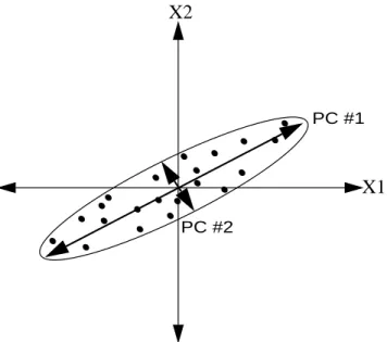
Graphical interpretation of principal components analysis is found in Figure 2-4. In this example there are two normal random variables (x1and x2) measured on a collection of samples. When plotted in two dimensions, it is apparent that the samples are correlated and can be enclosed by an ellipse. It is also apparent that the samples vary more along one axis (semi-major axis) of the ellipse than along the other (semi-minor axis). From the cor-relation between the two variables, it seems that the knowledge of one variable provides substantial (and perhaps sufficient) information about the other variable. Therefore, moni-toring the first principal component could give us most of the information about what is going on in the process, where by information in this context we mean the total variance. Furthermore, the second principal component can be thought of as a noise factor in the process, and one may chose to ignore or neglect it in comparison to the first principal com-ponent.
Figure 2-4: Graphical interpretation of PCA
2.5 SPC with Principal Components Analysis
With hundreds or thousands of measured variables, most recent multivariate SPC methods have been focused on multivariate statistical projection methods such as principal components analysis (PCA) and partial least squares (PLS). The advantages of projection methods are the same as those discussed in PCA. The key advantages include data reduc-tion, information extraction and noise filtering. These projection methods examine the behavior of the process data in the projection spaces defined by the reduced order model, and provide a test statistic to detect abnormal deviations only in the space spanned by a subset of principal components or latent variables. Therefore, projection methods must be used with caution so that these methods can keep track of unusual variation inside the model as well as unusual variation outside the model (where a model is defined by the
PC #1
PC #2
X1 X2
number of principal components retained). The projection methods are especially useful when the data is ill conditioned since the filtering throws out the ill conditioned part of the data. Ill conditioning occurs when there is exact or almost linear dependency among the variables; more details of such condition will be discussed in Section 2.6.1.
The multivariate T2statistic can then be combined with PCA to produce just one con-trol chart for easily detecting out of concon-trol sample points on a reduced dimension pro-vided by the PCA model. Let us assume that k out of p principal components are kept for the PCA model. Because of the special mapping of PCA, each PC is orthogonal to every other. Therefore, T2is computed as the sum of normalized squared scores from the k prin-cipal components and it is a measure of the variation from each sample within the PCA model from the k principal components. It is calculated based on the following formula
where si is the standard deviation associated with ti.
However, in order to identify the underlying causal variables for a given deviation, one needs to go back to the loadings or eigenvectors of the covariance matrix. First, from the T2value of the out of control point, we can find the contribution from each score by plot-ting the normalized scores from , where k is the number of principal com-ponents kept in the model and is the standard deviation associated with the i-th principal component (see [KM96]). Control limits such as Bonferroni limits can then be used on the chart as rough guidelines for detecting large values. Once the dominant scores are determined, one can then identify the key contributing variables on those
T2 ti s i ---- 2 i = 1 k
∑
= T2 ti si ---- 2 i= 1 k∑
= Si t i s i----scores. From principal components analysis, the scores are given by the following for-mula, where is the eigenvector corresponding the i-th principal component and X is the mean-centered data matrix.
(Eq. 2-2)
The above equation provides the contribution of each variable xjto the scores of the i-th principal component as .
Aside from tracking a T2statistic within the space spanned by PCA model, one must also pay attention to the residual between the actual sample and its projection onto the PCA model. The Q statistic does this [WRV90]; it is simply the sum of squares of the error:
(Eq. 2-3)
The Q statistic indicates how well each sample conforms to the PCA model.
Figure 2-5: Graphical interpretation of T2 and Q statistics
vi ti = Xvi v i j, xj Q = x xT–xV VTxT = x I( –V VT)xT X2 X3 X 1 Sample with large T2 Sample with large Q value PC #1 PC #2 o x
Figure 2-5 provides graphical interpretation of principal components analysis, T2and Q statistics. Though the data resides in a 3-D environment, most of the data, except one sample (point x), lie in a plane formed by the vectors of PC #1 and PC #2. As a result, a PCA model with two principal components adequately describes the process/data. The geometrical interpretation of T2 and Q is also shown in the figure. In this case, T2 is a squared statistical distance within the projection plane (see o point). On the other hand, Q is a measure of the variation of the data outside of the principal components defined by the PCA model. From the figure, Q is the squared statistical distance of the x point (see Eq. 2-3) off the plane containing the ellipse. Also note, a point can have a small T2 value because its projection is well within the covariance structure, yet its Q value can be large as for the point x in Figure 2-5.
2.6 Linear Regression Analysis Tools
In many design of experiment setups, we wish to investigate the relationship between a process variable and a quality variable. In some cases, the two variables are linked by an exact straight-line relationship. In other cases, there might exist a functional relationship which is too complicated to grasp or to describe in simple terms (see [Bro91] and [DS81]). In this scenario we often approximate the complicated functional relationship by some simple mathematical function, such as linear functions, over some limited ranges of the variables involved. The variables in regression analysis are distinguished as predictor/ independent variables and response/dependent variables. In this section, we briefly give some background information on some popular regression tools. While this thesis focuses on correlation structures within a set of input or output data (rather than between input and
Our detection methods make heavy use of PCA and eigenspace methods, and some back-ground is provided in this section on related regression methods so that the reader may understand the increasing importance of such eigenspace approaches in emerging data rich quality control environments.
The linear regression equations express the dependent variables as a function of the independent variables in the following way:
(Eq. 2-4)
where Y denotes the matrix of response variables and X is the matrix of predictor vari-ables. The error,ε,is treated as a random variable whose behavior is characterized by a set of distribution assumptions.
2.6.1 Linear Least Squares Regression
The first approach we review is linear least squares regression. The objective is to select a set of coefficientsβsuch that the Euclidean norm (also known as 2-norm) of the discrepancies is minimized. In other words, let S(β) be the sum of squared differences, . Thenβis chosen by searching through all possible
β to minimize S(β); this optimization is also known as the least squares criterion and its estimate is known as the least squares estimate ([DS81], [FF93]). Solution to this optimi-zation can be solved using the normal equation. Let b be the least squares estimate ofβ. We then can use the fact that the error vector ( ) is orthogonal to the vector sub-space spanned by X. Therefore, the solution is given by
(Eq. 2-5)
Least squares methods can be modified easily to weighted least squares, where weights are placed on different measurements. Such a weighting matrix is desirable when
Y = Xβ ε+
ε = Y–Xβ
S( )β = (Y–Xβ)T(Y X– β)
e = Y Xb–
the variances across different measurements are not the same, i.e. some prior information on the measurement can be included in the weighting matrix.
The least squares estimate requires that XTX be invertible; this might not be always
the case. In the case when a column of the predictor matrix X can be expressed as a linear combination of the other columns of X, XTX becomes singular and its determinant is zero.
When dependencies hold only approximately, the matrix of XTX becomes ill conditioned
giving rise to what is known as the multicollineartiy problem (see [DS81] and [Wel00]). With massive amount of data, it is very possible that redundancy or high correlation exits among variables, hence multicollinearity becomes a serious issue in data rich environ-ments.
2.6.2 Principal Components Regression
As its name suggests, the foundation of Principal Components Regression (PCR) is based on principal components. PCR is one of many regression tools that overcome the problem of multicollinearity. Multicollinearity occurs when linear dependencies exist among process variables or when there is not enough variation in some process variable. If that is the case, such variables should be left out since they contain no information about the process. One advantage of using principal components is that because all PCs are orthogonal to each other, multicollinearity is not an issue. Moreover, in PCA the variance equals information; so principal components with small variances can be filtered out and only a subset of the PCs are used as predictors in the matrix X. Using the loading matrix V as a coordinate transformation, the resulting equation for PCR is
(Eq. 2-6)
puted using the least squares estimate equation in Eq. 2-5, i.e. .
The analysis above is done around principal components, namely Z’s. Though we can reduce the number of PCs in the analysis, all the original X variables are still present and none is eliminated by the above procedure. Ideally, one would like to eliminate those input variables in X which do not contribute to the model, so some sort of variables selection procedure can be done prior to the regression procedure.
2.6.3 Partial Least Squares
Partial Least Squares (PLS) has also been used in ill conditioned problems encoun-tered in massive data environments. While PCA finds factors through the predictor vari-ables only, PLS finds factors from both the predictor varivari-ables and response varivari-ables. Because PCA finds factors that capture the greatest variance in the predictor variables only, those factors may or may not have any correlation with the response variables. Because the purpose of regression is to find a set of variables that best predict the response variables, it is desirable then to find factors that have strong correlation with the response variables. Therefore, PLS finds factors that not only capture variance of predictor vari-ables but also achieve correlation to the response varivari-ables. That is why PLS is described as a covariance maximizing technique ([FF93], [LS95]). PLS is a technique that is widely used in chemometrics applications.
There are several ways to compute PLS, however, the most instructive method is known as NIPLS for Non-Iterative Partial Least Squares. Instead of one set of loadings in PCR, there are two sets of loadings used in PLS, one for the input matrix and one for the response variables. The algorithm is described in the following steps:
1. Initialize: Pick Y0=Y, X0=X
2. For i=1 to p do the following
3. Find i-th covariance vector of X0 and Y0 data by computing
4. Find i-th scores of X data by computing
5. Estimate the i-th input loading
6. Compute the i-th response loadings
7. Set and
8. End of loop.
From the vectors wi, ti and pi found above, matrices of W, T and P are formed by
and the PLS estimate ofβ is
2.6.4 Ridge Regression
Ridge regression is intended to overcome multicollinearity situations where correla-tions between the various predictors in the model cause the XTX matrix to be close to
sin-gular, giving rise to unstable parameter estimation. The parameter estimates in this case may either have the wrong sign or be too large in magnitude for practical consideration [DS81]. wi Xi–1 T Yi–1 Xi–1 T Yi–1 ---= ti = Xi–1wi pi Xi–1 T ti ti ---= qi Yi–1 T ti ti ---= Xi Xi–1 tipi T – = Yi = Yi–1–tiqi W w1 w2 … wp, T t1 t2 … tp , P= p1 p2 … pp ˙ = = β = W P( TW)–1(TTT)–1TTY
Let the data X be mean-centered (so one does not include the intercept term). The esti-mates of the coefficients in Eq. 2-4 are taken to be the solution of a penalized least squares criterion with the penalty being proportional to the squared norm of the coefficientsβ:
(Eq. 2-7)
The solution to the problem is
The only difference between this and the solution to the least squares estimate is the addi-tive termγI. This term stabilizes XTX, which then becomes invertible.γis a positive num-ber and in real applications the interesting values ofγ are in the range (0,1).
We can examine ridge regression from the principal components perspective [Wel00]. In order to do so, we need to express XTX in terms of principal components
where n is the number of observations. Then can be expressed as the follow-ing
(Eq. 2-8)
Eq. 2-8 provides some insight into the singular values of in terms of the sin-gular values of . Through ridge regression, the i-th singular value has been modi-fied from to (Eq. 2-9) b arg inm β E Y( –Xβ) 2 γ βT β + [ ] = b( )γ = (XTX+γI)–1XTY S X T X n–1 --- VΛVT⇒XTX (n–1)VΛV˙T = = = XTX+γI ( )–1 XTX+γI ( )–1 n 1– ( )VΛVT+γV VT [ ]–1 V[(n–1)Λ γ+ I]–1VT = = XTX+γI ( )–1 XTX ( )–1 1 n–1 ( )λi ---1 n–1 ( )λi+γ
---From Eq. 2-9, if λi is large, then dominates over γ and becomes
. Whenλiis small (almost zero), then γdominates over and
becomes . Finally, the key difference between PCR and ridge regression is that PCR removes principal components with small eigenvalues (near zero), whereas ridge regres-sion compensates the eigenvalues of those principal components byγ.
n–1 ( )λi 1 n–1 ( )λi+γ ---1 n–1 ( )λi --- (n–1)λi 1 n–1 ( )λi+γ ---1 γ
---Chapter 3
Second Order Statistical Detection: An
Eigenspace Method
3.1 Introduction
The goal of this chapter is to introduce two new multivariate detection methods, an eigenspace and a Cholesky decomposition detection method, as well as their fundamental properties. Before introducing these new multivariate detection methods, we need to establish certain terminology that will be used throughout the thesis. These terms are sometimes defined differently according to the field of discipline, and we must be clear on our usage so that confusion will not arise in the following sections.
We then revisit all SPC methods mentioned in the previous chapter and discuss advan-tages and disadvanadvan-tages associated with each method. Graphical and concrete examples are provided to enhance the understanding of what each detection method can do and can not do. Moreover, because the focus is on second order statistics, most of the examples provided in this chapter have to do with covariance/correlation shift and the goal is to detect such change in the examples. Motivation for a new multivariate detection method is then addressed. The new eigenspace detection method capable of detecting subtle covari-ance structure changes is then defined and specific multivariate examples are provided to illustrate the advantages of this new method.
Mathematical properties of the eigenspace detection method are derived. In particular, these properties include the distribution of the test statistic provided by the eigenspace
detection method and key asymptotic properties on this distribution. These properties are important, as control limits must be established for event detection using the new eigens-pace detection method, and these limits of course depend strongly on the distribution of the new statistic.
3.2 First Order Statistical and Second Order Statistical Detection
Meth-ods
Almost all modern SPC methods are based on hypothesis testing. In practice, an inde-pendent normally distributed assumption is placed on the data. Moreover, data collected is placed in the matrix form X defined in Section 2.3. Basic descriptive statistics such as sample mean and sample variance can then be computed from the random samples in X. Some of the descriptive statistics use only the first moment and are called first order statis-tics. Other descriptive statistics compute the second moment from the sample and are called second order statistics. Finally, these sample statistics are used in the hypothesis testing to arrive at a conclusion as to whether or not these data samples could be coming from a known distribution.
3.2.1 First Order Statistical Detection Methods
Before we discuss the definition of first order statistical detection methods, let us establish terminology for single sample and multiple sample detection methods. Single sample detection collects one sample at a time and a test statistic can then be computed from the sample; that statistic is then used to conclude if the sample conforms with the past data. Multiple sample detection methods use sample statistics computed from several samples for a hypothesis test.
In this section, we provide detailed discussion to distinguish a multivariate first order detection method from a multivariate second order detection method. First order detection methods extract only a first order statistic or first moment from a future sample or samples and use that first order statistic or moment to make inferences about some known parame-ters. However, the known parameters can include higher order statistics computed from the training or past data. We want to emphasize that the order of a statistical detection method is defined based on the statistic derived from a test sample or samples, and does not directly utilize the trial or historical samples. In other words, first order statistical methods compare the first moment from the test samples to the subspace spanned by the training data and determine if the test samples could be generated from the training data population. Note that first order statistical detection methods can be either single sample or multiple sample detection methods.
The sample mean control chart is used extensively and is an example of a first order detection method. Basically, independent identically distributed test random samples of size m are collected, , and the sample mean is computed. Hypothesis testing can then be performed, and its alternative hypothesis is . We are trying to decide the probability that can be generated by a popula-tion whose mean isµ0. Bear in mind thatµ0is found from the historical data and is char-acterized as the population mean. Many hypothesis testing problems can be solved using the likelihood ratio test (see [JW98]). However, there is another more intuitive way of solving hypothesis testing problems, and it uses the concept of a statistical distance mea-sure. In the univariate scenario, has a student’s t-distribution and is the statisti-cal distance from the sample to the test valueµ0weighted by sample standard deviation s.
X X1 X2 … Xi … Xm T = X H0: X = µ0 H1: X≠µ0 X t (x–µ0) s ---=
By analogy, T2 is a generalized statistical squared distance from x to the test vector µ0,
defined to be
The T2statistic is also known as Hotelling’s T2. Since it is a distance measure, if T2is too large, then x is too far fromµ0, hence the null hypothesis is rejected. Thus a standard T2statistic is a single sample first order detection method where T2is calculated based on a single new data point.
3.2.2 Second Order Statistical Detection Methods
In order to compute second order statistics, multiple samples (more than one sample) must be collected from the test data. Hence, second order statistics or moments are extracted from these samples and inferences can then be carried out using hypothesis test-ing. A well known second order statistic widely used in univariate SPC is the S (standard deviation) chart. In practice, the R (range) chart is often used, especially when the sample size is relatively small. Moreover, an estimate of standard deviation can be computed from the sample range R [Mon91]. In multivariate data, individual S or R charts can be moni-tored when the dimension of the data is small. However, the problem becomes non-tracta-ble when the data dimension increases rapidly as in modern data rich environments.
A widely used measure of multivariate dispersion is the sample generalized variance. The generalized variance is defined to be the determinant of the covariance matrix. This measure provides a way of compressing all information provided by variances and covari-ances into a single number. In essence the generalized variance measure is proportional to
the square of the volume spanned by the vectors in the covariance matrix [JW98], [Alt84], and can be thought of as a multidimensional variance volume.
Although the generalized variance has some intuitively pleasing geometrical interpre-tations, its weakness is similar to all descriptive summary statistics - lost information. In matrix algebra, several different matrices can generate the same determinant (that is, dif-ferent covariance structures may generate the same generalized variance), geometrical interpretation of this problem will be illustrated in Section 3.3.4. Mathematically, how-ever, we can see that the following three covariance matrices all have the same determi-nant:
, ,
Although each of these covariance matrices has the same generalized variance, they pos-sess distinctly different covariance structures. In particular, there is positive correlation between variables in S1and the correlation coefficient of S2is the same in magnitude as in
S1, but the variables in S2are negatively correlated. The variables in S3are independent of each other. Therefore, different correlation structures are not detected by the generalized variance. A better second order statistical detection method is desired which compares in more detail the subspace spanned by the test samples with the subspace generated by the training data, and this is the focus of this thesis.
3.3 Weaknesses and Strengths in Different Detection Methods
3.3.1 Univariate SPC
The weakness of univariate SPC applied on multivariate data is discussed in
S1 5 4 4 5 = S2 5 –4 4 – 5 = S3 3 0 0 3 =
Section 2.2.1, and an example is illustrated in that section. Although univariate SPC is easy to use and monitor, it should only be used when the dimension of the data is small. Moreover, the correlation information is essential in multivariate analysis, yet univariate SPC does not use that information.
3.3.2 Multivariate SPC First Order Detection Methods (T2)
The T2 has been used extensively due to its attractive single value detection scheme using the generalized distance measure. The advantage of using the T2 statistic is that it compresses all individual control charts on xi into a single control chart as well as keeps track of the correlation information among variables. The power of T2based detection can be boosted when multiple samples are collected; this is a direct result of the sample mean. As n increases, the variance of sample mean decreases as . Therefore, one can always resolve two populations with different means using a T2 detection method with large enough n.
There are some computational issues related to T2 methods. When data dimension increases, the multicollinearity issue can not be overlooked. Collinearity causes the covari-ance matrix to be singular, hence T2can not be computed. There are some ways to work around the problem: one can compute the Moore-Penrose generalized inverse, which is also known as the pseudo inverse. The covariance matrix also becomes non-invertible when the number of sequential samples collected exceeds the data dimension.
As with most of the data compression methods, T2 gains from compression but also suffers from compression, i.e. because of compression some key information is lost. The generalized distance loses information on directionality, as depicted in Figure 3-1. In this
1
n
---and those on the right; they all have a large T2 value.
Figure 3-1: T2 statistic drawback
Therefore, T2 is suitable if the purpose is only to detect out-of-control events. Second order statistical methods might be desirable when the lost information such as directional-ity can be used for both event detection and classification, or for process improvement pur-poses.
3.3.3 PCA and T2 methods
PCA provides great advantage for data compression: instead of dealing with hundreds of variables, we are now dealing with a few principal components. However, the T2 statis-tic only tracks the data in the projection hyperplane; one must also track the Q statisstatis-tic in order to detect if the PCA model no longer describes the process. PCA and T2suffer the same problem as T2 does; it is a type of statistical distance measure, so it can not resolve