Data Assimilation with Gaussian Mixture Models
using the Dynamically Orthogonal Field Equations
by
~MASSACHUSETTS ITITUTEOF TECTHNOLOGY
Thomas Sondergaard
M.Eng., Imperial College of London (2008)
17,3
Submitted to the Department of Mechanical Engineering
ARCHIVES
in partial fulfillment of the requirements for the degree of
Master of Science in Mechanical Engineering
at the
MASSACHUSETTS INSTITUTE OF TECHNOLOGY
September 2011
©
Massachusetts Institute of Technology 2011. All rights reserved.
A uthor ...
...
/
Department of Mechanical Engineering
08/03/2011
Certified by.
Ass iate
Pierre F. J. Lermusiaux
Professor of Mechanical Engineering
Thesis Supervisor
A ccepted by ...
...
David E. Hardt
Chairman, Department Committee on Graduate Theses
Data Assimilation with Gaussian Mixture Models using the
Dynamically Orthogonal Field Equations
by
Thomas Sondergaard
Submitted to the Department of Mechanical Engineering on 08/03/2011, in partial fulfillment of the
requirements for the degree of
Master of Science in Mechanical Engineering
Abstract
Data assimilation, as presented in this thesis, is the statistical merging of sparse observational data with computational models so as to optimally improve the prob-abilistic description of the field of interest, thereby reducing uncertainties. The cen-terpiece of this thesis is the introduction of a novel such scheme that overcomes prior shortcomings observed within the community. Adopting techniques prevalent in Machine Learning and Pattern Recognition, and building on the foundations of classical assimilation schemes, we introduce the GMM-DO filter: Data Assimilation with Gaussian mixture models using the Dynamically Orthogonal field equations.
We combine the use of Gaussian mixture models, the EM algorithm and the Bayesian Information Criterion to accurately approximate distributions based on Monte Carlo data in a framework that allows for efficient Bayesian inference. We give detailed descriptions of each of these techniques, supporting their application
by recent literature. One novelty of the GMM-DO filter lies in coupling these
con-cepts with an efficient representation of the evolving probabilistic description of the uncertain dynamical field: the Dynamically Orthogonal field equations. By limiting our attention to a dominant evolving stochastic subspace of the total state space, we bridge an important gap previously identified in the literature caused by the dimen-sionality of the state space.
We successfully apply the GMM-DO filter to two test cases: (1) the Double Well Diffusion Experiment and (2) the Sudden Expansion fluid flow. With the former, we prove the validity of utilizing Gaussian mixture models, the EM algorithm and the Bayesian Information Criterion in a dynamical systems setting. With the application of the GMM-DO filter to the two-dimensional Sudden Expansion fluid flow, we further show its applicability to realistic test cases of non-trivial dimensionality. The
GMM-DO filter is shown to consistently capture and retain the far-from-Gaussian statistics
that arise, both prior and posterior to the assimilation of data, resulting in its superior performance over contemporary filters.
We present the GMM-DO filter as an efficient, data-driven assimilation scheme, focused on a dominant evolving stochastic subspace of the total state space, that
respects nonlinear dynamics and captures non-Gaussian statistics, obviating the use of heuristic arguments.
Thesis Supervisor: Pierre F. J. Lermusiaux
Acknowledgments
I would like to extend my gratitude to my adviser, Pierre Lermusiaux, for having
given me the complete freedom to pursue a thesis topic of my own interest. I am further appreciative of the kind understanding he has shown me, particularly in the months leading up to this deadline. His helpful comments, guidance and support have aided in producing a thesis of which I am truly proud.
My most sincere thanks also go to the rest of the MSEAS team, both past and
present. Particularly, I wish to thank the members of my office, who have been a family away from home!
I finally wish to acknowledge my family, whose help and support has been invalu-able. It is due to them that I have been given the opportunity to pursue a degree at MIT; from them that I have gained my curiosity and desire to learn; and whose values have defined the person that I am.
Contents
1 Introduction 1.1 B ackground . . . . 1.2 G oals . . . . . . . .. 1.3 Thesis Overview. . . . . 2 Data Assimilation 2.1 Kalman Filter . . . . 2.2 Extended Kalman Filter . . . .2.3 Ensemble Kalman Filter . . . . 2.4 Error Subspace Statistical Estimation . . . .
2.5 B ayes F ilter . . . .
2.6 P article F ilter . . . .
3 Data Assimilation with Gaussian mixture models using the Dynam-ically Orthogonal field equations
3.1 Gaussian mixture models . . . .
3.2 The EM algorithm . . . .
3.2.1 The EM algorithm with Gaussian mixture models
3.2.2 R em arks . . . .
3.3 The Bayesian Information Criterion . . . . 3.4 The Dynamically Orthogonal field equations . . . . 3.4.1 Proper Orthogonal Decomposition . . . . 3.4.2 Polynomial Chaos . . . . 7 17 17 18 18 21 22 30 34 37 38 40 43 44 49 53 60 61 65 66 66
3.4.3 The Dynamically Orthogonal field equations . . . . 67
3.5 The GMM-DO filter . . . . 70
3.5.1 Initial Conditions . . . . 70
3.5.2 Forecast . . . . 72
3.5.3 Observation . . . . 73
3.5.4 U pdate . . . . 73
3.5.5 Exam ple . . . . 82
3.5.6 Remarks, Modifications and Extensions . . . . 88
3.6 Literature Review . . . . 91
4 Application 1: Double Well Diffusion Experiment 101 4.1 Introduction . . . 101
4.2 Procedure .. .. ... ... ... . . . . . . 104
4.3 Results and Analysis . . . 106
4.4 C onclusion . . . 119
5 Application 2: Sudden Expansion Fluid Flow 121 5.1 Introduction . . . . 122
5.2 P rocedure . . . 125
5.3 Numerical Method . . . 128
5.4 Results and Analysis . . . 130
5.5 C onclusion . . . 158
6 Conclusion 159 A Jensen's Inequality and Gibbs' Inequality 161 B The covariance matrix of a multivariate Gaussian mixture model 165 C Maximum Entropy Filter 167 C.1 Formulation . . . 167
List of Figures
3-1 Gaussian (parametric) distribution, Gaussian mixture model and Gaus-sian (kernel) density approximation of 20 samples generated from the mixture of uniform distributions: px(x) = x U(X; -- 8, -1) + j x
U(x; 1, 8), where U(x; a, b) = denotes the continuous uniform prob-ability density function for random variable X . . . . 45
3-2 GMM-DO filter flowchart. . . . . 83
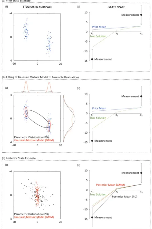
3-3 GMM-DO filter update. In column (i), we plot the set of ensemble real-izations within the stochastic subspace,
{};
in column (ii), we display the information relevant to the state space. Panel (a) shows the prior state estimate; in panel (b), we show the fitting of Gaussian mixture models of complexity M = 1 (PD) and M = 2 (GMM), and plot their marginal distributions for each of the stochastic coefficients; in panel (c), we provide the posterior state estimate again in the decomposed form that accords with the D.O. equations. . . . . 873-4 Schematic representation of advantages of kernel over single Gaussian filter for a low-order model. The background is a projection of a trajec-tory from the Lorenz-63 model showing the attractor structure. Super-imposed is an idealized image of the single Gaussian (outer curve) and kernel (inner curves) prior distributions for a three-member ensemble.
4-1 Forcing Function, f(x). At any location (o), x, the ball is forced under pseudo-gravity in the direction indicated by the appropriate vector. The magnitude of the vector corresponds to the strength of the forcing. We note that there exists an unstable node at the origin, and two stable nodes at x = t1, corresponding to the minima of the wells. . . . 102 4-2 Climatological distribution and Gaussian mixture approximation for
, = 0.40. In accordance with intuition, the distributions are bimodal,
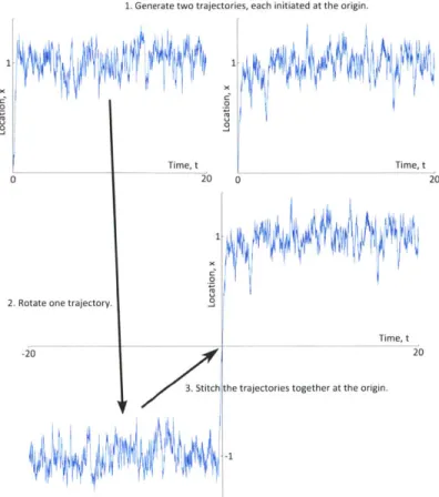
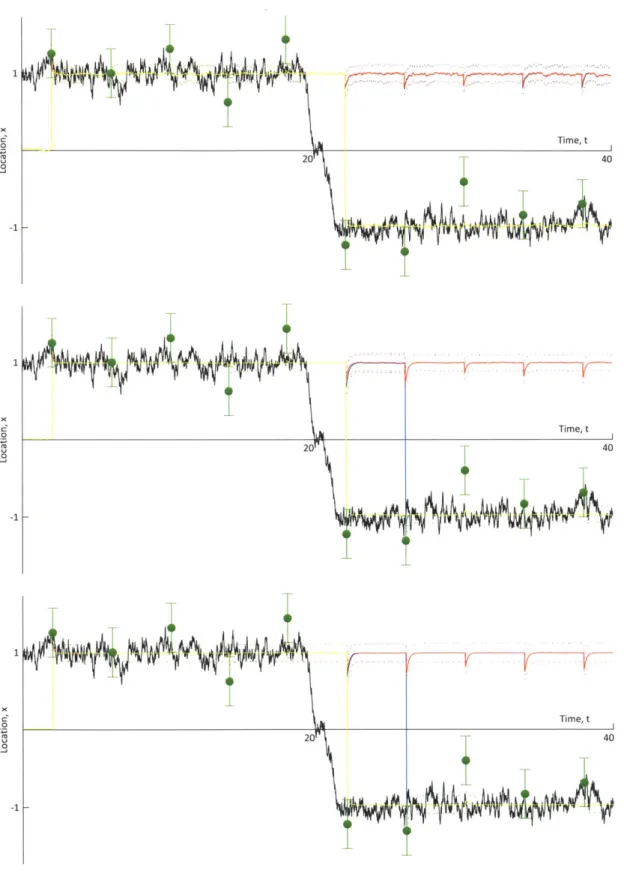
appropriately centered on the minima of each of the two wells. . . . . 103 4-3 Example trajectory of the ball for K = 0.45. The horizontal axis
de-notes time; the vertical axis the location of the ball. Superimposed onto the plot are intermittent measurements, shown in green, with their associated uncertainties. . . . 104 4-4 The true trajectory for the ball is obtained by appropriately stitching
together two runs, each initiated at x = 0. . . . 105 4-5 Legend for the Double Well Diffusion Experiment. . . . 106 4-6 Results for MEF, GMM-DO, and EnKF with parameters r, 0.4; 0f =
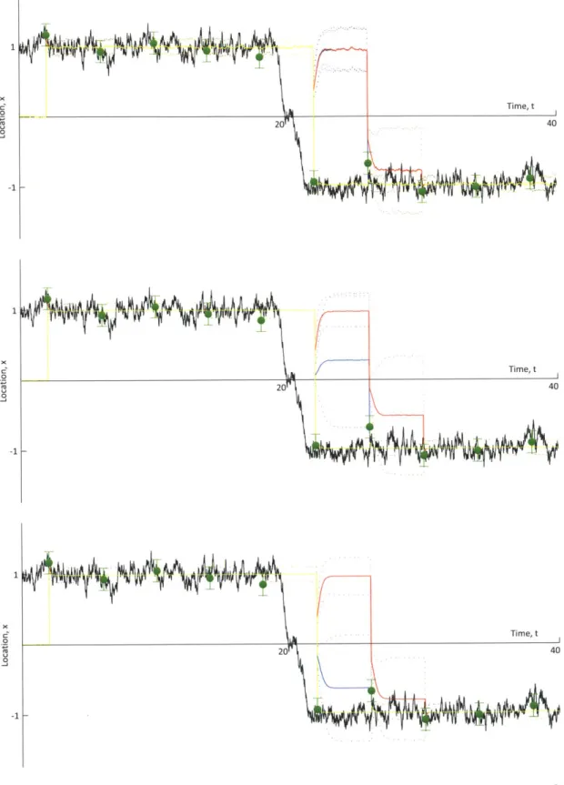
0.025; and (top) 100 particles; (middle) 1000 particles; and (bottom) 10000 particles. . . . 107
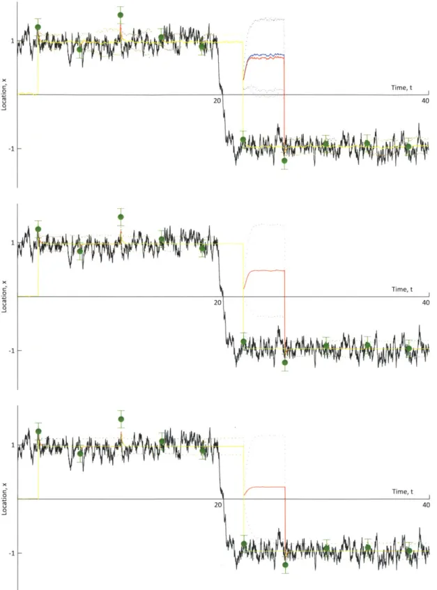
4-7 Results for MEF, GMM-DO, and EnKF with parameters , = 0.4; 0,2 0.050; and (top) 100 particles; (middle) 1000 particles; and (bottom) 10000 particles. . . . 108
4-8 Results for MEF, GMM-DO, and EnKF with parameters , = 0.4; o0 =
0.100; and (top) 100 particles; (middle) 1000 particles; and (bottom) 10000 particles. . . . 109
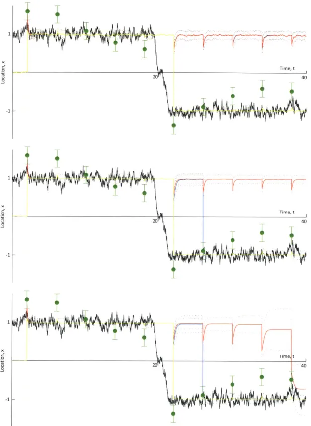
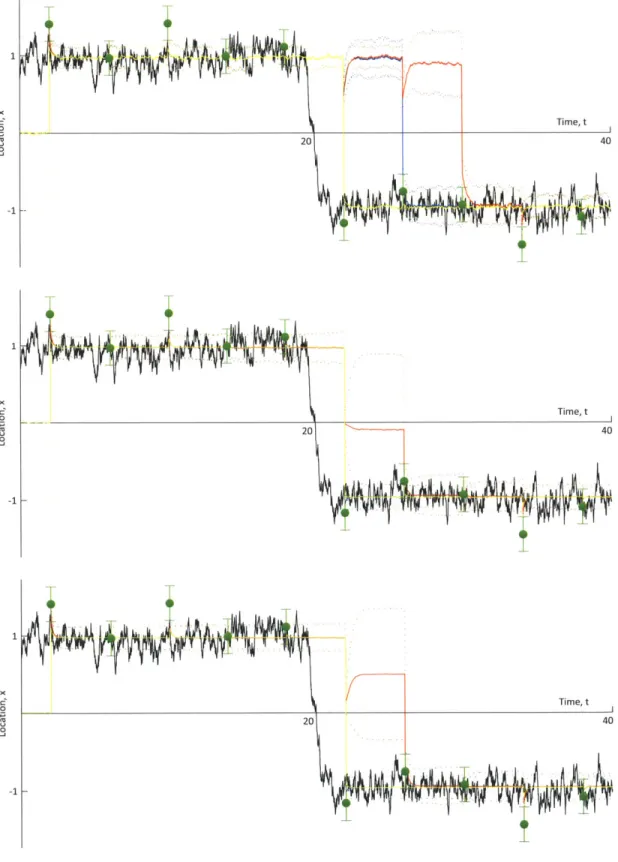
4-9 Results for MEF, GMM-DO, and EnKF with parameters K = 0.5; Oj -0.025; and (top) 100 particles; (middle) 1000 particles; and (bottom)
10000 particles. . . . 110
4-10 Results for MEF, GMM-DO, and EnKF with parameters K = 0.5; U2 =
0.050; and (top) 100 particles; (middle) 1000 particles; and (bottom) 10000 particles. . . . .111
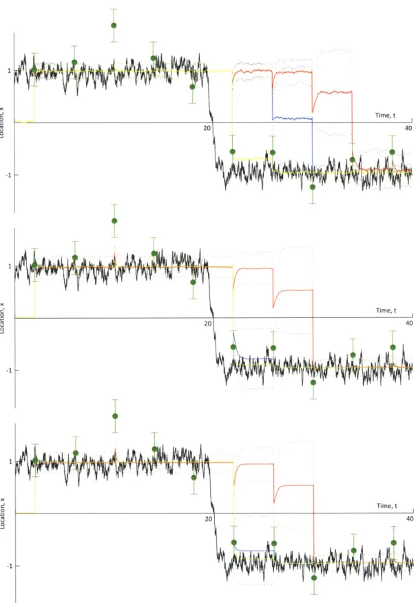
4-11 Results for MEF, GMM-DO, and EnKF with parameters , = 0.5; o =
0.100; and (top) 100 particles; (middle) 1000 particles; and (bottom)
10000 particles. . . . . 112
4-12 Analysis of the prior and posterior distributions (and particle repre-sentations) by each of the three filters (EnKF, GMM-DO and MEF) for the particular case of N = 1, 000 and i = 0.5, centered on the observation immediately prior to the true transition of the ball. . . . 115
4-13 Analysis of the prior and posterior distributions (and particle repre-sentations) by each of the three filters (EnKF, GMM-DO and MEF) for the particular case of N = 1, 000 and r = 0.5, centered on the observation immediately following the true transition of the ball. . . . 116
4-14 Analysis of the prior and posterior distributions (and particle represen-tations) by each of the three filters (EnKF, GMM-DO and MEF) for the particular case of N = 1, 000 and K = 0.5, centered on the second observation following the true transition of the ball.. . . . . . 117
5-1 Setup of the sudden expansion test case (Fearn et al., 1990). . . . . . 122
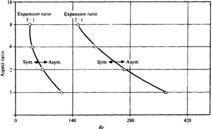
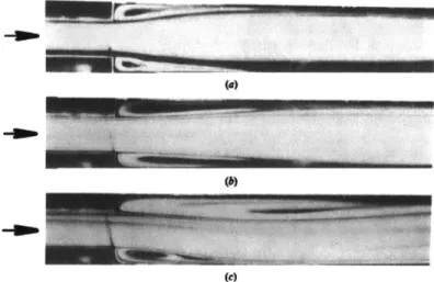
5-2 Boundaries of symmetric and asymmetric flow as a function of aspect ratio, expansion ratio and Reynolds number (Cherdron et al., 1978). . 123 5-3 Flow patterns at different Reynolds numbers for an aspect ratio of 8 and an expansion ratio of 2. (a) Re = 110. (b) Re = 150. (c) Re = 500. (Cherdron et al., 1978). . . . . 124
5-4 Numerical and experimental velocity plots at Re = 140. The numer-ically calculated profiles are shown as continuous curves. (a) x/H = 1.25; (b) x/H = 2.5; (c) x/H = 5; (d) x/H = 10; (e) x/H = 20; (f) x/H = 40. (Fearn et al., 1990). . . . . 124
5-5 Calculated streamlines at Re = 140. (Fearn et al., 1990). . . . . 124
5-6 Sudden Expansion Test Setup. . . . . 125
5-7 Initial mean field of the DO decomposition. . . . . 126
5-9 Observation Locations: (Xobs, Yobs) {(4, - (4, 0), (4, )}..
5-10 True solution; condensed representation
root mean square errors at time T = 0. .
5-11 True solution; condensed representation
root mean square errors at time T = 10.
5-12 True solution; condensed representation
root mean square errors at time T = 20.
5-13 True solution; condensed representation
root mean square errors at time T = 30. 5-14 True solution; condensed representation
root mean square errors at time T = 40.
of DO decomposition; and of DO of DO of DO of DO decomposition; decomposition; decomposition; decomposition;
5-15 True solution; DO mean field; and first four DO modes at the first
assimilation step, time T = 50 .. . . . .
5-16 True solution; DO mean field; and joint and marginal prior
distribu-tions, identified by the Gaussian mixture model of complexity 29, and associated ensembles of the first four modes at the first assimilation step, tim e T = 50 .. . . . .
5-17 True solution; observation and its associated Gaussian distribution;
and the prior and posterior distributions at the observation locations at tim e T = 50. . . . .
5-18 True solution; condensed representation of the posterior DO
decompo-sition; and root mean square errors at time T = 50. . . . .
5-19 True solution; condensed representation of DO decomposition; and
root mean square errors at time T = 60. . . . .
5-20 True solution; DO mean field; and first four DO modes at the second
assimilation step, time T = 70 .. . . . .
5-21 True solution; DO mean field; and joint and marginal prior
distribu-tions, identified by the Gaussian mixture model of complexity 20, and associated ensembles of the first four modes at the second assimilation step, tim e T = 70 .. . . . . 129 132 133 134 135 and and and and . . . . 136 137 138 139 140 141 142 143
5-22 True solution; observation and its associated Gaussian distribution;
and the prior and posterior distributions at the observation locations at time T = 70... . . . . . . . . 144
5-23 True solution; condensed representation of posterior DO
decomposi-tion; and root mean square errors at time T = 70. . . . . 145
5-24 True solution; condensed representation of DO decomposition; and root mean square errors at time T = 80. . . . . 146
5-25 True solution; DO mean field; and first four DO modes at the third
assimilation step, time T = 90 . . . . 147
5-26 True solution; DO mean field; and joint and marginal prior
distribu-tions, identified by the Gaussian mixture model of complexity 14, and associated ensembles of the first four modes at the third assimilation step, tim e T = 90 . . . . 148
5-27 True solution; observation and its associated Gaussian distribution;
and the prior and posterior distributions at the observation locations at tim e T = 90. . . . .. 149
5-28 True solution; condensed representation of posterior DO
decomposi-tion; and root mean square errors at time T = 90. . . . . 150
5-29 True solution; condensed representation of DO decomposition; and
root mean square errors at time T = 100. . . . . 151
5-30 Time-history of the root means square errors for the GMM-DO filter
and DO-ESSE Scheme A. . . . . 152
5-31 Bimodal distribution for the most dominant stochastic coefficient, <bi,
at T = 40. The GMM-DO filter captures and retains this bimodality throughout the simulation of the sudden expansion fluid flow, resulting in its superior performance. . . . . 153
5-32 Gaussian mixture model approximation of the ensemble set,
{<p},
at the time of the first assimilation of observations, T - 50. Assuming MAT-LAB's 'ksdensity' function to represent an appropriate approximation to the true marginal densities, we note the satisfactory approximation of the Gaussian mixture model. . . . 1545-33 An example of the manner in which the GMM-DO filter captures the
true solution through its use of Gaussian mixture models. We equally note the increased weights placed on the mixtures surrounding the true solution following the Bayesian update, depicted by the green curve. . 155 5-34 A second example of the manner in which the GMM-DO filter captures
the true solution through its use of Gaussian mixture models. Here, however, the true solution is contained within a mode of small - but finite - probability. Note the increased weights placed on the mixtures surrounding the true solution following the Bayesian update. . . . 156
5-35 We show the part of the true solution orthogonal to the stochastic
subspace for the case of 15 and 20 modes at the time of the first assim-ilation. 'Difference' refers to the difference between the true solution and the mean field; 'error' to the part of the true solution not cap-tured by the GMM-DO filter. We note that as we increase the number of modes, the norm of the error marginally decreases, indicative of
Chapter 1
Introduction
1.1
Background
The need for generating accurate forecasts, whether it be for the atmosphere, weather or ocean, requires little justification and has a long and interesting history
(see e.g. Kalnay (2003)). Such forecasts are, needless to say, provided by highly developed and complex computational fluid dynamics codes. An example of such is that due to MSEAS (Haley and Lermusiaux (2010); MSEAS manual) .
Due to the chaotic nature of the weather and ocean, however, classically exemplified by the simple Lorenz63 model (Lorenz, 1963), any present state estimate -however accurate - is certain to deteriorate with time. This necessitates the assimila-tion of external observaassimila-tions. Unfortunately, due to the limitaassimila-tion of resources, these are sparse in both space and time. Given further the dimensionality of the state vector associated with the weather and ocean, a crucial research thrust is thus the efficient distribution of the observational information amongst the entire state space.
Data assimilation concerns the statistical melding of computational models with sparse observations for the purposes of improving the current state representation.
By arguing that the most complete description of any field of interest is its probability
distribution, the ultimate goal of any data assimilation scheme is the 'Bayes filter', to be introduced in this thesis. The scheme to be developed in this thesis is no different.
1.2
Goals
The centerpiece of this thesis is the introduction of a novel data assimilation scheme that overcomes prior shortcomings observed within the data assimilation com-munity. Adopting techniques prevalent in Machine Learning and Pattern Recognition, and building on the foundations of the Kalman filter (Kalman) and ESSE (Lermu-siaux, 1997), we introduce the GMM-DO filter: Data Assimilation with Gaussian mixture models using the Dynamically Orthogonal field equations. By application of the Dynamically Orthogonal field equations (Sapsis (2010), Sapsis and Lermusi-aux (2009)), we focus our attention on a dominant evolving stochastic subspace of the total state space, thereby bridging an important gap previously identified in the literature caused by the dimensionality of the state space. Particularly, with this, we make obsolete ad hoc localization procedures previously adopted - with limited success - by other filters introduced in this thesis. With the GMM-DO filter, we
further stray from the redundant operating on ensemble members during the update step; rather, under the assumption that the fitted Gaussian mixture model accurately captures the true prior probability density function, we analytically carry out Bayes' Law efficiently within the stochastic subspace.
We describe the GMM-DO filter as an efficient, data-driven assimilation scheme that preserves non-Gaussian statistics and respects nonlinear dynamics, obviating the use of heuristic arguments.
1.3
Thesis Overview
In chapter 2, we explore various existing data assimilation schemes, outlining both their strengths and weaknesses. We will mainly limit our attention to methodologies based on the original Kalman filter (Kalman), whose general theory will serve as the
foundation for the GMM-DO filter.
In chapter 3, we will introduce the critical components that ultimately combine to produce the GMM-DO filter. After providing the details of the scheme itself, we will
give a simple example of its update step. We conclude the chapter with a literature review, in which we compare and contrast the GMM-DO filter against past and more recent schemes built on similar foundations.
In chapters 4 and 5, we apply the GMM-DO filter to test cases that admit far-from-Gaussian statistics. We specifically evaluate the performance of the GMM-DO filter when applied to the Double Well Diffusion Experiment (Chapter 4) and the Sudden Expansion fluid flow (Chapter 5), comparing its performance against that of contemporary data assimilation schemes. We describe in detail the manner in which the GMM-DO filter efficiently captures the dominant non-Gaussian statistics, ultimately outperforming current state-of-the-art filters.
Chapter 2
Data Assimilation
Data assimilation, as presented in this thesis, is the statistical merging of obser-vational data with computational models for the sake of reducing uncertainties and improving the probabilistic description of any field of interest. The concern will par-ticularly be with the aspect of filtering: generating the most complete description at present time, employing all past observations. In a future work, we may further extend this to the case of smoothing.
Today, ocean and weather forecasts are provided by computational models. In-evitably, these models fail to capture the true nature of the field of interest, be it due to discretization errors, approximations of nonlinearities, poor knowledge of parameter values, model simplifications, etc. As a consequence, one often resorts to providing a probabilistic description of the field of interest, introducing stochastic forcing, param-eter values and boundary conditions where necessary (Lermusiaux et al., 2006). By further incorporating uncertainties in the initial conditions, data assimilation goes be-yond providing a single deterministic estimate of the field of interest; rather, given the inherent uncertainties in both forecast and observations, data assimilation provides a statistical description from which one may quantify states and errors of interest.
The purpose of this chapter is to explore various traditional data assimilation schemes, outlining both their strengths and weaknesses. We will mainly limit our attention to methodologies based on the original Kalman filter, whose general theory will serve as the foundation for the data assimilation scheme to be developed in this
thesis.
The following presentation is largely based on the MSEAS thesis by Eric Heubel
(2008), the MIT class notes on Identification, Estimation and Learning by Harry
Asada (2011), chapter 22 of Introduction to Geophysical Fluid Dynamics by Cushman-Roisin and Beckers (2007), and the seminal books by Gelb (1974) and Jazwinski
(1970).
2.1
Kalman Filter
The Kalman filter (Kalman) merges model predictions with observations based on sound statistical arguments, utilizing quantified uncertainties of both predicted state variables and measurements. It is sequential in nature, essentially consisting of two distinct components performed recursively: a forecast step and an update step. While the structure of the update step will change little as we progress into more evolved filters, the forecast step of the Kalman filter specifically assumes linear dynamics. Particularly, we write for the discrete-time governing equation:
Xk+1 - AkXk + GkFk, (2.1)
where X
E
Rn is the (random) state vector; FkC
R' is a random vector (source of noise); k is a discrete time index; and Ak C R""" and Gk C R"" are matrices whosephysical interpretations require little clarification.
Sparse and noisy measurements of the system, Yk E RP, are intermittently col-lected, assumed to be a linear function of the state vector:
Yk = HkXk + Tk, (2.2)
where the vector Tk E RP represents measurement noise. The observation operator
Hk
C
RPXl linearly maps elements from the state space to the observation space,thus allowing their statistical comparison.
Particularly, the sources of noise are assumed to be unbiased:
E [i] = 0
E [Tt] =0
with the following auto- and cross-correlations in space and time:
S
[f
srT]
=6,Rt
. [rsT] = 0
where
ogj
denotes the Kronecker delta. With this, we proceed to examine the ma-chinery of the Kalman filter.Update
At any point in time, the goal of the Kalman filter is to determine the state vector,
Xa, that minimizes the quadratic cost function
X" = argmin E [ (X Xt) (X - zX) I yk, Xo],
x
(2.5)
where xz is the true state of the system; y' = {yi,. Yk} represents all measure-ments collected up to the current time step; and Xo is the initial state estimate. We refer to Xa as the analysis vector.
If we define the error A = X - x, with the assumption that this estimate is unbiased (i.e. S [A] = 0), we find that (2.5) is equivalent to writing
xa = argmin E [ATA I yk, X 0]
= argmin Tr (E [AAT I yk, X0])
(2.6) (2.7) (2.8)
=- argmin Tr () ,
where P is the state covariance matrix conditioned on all available measurements
(2.3)
and Tr(.) denotes the trace operator. Thus, seen from this perspective, the Kalman filter attempts to find the state that reduces the sum of the variances of the system
- a highly reasonable goal.
The idea behind the filter's update step is as follows: at the time of a new mea-surement, the current state estimate (from hereon forecast), denoted Xf, is linearly updated using the observed data, Y, weighted appropriately by inherent knowledge of the statistical uncertainties. We write:
X a = Xf + K (Y - H Xf) ,(2.9)
for which we wish to evaluate the optimal gain matrix K
C
R"pXp. As before, we define the errors:Af = Xf - x
A = a - zX (2.10)
A" = Y - yt
with the assumption that these estimates are unbiased, i.e.
g [Af] = S [A"] = S
[A
]
= 0. (2.11)For completeness of notation, we further define the error-covariance matrices:
R = E [A ooT]
Pf = e [A Af T] (2.12)
Pa = E [A"AaT].
Using equation (2.10), the analysis step, (2.9), can thus be written
giving
A" = Af + K (A - HAf) . (2.14)
With this, we derive an expression for the cost function, denoting this J, in (2.5):
J - 8 [AaTAa]
= S [ (A + K (AO - HAf))l (Af + K (AO - HAf))]
=E[ ((I- KH)A A+Kn")T ((j - KH) Af + KA")]
8F [AfTAf] + E [AfT HT K"KHAf] -28 [Af TKHAf]
+ 2 [AfT KAO] - 2 [oT KTKHAf] + A K TKA]
Imposing zero cross-correlations between the state and observation errors,
E [AA T] = 0, (2.15) (2.16) (2.17) (2.18) (2.19)
combined with standard matrix calculus (see e.g. Petersen and Pedersen (2008)), we derive an expression for the gradient of the cost function with respect to the gain matrix:
aJ
= 2KHE [Af Af T] HT - 2KH [AfAoT] - 2KE [OAf T] HT
+ 2KE [AQAoT] + 28 [%f AoT] -2 [Af Af T] HT = 2KHPf HT + 2KR - 2PJHT.
(2.20)
(2.21)
Equating the above with zero leads to the equation for the optimal gain matrix, termed the Kalman gain matrix:
With this, we get for the analysis state covariance matrix:
Pa = E [ (Af + K (AO - HAf)) (A! + K (A - HAf))T] (2.23)
= e [((I - KH) Ai + KAO) ((I - KH) Af + KAO)T] (2.24)
= (I - KH) P'(I - KH)T + KRK
(2.25)
= (I - KH ) Pf. (2.26)
We note that neither the Kalman gain matrix nor the analysis state covariance matrix depends on the actual measurements and can thus be calculated off-line. Instead, only the updated state vector accounts for the observations, taking the form:
a = e [Xf+ K (Y - HXf)] (2.27) = tf + K
(y
- Hztf) ,(2.28)where we have used the over-bar notation, x, to denote the mean estimate, thus differentiating this from its associated random vector, X.
It is instructive at this point to examine the structure of the Kalman update equations, particularly the importance played by the state covariance matrix Pf. We do so with a simple example.
Example
Let us assume that X E R2, with the following forecast:
1 and pf[16 -4
L1 1--4 4
Let us further assume that we observe only the first state variable, with an observation uncertainty of o- 2= 8. Therefore,
With this, the analysis state vector becomes: a X+ PfHT (HPfHT + R) '(y - H2f)
1 16 -4
1
j
-4 1
[A16
[ 1E
-1_Ij L -4 4 _ 0 _j-4 4 01 1 16 y -1 1 -4 16 + 8'
with the associated analysis covariance matrix:
Pa=(I -KH)Pf
1 0 1 16 -1 -] 16 -4
0 1 16+8 _4
1
4
1 16 -4
3 -4 10
This simple example serves to illustrate three important roles played by the state covariance matrix, Pf:
1. In (HPfHT + R) 1, the matrix Pf determines the amount of weight that
should be allocated to the observations in accordance with the uncertainty in the prior estimate. For this reason, it is crucial that one obtains a good approx-imation to the true uncertainty in the vicinity of the observations, generally represented by terms on or close to the diagonal of Pf.
2. The term PfHT serves to distribute information due to the sparse observations among the entire state space. Thus, while it is crucial to estimate the local variances correctly, it is equally important to correctly estimate the off-diagonal terms of the state covariance matrix. With this, Pf allows the propagation of information from observation locations to remote, unobserved parts of the
of observations and models (Cushnan-Roisin and Beckers, 2007).
3. Since the posterior covariance matrix is a function of its prior, any errors
ini-tially present will remain following the update and potenini-tially compound when evolving the state estimate forward in time.
From the above, it is evident that the chosen state covariance matrix, Pf, takes great importance. For a heuristically chosen Pf, the above analysis refers simply to Optimal
Interpolation. The Kalman filter uses the given dynamics, however, to update the
covariance matrix between time steps. We show this in the following section.
Forecast
Based on the current estimates ia and P" we wish to obtain the forecast at time k + 1. By taking the expectation of (2.1), we have:
+1 =
(AX
+ Gk k] (2.29)
-Aka5. (2.30)
Furthermore, by using (2.1), (2.2) and (2.4), we can show that E [FkA"T] 0. With
this, we therefore obtain:
Pf+ = 'F [,A+1(Af+1)T] (2.31)
= E [ (A A - Gkrk) (AA" - GkT k)T] (2.32)
= AkS [A"A" AT - GkE [Fk a] A - AkE (A FkT ]G(3G
k k T k k k k(2 .3 3 )
+ GkE [kT ]Gk
Ak PaAT + GkQkG . (2.34)
This completes the forecast step. In summary, the Kalman filter proceeds as follows:
For the discrete time governing equation
Xk+ = AkXk + GkT k, (2.35)
with observation model
Yk = HkXk +Y k, (2.36)
perform the following two steps recursively:
1. Forecast: Given current estimates 21 and Pa, obtain estimates at time k + 1
using:
-f
= ~ (2.37)
k+1 = AkP AT + GkQkGj. (2.38)
2. Update: Given estimates cf and Pf, and observation Yk, with measurement error covariance matrix, R, update the estimates according to:
a = f + K (Yk - HXt f (2.39)
P = (I - KH) P, (2.40)
where
K=PHT (HPfHT+R . (2.41)
Two remarks may suitably be made on the optimality of the Kalman filter (Asada, 2011):
(1) If we assume that the optimal filter is linear, then the Kalman filter is the
state estimator having the smallest posterior error covariance among all linear filters.
(2) If we assume that the external noise processes are Gaussian, then the Kalman filter is the optimal minimum variance estimator among all linear and nonlinear filters.
It is firmly grounded in the theory of linearity, however, which greatly restricts its applicability. In the following, we therefore identify filters that have attempted to overcome this limitation.
2.2
Extended Kalman Filter
For the case of nonlinear dynamics
Xk+1 ak(Xk) + GkFk (2.42)
with a nonlinear observation operator
Yk = h(Xk) + Tk, (2.43)
we have noted that the theory behind the Kalman filter breaks down. For this, we introduce the Extended Kalman filter, derived by Stanley F. Schmidt (NASA, 2008), in which we resort to linearizing equations (2.42) and (2.43) about the current state estimate, 4k, using a Taylor series expansion. As with the regular Kalman filter, we
separate the analysis into a forecast step and an update step:
Update
We modify the analysis step of the Kalman filter to include the nonlinear obser-vation operator:
Xa = Xf + K (Y - h(Xf)) . (2.44)
By linearizing the observation operator about the current estimate for the state vector, 21, we may approximate the above as:
(2.45)
where
'h =(2.46)
Using (2.10), and by noting that through our assumption of unbiased estimators we
may write
zf
= xt, we have:x+ A" x' + Af + K
(yt
+ A" - h(z/) - 'H(Af + ot - -f) 2.7= XI+ A + K (y + A - h(xt) - 'AI) (2.48)
= Xt + Af + K
(AO
- 'XAf) + K(yt
- h(xt)) (2.49)giving
A"a = Af + K (AO - WAI) (2.50)
With this, and repeating the procedure used for the regular Kalman filter, we conse-quently obtain: P" = (I - K') Pf (2.51) (2.52) where K = pJ'WT ('Hpf'WT + R) (2.53) Forecast
As with the update equation, we linearize the nonlinear operator in the governing equation about the current state estimate,
ak(Xa) = ak(-a) + A(Xa _ a 2 5
z a f + K (y - hz) ,f
where
A-Oak
Axw
This gives for the governing equation
X+ = ak(7a) + A(Xa - ") + Gk'k.
By taking expectations, we have for the forecast at time k + 1:
2+1 =F E Xk+1]
=S [a (aa) + A(X" - ") + GkFk] = ak(2k).
By a similar procedure, using equation (2.10) and again writing a
xt+1
+
1 = ak(-a)+
A(
a + x. - -a)+
GkT giving = ak(xk) + AAa + GkFk Af1 = AA + GkFk. (2.55) (2.56) (2.57) (2.58) (2.59) = xt, we have: (2.60) (2.61) (2.62) Therefore Pf + [Af (Af+1)T] [(Ak/M ± kk(AkAa ± G T]~ -( A A +GkTk)( +GkTk = A ki + GkQkG. (2.63) (2.64) (2.65)Thus, while we evolve the point estimate for the state nonlinearly according to the true governing equation, the covariance matrix is evolved using linearized dynamics.
In summary, the Extended Kalman filter proceeds as follows:
Definition: Extended Kalman Filter
For the discrete time nonlinear governing equation
Xk+1 - ak(Xk) + GkFk (2.66)
with nonlinear observation model
Yk = h(Xk) + Tk, (2.67)
perform the following two steps recursively:
1. Forecast: Given current estimates a and Pa, obtain estimates at time k + 1 using:
Xk+1 = ak(xk) (2.68)
Pk± = AkPa AT + G QkG, (2.69)
where
A
. (2.70)2. Update: Given estimates 2f and Pf, and observation Yk, with measurement error covariance matrix, R, update the estimates according to:
-k
= + K (Yk - h(x{)) (2.71)
P (I - KW) Pf, (2.72)
where
and
Oh
'N = j. (2.74)
In practice, the Extended Kalman filter has been found to suffer from instability and ultimately divergence of the estimate from the true solution. It is in general only applicable for weakly nonlinear systems in which the timescales that arise due to nonlinearities are on the order of the time between measurements. Furthermore, the calculation of the Jacobian matrices at each time step become prohibitively expensive as we extend the scheme to systems of increasing complexity. For these reasons, we require a fundamentally different approach to approximating the nonlinear filter. With this, we transition to Monte Carlo methods.
2.3
Ensemble Kalman Filter
While the Extended Kalman filter proved popular for a number of decades, expe-rience showed that it was costly to implement, difficult to tune, and only reliable for systems that were almost linear on the time scale of the updates (Julier and Uhlmann,
1997).
To overcome the need for linearization of the governing equation, Monte Carlo methods were adopted. One such scheme was the Unscented Kalman filter introduced
by Julier and Uhlmann (1997), in which a set of N = 2n
+
1 particles, termed 'sigmapoints', were sampled to deterministically capture the first two moments of the state estimate. These would in turn be evolved in time using the nonlinear governing equation to arrive at the state forecast, from which one would proceed with the assimilation of observations.
For complex systems with large state vectors, however, the handling of N = 2n+ 1 particles would become unfeasible. The Ensemble Kalman filter, introduced by Evensen (1994), circumvents this issue by using only as many particles as is com-putationally tractable. The Ensemble Kalman filter proceeds as follows:
Forecast
From an initial estimate of uncertainties or using the analysis of a previous as-similation step, we have in our possession an ensemble of sample points, {xa}= {x,... , Xk}, representative of the state's probability distribution. We propagate
each of these particles forward in time using the governing equation,
Xki
= ak(Xk) + Fk, (2.75)to obtain an ensemble representation for the forecast at time k + 1:
{XkHl, f . ,k} (2.76)
{k+11 = {x1,k+1 -. Nk+1 '
= {ak(X$) + 71,. , ak(N,k + YN (2.77)
We note that the 7; refer to realizations of the noise term generated from its appro-priate distribution.
Update
At the time of a new measurement, we update the ensemble in a manner that differs little from that of the regular Kalman filter. Here, however, we estimate Pf using the sample covariance matrix:
pf 1 N N I 1 x k2 )(Xfk -2tf)T, (2.78) where N z = x . (2.79) i=1
With this, we proceed with updating each individual particle in turn as if it were the mean of the original Kalman filter:
We notice that the update equation differs further from that of the regular Kalman filter in that we create an ensemble of observations to which we add noise:
yje = :::yk + og, T ~ N(v;0, R) . (2.81)
With this, we write for the Kalman gain matrix:
K = P$H (HPH + R)1 (2.82)
where
N
= N 1 E- - ((2.83) -i=1
with, as for the ensembles, the mean matrix given by:
= (2.84)
i=1
Summary
Since its introduction, the Ensemble Kalman filter has been widely applied. It mainly owes its success to the following two points:
1. While the Ensemble Kalman filter retains the linear update equation of the
regular Kalman filter, it acts on the individual ensemble members and thus potentially retains some of the non-Gaussian structure that may initially have been present.
2. As opposed to the Unscented Kalman filter, the Ensemble Kalman filter operates only on a user-specified number of particles, usually significantly less than the dimensionality of the system, i.e. N << n. While, with this, one clearly only spans a subspace of the full state space, it nonetheless importantly makes the filter computationally tractable.
2.4
Error Subspace Statistical Estimation
In his data assimilation via Error Subspace Statistical Estimation (ESSE), Ler-musiaux (1997) suggests further condensing the analysis presented by the Ensemble Kalman filter to a mere subspace of the error covariance matrix, thus focusing only on the dominant structures obtained through an appropriate orthonormal decompo-sition. By limiting his attention to this reduced space, he disregards less pronounced structures and consequently lessens the computational costs involved.
Rather than using the sample covariance matrix as in the Ensemble Kalman filter, identified by the eigenvalue decomposition
P = EAET, (2.85)
Lermusiaux proposes to retain only the subspace corresponding to its dominant rank-p reduction, identified by use of the Singular Value Decomposition (SVD). Specifically, carrying on the notation used for the Ensemble Kalman filter, and defining
M = {z} - {2},l (2.86)
he proceeds by taking its SVD,
SVD,[M]
= UE VT (2.87)to obtain the p most dominant basis vectors, EP = U, with associated eigenvalues,
A,- N -2. With this, he arrives at an estimate for the error covariance matrix
from which he proceeds with the Kalman update equation in the decomposed form.
Benefiting significantly from these efficiencies, the first real-time ensemble data as-similation done at seas was in the Strait of Sicily in 1996 utilizing ESSE (Lermusiaux,
2.5
Bayes Filter
In the introduction to this thesis we argued that the most complete description of any field of interest is its probability distribution. When placed in the context of filter-ing, this optimal (nonlinear) filter is coined the Bayes filter. While its implementation in practice is infeasible, it is nonetheless instructive to provide its mathematical de-scription, since ultimately all data assimilation schemes attempt to approximate this filter. Furthermore, it serves to smoothen the transition to particle filters, described in the next section.
Let us, for simplicity, rewrite the (nonlinear) governing equation as
Xk+1 -ak(Xk) + Pk, (2.88)
while keeping the observation model as before:
Yk = h(xk) ± Tk. (2.89)
In order to proceed, we require the definition of a Markovian system (see e.g. Bert-sekas and Tsitsiklis (2008)):
Definition: Markov Process
A system is Markovian if the probability of a future state depends on the past only
through the present. Mathematically, we write:
PXk+lIXk,..,Xi(Xk+1|Xk, - - -,x1) - pxk+lxk(xk+1 Xk). (2.90)
Clearly, by inspection of equation (2.88), our system is Markovian, allowing us to write for the probability distribution of the state forecast at time k
+
1:Px IXx,...,xxk1|, . . . ,f x) = p +1|(X lX). (2.91)
further extends to past observations, thus giving
p+IX'kyx -,Ixk+1 xk, Yk, -. - -,y1) = pxfk+ (2.92)
By the process of marginalization, we therefore arrive at a lossless description of the forecast at time k + 1:
.x
(xIf+
PxkAlk,x k+1, x)dx k Pxf+1 Xa(xf+1|xa)px_(xa)dXz
(2.93) (2.94) (2.95) qr(xf+1 - a(Xa))pXa(Xa)dz,where qr(xf+1 - a(xa)) is the probability distribution of the noise term in (2.88).
To arrive at the expression for the update equation, we make use of Bayes law:
pxx) =pXyk(X )
PYk Xf (Yk IXk) kxf PY(Yk) rpY Xf(y k)pX(xk) rqr(yk - h(xf))pxf (x) (2.96) (2.97) (2.98)
where q-r(yk - h(xf)) is the probability distribution of the noise term in the mea-surement model, equation (2.89), and rj is a constant to ensure that (2.98) is valid.
We thus see that through the Markovian property of the governing equation, we arrive at the recursive nature of the optimal nonlinear filter, sequentially applying the forecast equation (2.95) and the update equation (2.98). As expected, for linear dynamics and linear observation models with external Gaussian noise sources the Bayes filter reduces to the Kalman filter (Asada, 2011).
(Xf+l IXa)
2.6
Particle Filter
The Particle filter attempts to approximate the Bayes filter by representing the probability distribution as a weighted sum of dirac functions:
n
(2.99) Px(X) ~ w (x - xi),
i=1
where wi are the individual weights assigned to each particle such that 1 Wi = 1.
With this, the forecast step of the Bayes filter, (2.95), becomes:
p + (1 f+1) qr(x'+1 - a(Xo))px_(xa)dXa Lw, Jgr(xk+1 - a())6(xa - Xa )dXa i=1 = ~w qr (f+1 - a(xZk)) (2.100) (2.101) (2.102) (2.103) f - Xfk+1), i
where the x+ i,k±1ki') are drawn from the distribution qr(xf+1 - a(Zk)). We-W notice that the particle weights do not change during the forecast step.
By a similar procedure, at the time of a new measurement, the updated
distribu-tion, (2.98), becomes: pxa(xa) = Tq-r(y - h(xf))pxf (xf) r- - h(xw))q(xy --i=1 X) (2.104) (2.105) (2.106) &6(Xa - X) where &j = rwiqr(yk - h(xfk)). (2.107)
Here, we note that the particle locations do not change during the analysis step. To avoid the collapse of weights onto only a few particles, the particle set if often revised. Most commonly, one proceeds by the method of resampling (Doucet et al., 2001): new particles are generated from the posterior distribution (2.106), occasionally dressing the particles with kernels to avoid co-locating multiple particles. See e.g. van Leeuwen (2009) for a comprehensive exposition on this topic.
With this, we complete our introduction to classical data assimilation schemes. In the following chapter, we describe a number of tools that aim to address the shortcomings made explicit in this chapter. Particularly, we introduce our novel data assimilation scheme, the GMM-DO filter, that efficiently preserves non-Gaussian statistics, all the while respecting nonlinear dynamics.
Chapter 3
Data Assimilation with Gaussian
mixture models using the
Dynamically Orthogonal field
equations
In this chapter, we introduce the core components that ultimately combine to produce the proposed data assimilation scheme: the GMM-DO filter. Particularly, we introduce the following concepts:
* Gaussian mixture models;
e the Expectation-Maximization algorithm; e the Bayesian Information Criterion; and
e the Dynamically Orthogonal field equations.
Rather than merely stating their definitions, we attempt to justify their choice by providing an explanation of their origins and, where possible, placing them in the context of similar ideas. After providing the details of the GMM-DO filter itself, we conclude the section with a literature review, in which we compare and contrast
our data assimilation scheme against past and more recent filters built on similar foundations.
3.1
Gaussian mixture models
Definition: Gaussian Mixture Model
The probability density function for a random vector, X G R", distributed according to a multivariate Gaussian mixture model is given by
M
px
(x)
= Z rj xA(x; -j, Pj), (3.1)j=1
subject to the constraint that
M
Z
rE -1. (3.2)j=1
We refer to M E N as the mixture complexity; 7rj E
[0,
11 as the mixture weights;xi
E
R" as the mixture mean vectors; and P G R nx" as the mixture covariancematrices. The multivariate Gaussian density function takes the form:
N(X; 2, P) - 1 I)1/2 e/2 e . (3.3)
(2r)"/2
|P|1/2
Gaussian mixture models (GMMs) provide an attractive semiparametric frame-work in which to approximate unknown distributions based on available data (McLach-lan and Peel, 2000). They can be viewed as a flexible compromise between (a) the fully parametric distribution for which M 1 and (b) the kernel density estimator (see e.g. Silverman (1992)) for which M = N, the number of data points. The fully parametric distribution, while justified based on maximum entropy arguments (see e.g. Cover and Thomas (2006)), is often found to enforce too much structure onto the data, being particularly incapable of modeling highly skewed or multimodal data. The kernel density estimator, on the other hand, requires one to retain all N data points for the purposes of inference - a computationally burdensome task.
Further-more, due to the granularity associated with fitting a kernel to every data point, they often necessitate the heuristic choosing of the kernel's shape parameter. We will allude to this phenomenon later in this chapter when presenting the literature review on current data assimilation methods. Mixture models enjoy their popularity
by efficiently summarizing the data by a parameter vector, while retaining the ability
to accurately model complex distributions (see figure 3-1 for a visual depiction of the three approaches). In fact, it can be shown that in the limit of large complexity and small covariance a Gaussian mixture model converges uniformly to any sufficiently smooth distribution (Alspach and Sorenson, 1972).
... ..~. .m
Parametric Distribution Gaussian Mixture Model Kernel Density Approximation
Figure 3-1: Gaussian (parametric) distribution, Gaussian mixture model and Gaus-sian (kernel) density approximation of 20 samples generated from the mixture of uni-form distributions: px(x) = 1 x Ub(x; -8, -1) + 1 x U(x; 1, 8), where U(x; a, b) = 1
denotes the continuous uniform probability density function for random variable X.
A number of expansions have previously been considered in approximating
arbi-trary probability distributions, among them the Gram-Charlier expansion, the Edge-worth expansion and Pearson-type density functions (Alspach and Sorenson, 1972). While the former two suffer from being invalid distributions when truncated (namely, that they must integrate to one and be everywhere positive), the latter does not lend itself well to Bayesian inference. In contrast, by equations (3.1) - (3.3), Gaussian
mixture models are clearly valid. More importantly, however, for the specific - but popular - case of Gaussian observation models, they make trivial the Bayesian update
by invoking the concept of conjugacy, defined as follows (see e.g. Casella and Berger
Definition: Conjugate Prior
Let F denote the class of probability densities pylx(ylx). A class
g
of prior distri-butions on X, px(x), is a conjugate family for F if the posterior distribution for X given Y, via Bayes' law, is also in the class g for all pylx(ylx) E F, all px(x)e
g
and all y E Y.
While the above definition assumes the simple case of univariate random variables living in the same space, the definition trivially extends to that of multivariate ran-dom vectors related through a linear operator, i.e. Y = HX. For the purposes of simplicity, in the following analysis we restrict our attention to the case of H = I, the identity operator. When proceeding to introduce the GMM-DO filter, however, we will, for obvious reasons, adopt the more general framework common to ocean and atmospheric applications.
Theorem
A multivariate Gaussian mixture model,
M
px(x) = 5rfxNf(x; t, P), (3.4)
j=1
is a conjugate prior for a multivariate Gaussian observation model,
prix
(ylz)
= N(y; x, R). (3.5)Specifically, the posterior distribution equally takes the form of a multivariate Gaus-sian mixture model,
M
xy(XIy) = y7rxN(X;. pa P)6) j=1
,a wr xNM(y;zy,P +R)
=I{wfxN(y;zP+f ± R)
a = Xiri + P (P r+Ei + R)-1(y -IyX -f)
P aJ= (I - P (P + R))P .
Proof
To avoid cluttering the following analysis, we define the quadratic notation:
(3.7)
(a - b)TC(a - b) = (a - b)TC(e).
We let the prior probability density function take the form of a multivariate Gaussian mixture model,
M
px
(x)
= Z7rjxNf(x; , Pj),j=1
and the observation model that of a multivariate Gaussian distribution,
prix(yox) = (y; x, R).
By application of Bayes' Law, we obtain the following posterior distribution:
pxjY(XIY) Pyjx(Y x) x px(x) py(Y) ocxpyIx(yx) x px(x) M = N(y; x, R) x fxV(x;zf , P)r j=1 (27r)n/ 2 |R 1/2 C X)T R1(*) X f 1 e(I(X2r/pf)T(pf)() E~ 7 (2wr)'/ 21pf 1/ j=1 ~j 1/ M f _ 71 - ((y-x)TR o(.)H-(x-g)T(P,) ,1 (2r)n|Ri1/2 pf 1/2
By expanding the exponent, we have using the property of symmetric covariance