Original Research
Automatic Volumetric Measurement of Lateral
Ventricles on Magnetic Resonance Images With
Correction of Partial Volume Effects
Vincent Barra, PhD, Emmanuelle Frenoux, PhD, and Jean-Yves Boire, PhD*
Purpose: To propose a method for the quantification of lateral ventricle (LV) volumes on a single sequence of 3D magnetic resonance (MR) images.
Materials and Methods: This algorithm, following a pre-liminary fuzzy tissue classification step, is based on the development of mathematical morphology processes allow-ing both the extraction of the LVs and the correction of partial volume effects on their boundaries. The procedure is fast and totally unsupervised. The method is tested on a phantom image, then applied to five patients diagnosed as potentially suffering from Alzheimer’s disease, and finally applied on several MR acquisitions to show the genericness of the algorithm.
Results and Conclusion: This technique yielded both an accurate estimation of ventricular volumes intra- and in-tersubject with respect to published data and a relevant management of partial volume effects. Numerous clinical applications are now expected, from the study of schizo-phrenia to the longitudinal follow-up of Alzheimer’s pa-tients.
Key Words: Alzheimer’s disease; magnetic resonance; lat-eral ventricle segmentation; partial volume effects; data fusion
J. Magn. Reson. Imaging 2002;15:16 –22. © 2002 Wiley-Liss, Inc.
VARIATION OF THE SIZE OF LATERAL ventricles (LVs) has been widely studied and related to aging (1,2) and brain maturation (3), Alzheimer’s disease (4,5), schizo-phrenia (6 – 8), hydrocephalus (9,10), or even relapsing-remitting multiple sclerosis (11). This structure is mainly made of cerebrospinal fluid (CSF), which may appear very contrasted on magnetic resonance (MR) acquisitions, but also contains some heterogeneous ar-eas (e.g., presence of choroı¨dal plexus), and is prone to partial volume effects, especially on its boundaries (e.g., at the interface between the frontal horn and the corpus callosum). Measurements of these variations are made by using either computer-assisted manual tracing methods (12) and semiautomatic algorithms (e.g.,
ac-tive contours with manual initialization (13), semias-sisted thresholding techniques (14), and borders detec-tion (15)) or fully automatic ones (segmentadetec-tion with anatomically driven histograms (16); hybrid scheme, including a nonlinear registration step and a tissue classification algorithm (17); a registration step and a hierarchical surface-based deformable atlas (18); an at-las- and imabased approach (19); a supervised ge-netic algorithm with the use of Fourier descriptors (20); or supervised shape active models (21)).
Manual tracing methods suffer from limitations of both intra- and interrater variability, may be very time consuming, and are also quite tedious. Semiautomatic methods need the intervention of an operator (e.g., to initialize the algorithm) and may also be time consum-ing when the amount of data is huge. Automatic meth-ods, when used on MR data, operate on either mono-spectral or multimono-spectral acquisitions. They often include the use of an atlas or require a training set (supervised methods). In the former case, the segmen-tation needs an elastic registration step, which may be time consuming, and in the latter case the method may be hindered by the use of an unsuitable training set, since Philipps et al (22) showed that small differences in the creation of the training data may lead to great vari-ations in the results.
We propose in this article a fast, fully automatic method to compute volumetric measurement of LVs from a single sequence of 3D MR images. The algorithm uses as a preliminary step a method already published for the segmentation of tissue classes on MR brain images (23), and we now develop procedures to segment the LVs and to correct the partial volume effects de-tected at their borders by almost all the segmentation methods, especially ours.
MATERIALS AND METHODS Imaging Examinations
Three sets of MR images were acquired to validate and apply our algorithm.
The first one (SET1) was provided by the computer-ized brain phantom developed at the McConnell Brain Imaging Center (Montreal Neurological Institute, McGill University) (24). The image set consisted in three T1-weighted simulated MR images: MR1, MR2, and MR3 of the same brain, varying by the slice thickness (1, 3, and
ERIM, Faculty of Medicine, Clermont Ferrand, France. Contract grant sponsor: Segami Corp.
*Address reprint requests to: J.Y.B., ERIM, Faculty of Medicine, 28 Place Henri Dunant, BP 38, 63001 Clermont Ferrand Cedex, France. E-mail: j-yves.boire@u-clermont1.fr
Received June 25, 2001; Accepted September 4, 2001.
© 2002 Wiley-Liss, Inc. 16
5 mm). This set of images was chosen to assess the results of the algorithm.
The second set (SET2) consisted in five MR images, obtained using a Siemens Magnetom system (Erlangen, Germany) with a 1-Tesla superconducting magnet and a head coil on five patients (S1 through S5; two men and three women; age, 71– 86 years) diagnosed as po-tentially suffering from Alzheimer’s disease after neu-ropsychological evaluation. Owing to the potential risk of claustrophobia and undesirable movements of the Alzheimer’s patients, a fast 3D imaging technique (Flash3D sequence (25); TE/TR⫽ 10/50 msec, flip an-gle⫽ 35°) was used to acquire the whole brain volume, maximizing the white matter (WM)/gray matter (GM) contrast for the chosen acquisition time. The total ac-quisition was 6 minutes 52 seconds, and the recon-structed volumes were 128⫻ 128 ⫻ 64 with 2 ⫻ 2 ⫻ 2 mm3voxels.
Finally, the last set of MR images (SET3) consisted of four triplets of multispectral MR data sets. They were acquired on the Siemens Magnetom 1-Tesla system on four normal subjects (N1 through N4; age, 25.5⫾ 1.3 years) and consisted in a T1-weighted (TE/TR⫽ 20/600
msec), a T2-weighted (TE/TR⫽ 90/2000 msec), and a
proton density-weighted (TE/TR⫽ 20/2000 msec) im-age. Images were coded on a 256 ⫻ 256 ⫻ 64 matrix; slices were 4 mm thick with a field of view (FOV) of 256 mm.
Three-Step Method
The method we propose may be divided into three steps: we first segment brain tissues from the MR image using an automatic algorithm, we then develop mathematical morphology processes to extract LVs, and we finally refine the extracted structures by correcting partial vol-ume effects on their boundaries.
Extraction of Tissue Classes
The first step of the algorithm consisted in the segmen-tation of WM, GM, and CSF from the MR image. We used here a method we previously developed, consisting in a fuzzy classification using wavelet coefficients as feature vectors of the voxels (23). The result was a set of distributions of possibility T of tissue T僆{WM, GM,
CSF}, represented by fuzzy maps MT. Each voxel in
these maps was assigned memberships to the different tissue T classes. This method was validated, compared with other classical algorithms, and proved its reliabil-ity when segmenting these different brain tissue classes.
Extraction of LVs
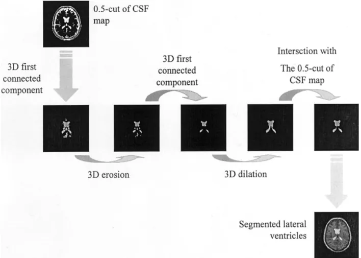
Extraction of LVs was processed from the CSF fuzzy map using simple mathematical morphology opera-tions (26). Under the hypothesis that LVs were the first 3D-connected components in the CSF fuzzy map, we applied the following transformations to this map to retrieve the LVs:
1. Computation of a slice where the LVs are visible. To achieve this, we noted that the slice maximizing the brain/background volume ratio always
con-tained a trace of the LV. We thus automatically processed the slice maximizing this ratio.
2. Determination of a voxel v included in the LV. Such a voxel is always located close to the middle of the slice of interest previously computed, with a very high membershipCSF(v) to CSF.
3. Search of the first 3D-connected component, in-cluding v in a binary 0.5 cut of the CSF map, obtained by retaining only voxels having a mem-bership to CSF at least equal to 0.5. The 0.5 cut was chosen because it theoretically minimized the error between the computed binary map and the “true” map represented byCSF.
4. 3D erosion of the resulting image, using a spheri-cal structuring element e of radius 1.5 mm, so as to select only the surest points of the first 3D-connected component. The value 1.5 mm was cho-sen to deeply dig into the binary structures and thus suppressed some small structures having a high membership to CSF and being detected in the previous step (e.g., sulci).
5. Search of the first 3D-connected component in the eroded image, in order to suppress small struc-tures (e.g., aqueduct of Sylvius).
6. 3D dilation of this latter image with the same structuring element e.
7. Intersection of the resulting image with the binary 0.5 cut of the CSF map, to overcome the possibly too important 3D dilation.
The resulting structure was considered to be the LVs. Figure 1 summarizes the whole set of operations.
Correction of Partial Volume Effects
Partial volume effects refer to when more than one tis-sue type occupies a single-voxel element, mainly at tissue boundaries. When considering the segmentation of the LVs, this effect is very pronounced on the edges of these structures, where a large group of voxels is actu-ally a mixture of WM and CSF (e.g., at the interface between ventricles and corpus callosum) (Fig. 2). As such, their gray levels are a mixture of WM and CSF ones, e.g., and lie in the range of GM gray levels in T1-weighted images. Several authors reported this fact as an error in brain tissue classification (9 –27), and Wang and Doddrell (28) showed that the ventricular volume could be underestimated by up to 30% if this error is not corrected. We propose here a fully auto-mated method to correct this partial volume effect.
For each voxel v, we computed the fuzzy member-ships to the set that “belongs to the partial volume effects” using concepts derived from data fusion (29). More precisely, we computed a partial volume effects fuzzy map MPVE (i.e., a distribution of possibilityPVE)
with
MPVE共v兲 ⫽ Min关共MWM䊝 f兲共v兲, 共MCSF䊝 f兲共v兲, MGM共v兲兴,
where f was a spherical structuring element of a 1-mm radius (we indeed estimated that partial volume effects could roughly occur in a 2-mm band around the ven-tricles). The minimum of memberships between (MWM䊝
f)(v), (MCSF 䊝 f)(v), and MGM(v) indeed represented the
possible areas of overlapping (and thus partial volume effects) between WM and CSF, counted as GM. The use of the minimum operator for the computation of partial volume effects refers to as a classical T-norm in fuzzy logic, generalizing the notion of intersection to fuzzy sets. Only the surest information is thus here retained: if one of the three memberships was null, e.g., if v didn’t belong to the fuzzy map MCSF 䊝 f, then v was not
considered to participate with partial volume effects. On the contrary, the three memberships had to agree
and to be equal to one to ensure that v fully participated with partial volume effects.
Voxels v of MPVEwith positive memberships were then
reclassified either as WM or CSF, depending on MWM
and MCSF maps: if the membership of v to CSF (i.e.,
MCSF(v)) was greater than its membership to WM
MWM(v), then v was reclassified as CSF; otherwise v was
reclassified as a WM voxel. We based this heuristic on the fact that degrees of memberships could be consid-ered as percentages of pure tissues in voxels (23).
Finally, the GM map computed with the fuzzy seg-mentation algorithm described in reference 23 could be corrected by subtracting the memberships of MPVEfrom
those of MGM, thus improving the fuzzy segmentation of
this tissue class.
RESULTS
Validation on a Brain Phantom
The extraction of tissue classes was validated by Barra and Boire (23) by using a computerized brain phantom developed at the McConnell Brain Imaging Center (24). We thus used SET1 images in this evaluation step. LVs were manually segmented by an expert from the high-resolution 1⫻ 1 ⫻ 1-mm T1-weighted image and rep-resented what we called the reference LVs in the follow-ing.
Complete extraction of LVs using mathematical mor-phology operations and corrections of partial volume
Figure 1. Extraction of the LVs.
effects was assessed by comparing the reference struc-tures with automatic segmented ones, computed from images MR1, MR2, and MR3. To achieve this compari-son, we used two numerical indexes: the first one was a similarity index, computed from the relative error in volume estimation when considering that the true vol-ume was given by the reference. If VT(VC, respectively)
was the true (computed, respectively) volume of the segmented LVs, this index was defined by
I1⫽ 1 ⫺兩VT⫺ VC兩 VT
I1 was as close to 1 as the volume assessment was correct.
The second one was a mean distance (in mm) of the computed lateral structure to the reference one, defined as: I2⫽
冘
PC僆 SC Min PT僆 ST 储PCPT储 Card共SC兲 ,where 储 䡠 储 denoted the Euclidean norm and PC (PT,
respectively) was a generic point of structure SC
(respec-tively ST).
These indexes allowed us to assess both the accuracy of volume estimation and the closeness of the
bound-aries of the structures (and thus the correction of par-tial volume effects). Table 1 summarizes the results of this comparison, and Figure 3 gives a 3D view of the ventricles, as well as an overlap of these structures on image MR2.
The true volume as estimated by the expert on the high-resolution MR image was 23.09 cm3. The volume
computed with our method was 22.99 (21.81 and 20.76, respectively) cm3on image MR1 (MR2 and MR3,
respectively), which led to I1 indexes of 0.99 (0.94 and 0.9, respectively). I1 indexes were very close to 1, indi-cating a good agreement between the computed LV vol-umes and the reference one, and indexes decreased as slice thickness increased because of stronger partial volume effects. Nevertheless, for image MR3, e.g., an I1 index of 0.90 revealed a 90% good estimation of the true volume. I2 indexes were small enough to be confident that boundaries between segmented LVs and reference ones were close enough.
To assess the contribution of partial volume voxels, we also compared the LV volumes with and without correction of partial volume effects. This implied the calculus of the relative difference ⌬V ⫽ 兩VC– V兩/V
be-tween the LV volume VCwith correction of partial
vol-ume effects and the LV volvol-ume V without correction. Table 2 shows the results for the three test images MR1,
Table 1
Comparison of Segmented Lateral Ventricles With Respect to a Reference
Slice thickness (mm) I1 (%) I2 (mm)
MR1 1 99.5 1.0
MR2 3 94.4 1.7
MR3 5 89.9 2.3
I1⫽ similarity index, I2 ⫽ boundaries distance.
Figure 3. 3D reconstruction of LVs and overlapping on an anatomic image. Table 2
Effect of the Partial Volume Effects Correction on Lateral Ventricles Volumes
Slice thickness (mm) VC(cm3) V (cm3) ⌬V (%)
MR1 1 22.99 20.92 9.6
MR2 3 21.81 18.64 14.5
MR3 5 20.76 16.44 20.8
VC⫽ volume with correction of partial volume effects, V ⫽ volume without correction of partial volume effects,⌬V ⫽ relative error in volume estimation.
MR2, and MR3, and Figure 4 shows the partial volume image computed from MPVE, the corrected GM fuzzy
map, and the reference one provided by the phantom on a slice of interest.
Volumes of LVs without correction were always lesser than those computed on corrected structures for about 15% for the three MR images. Results obtained on the thicker image MR3, where the partial volume effects were much more pronounced, showed that LVs were underestimated for about 25% with respect to corrected structures. These figures were in accordance with those published previously (28). The images of Figure 4 clearly show that partial volume effects were detected at the interfaces between CSF and WM, especially near the frontal and occipital horns (e.g., interface between the frontal horn and the corpus callosum). Moreover, the corrected GM map became very close to the reference one (we found (see reference 23) a mean Tanimoto index of 0.86 on MR1, MR2, and MR3 for the noncorrected GM map, and we found here a mean index of 0.92, revealing a higher similarity between the reference and the computed GM map).
Let us finally note that the method never failed to automatically segment LVs in about 20 seconds per volume.
Clinical Application
We propose to apply our method in the assessment of the enlargement of LVs on MR images of patients diag-nosed as potentially suffering from Alzheimer’s disease. The rate of total LV enlargement was indeed proved to be significantly different between Alzheimer’s patients and healthy controls, and it was more specific and sen-sitive to the diagnosis of the pathology than cross-sec-tional volumes at final evaluation (4). Moreover, Aral et al (30) and Creasey et al (31) proved that it was possible to differentiate Alzheimer’s patients from normal sub-jects by measuring ventricular size and the progressive enlargement of LVs. More generally, George, et al (32) proved that cognitive impairment and dilatation of ven-tricular size may be correlated.
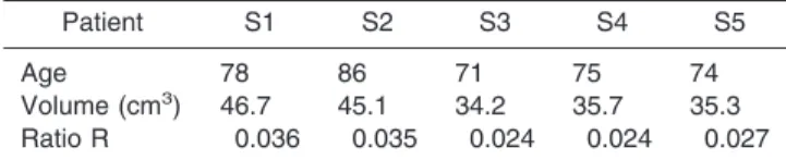
We used in this study the SET2 set of images, and we segmented the LVs for each subject, S1 through S5. LV volumes, as well as the ratio R ⫽ (LV volume)/(total brain volume), were computed for each patient, where the total brain volume was calculated from the tissue segmentation. Table 3 presents the results.
Aging has an effect on the increase of CSF volume in general and LV enlargement in particular, about 3 cm3
per year. Although we could not exactly discriminate
Figure 4. Partial volume and corrected GM fuzzy map on an MR slice of interest.
between the effects of age and pathology with our study, we could, nevertheless, compare our results with those of normal subjects of the same age. LV volumes of subjects S1 through S5 were larger (39.4⫾ 6 cm3; R⫽
0.029⫾ 0.005) than those published by Matsumae et al (33) (33 ⫾ 10 cm3; R⫽ 0.024 ⫾ 0.006) on 22 normal
subjects, aged 72⫾ 5, which might be an indication of the effects of the pathology.
Feasibility on Other MR Acquisitions
We finally propose to demonstrate that the method may be applied on several other classical MR acquisitions, represented by SET3. LVs were segmented by our method for subjects N1 through N4, and results were compared both intrasubject and with those of studies found in the literature.
Table 4 presents the results of the volumetric quan-tification. The ratio R ⫽ (LV volume)/(total brain vol-ume) was computed for each acquisition, where the total brain volume was calculated from the tissue seg-mentation. Volumes were consistent whatever the type of MR acquisition. Variation of the estimation of the volume, assessed by the maximum difference, for pa-tient N1 (N2, N3, and N4, respectively) was about 0.14 (0.05, 0.09, and 0.12, respectively) cm3. Ratios R were
homogeneous for each patient, from 0.010 (for N1) to 0.013 (for N3). For subjects comparable in age with our controls N1 through N4, results were comparable to volumes found in the literature. Puri, et al (34), e.g., found a ratio R of 0.011 ⫾ 0.3 and a LV volume of 15.3⫾ 4.18 cm3in a study of 12 controls, aged 27.92⫾
6.14. Matsumae, et al (33) found mean volumes of 17⫾ 5 cm3(and a ratio R of 0.013⫾ 0.03) on 12 subjects,
aged 35⫾ 6, and proved that their results agreed with already published data. Calmon, and Roberts (35) pro-cessed 18 images of a single healthy subject and found a mean volume of 14.9 ⫹ 0.1 cm3, with a Ratio R of
0.0092⫹ 0.1. Finally, Cramer, et al (36) found a mean LV of 17.4 cm3on 38 subjects of various ages with no
apparent pathology.
Since gray levels of GM are always located between those of CSF and white matter (MB) in the MR acquisi-tions of interest (gray levels are increasingly ordered LCS ⬍ GM ⬍ MB in T1-weighted images, MB⬍ GM ⬍
LCS in T2- and proton density-weighted images), the
fuzzy modeling MPVE of partial volume effects between
CSF and WM developed in the Correction of Partial Volume Effects section is always valid.
DISCUSSION
Since the in-slice resolution of our SET1 test images was at least 1 mm, we didn’t expect to have lesser values for I2 in the validation process. The highest I2 index (2.3 mm), and thus greatest errors in boundary estimations, was observed on an MR3 image near the frontal horn of the LVs. On the thicker slices, partial volume effects were indeed sensible, and maybe a fine layer of voxels weren’t counted as LVs, thus increasing the distance between the segmented edges and the true ones.
The use of fuzzy memberships allowed us to take into account ambiguities in the areas of partial volume ef-fects. Fuzzy logic proved its efficiency not only in the tissue segmentation step (23), but also in the modeling of partial volume effects. Degrees of memberships as computed by the possibilistic clustering algorithm de-veloped in our laboratory could indeed be considered as percentages of pure tissues in voxels, and the proce-dure of reclassification of ambiguous voxels takes this modeling into account.
The description of the structuring element f in the process, as proposed in this article, allowed the method to process almost the same results, whatever the slice thickness. The use of a metric description for f, as opposed to a classical voxel description, indeed allowed the algorithm to be independent from the specificity of the MR acquisition system (and in particular from the thickness of the slices). We now plan to process a fur-ther validation of this method by including a computa-tion of these indexes for several trained specialists, in order to manage the interoperator variability.
Let us finally note that the method we propose also allows the assessment of the longitudinal changes of full CSF volumes. It requires only the computation of the volumes on CSF maps computed with (23) and corrected with the method proposed in this article (i.e., without the segmentation of LVs). These volumes are useful for the study of not only Alzheimer’s disease, but also other pathologies and damages, such as hydro-cephalus or traumatic brain injury.
Table 3
Quantification of Lateral Ventricles Volumes on Alzheimer’s Patients
Patient S1 S2 S3 S4 S5
Age 78 86 71 75 74
Volume (cm3) 46.7 45.1 34.2 35.7 35.3
Ratio R 0.036 0.035 0.024 0.024 0.027
R⫽ (Lateral ventricles volume)/(total brain volume).
Table 4
Quantification of Lateral Ventricles Volumes on Different MR Acquisitions
Volume (cm3) R (⫻100) Patient N1 N2 N3 N4 N1 N2 N3 N4 Age 21 25 28 28 21 25 28 28 Volume (cm3) from T1 14.98 15.08 16.22 15.82 1.10 1.28 1.29 1.23 T2 15.12 15.13 16.13 15.68 1.11 1.29 1.29 1.22 Proton density 15.01 15.13 16.19 15.80 1.10 1.29 1.29 1.23
Ni⫽ normal subjects, R ⫽ (Lateral ventricles volume)/(total brain volume).
CONCLUSIONS
The method we proposed here to extract LVs from MR images was based on three steps: a preliminary step, which is a validated algorithm of tissue segmentation, and two new developments allowing both the automatic extraction of LVs and the correction of partial volume effects on their boundaries. The use of fuzzy member-ships throughout the algorithm allowed the manage-ment of uncertainty and imprecision inherent to MR data. In particular, it allowed consideration of partial volume effects as a problem of pure tissues blending, modeling degrees of memberships as mixture coeffi-cients. The segmentation of LVs with the management of partial volume effects was validated on a brain phan-tom and proved its efficiency. We then propose several potential applications, and we particularly focused on one of them concerning Alzheimer’s disease. We finally demonstrated its relative genericness by extracting LVs from several classical MR images and by assessing changes in volume quantification with respect to the acquisition type.
REFERENCES
1. Agartz I, Sa¨a¨f J, Wahlund L, Wetterberg L. Quantitative estimations of cerebrospinal fluid spaces and brain regions in healthy controls using computer-assisted tissue classification of MR images: rela-tion to age and sex. Magn Reson Imaging 1992;10:217–226. 2. Foundas AL, Zipin D, Browning CA. Age-related changes of the
insular cortex and lateral ventricles: conventional MRI volumetric measures. J Neuroimaging 1998;8:216 –221.
3. Kinoshita Y, Okudera T, Tsuru E, Yokota A. Volumetric analysis of the germinal matrix and lateral ventricles performed using MR images of postmortem fetuses. AJNR Am J Neuroradiol 2001;22: 382–388.
4. DeCarli C, Haxby JV, Gillette JA. Longitudinal changes in lateral ventricular volume in patients with dementia of the Alzheimer type. Neurology 1992;42:2029 –2036.
5. Murphy DG, DeCarli CD, Daly E, et al. Volumetric magnetic reso-nance imaging in men with dementia of the Alzheimer type: corre-lations with disease severity. Biol Psychiatry 1993;34:612– 621. 6. Andreasen NC, Swayze VW, Flaum M, Yates WR, Arndt S,
Mc-Chesney C. Ventricular enlargement in schizophrenia evaluated with computed tomographic scanning: effects of gender, age, and stage of illness. Arch Gen Psychiatry 1990;47:1008 –1015. 7. Shenton ME, Kikinis R, McCarley RW, Metcalf D, Tieman J, Jolesz
FA. Application of automated MRI volumetric measurement tech-niques to the ventricular system in schizophrenics and normal controls. Schizophr Res 1991;5:103–113.
8. Roy PD, Zipursky RB, Saint-Cyr JA, Bury A, Langevin R, Seeman MV. Temporal horn enlargement is present in schizophrenia and bipolar disorder. Biol Psychiatry 1998;44:418 – 422.
9. Brandt M, Bohan T, Kramer L, Fletcher J. Estimation of CSF, white and gray matter volumes in hydrocephalic children using fuzzy clustering of MR images. Comput Med Imaging Graph 1994;18:25– 34.
10. Tsunoda A, Mitsuoka H, Sato K, Kanayama S. A quantitative index of intracranial cerebrospinal fluid distribution in normal pressure hydrocephalus using an MRI-based processing technique. Neuro-radiology 2000;42:424 – 429.
11. Luks TL, Goodkin DE, Nelson SJ, et al. A longitudinal study of ventricular volume in early relapsing-remitting multiple sclerosis. Multiple Sclerosis 2000;6:332–337.
12. Paravision™, version 1.0. Karlsruhe, Germany: Brucker Medizin-technik, GmbH, 1996.
13. Chuang CH, Lie WN, Peng WH. Lateral ventricle boundary segmen-tation and features measurement in CT brain images. Proceedings of the Annual Fall Meeting of the Biomedical Engineering Society, Washington, WA, 2000.
14. Robb RA. A software system for interactive and quantitative anal-ysis of biomedical images in 3D imaging in medicine. In: Hohne K, Fuchs H, Pizer S, editors. NATO ASI series. New York: Springer Verlag; 1990. p F60.
15. Johnson LA, Pearlman JD, Miller CA, Young TI, Thulborn KR. MR quantification of cerebral ventricular volume using a semi-auto-mated algorithm. AJNR Am J Neuroradiol 1993;14:1373–1378. 16. Worth AJ, Makris N, Patti MR, et al. Precise segmentation of the
lateral ventricles and caudate nucleus in MR brain images using anatomically driven histograms. IEEE Trans Med Imaging 1998; 17:303–310.
17. Collins DL, Kabani NJ, Evans AC. Automatic volume estimation of gross cerebral structures (Abstract 0702). In: Proceedings of Hu-man Brain Mapping, Montreal, Canada 1998.
18. Ferrant M, Cuisenaire O, Macq B. Multi-object segmentation of brain structures in 3D MRI using a computerized atlas. SPIE Med Imaging 1999;3661:986 –995.
19. Musse O, Bueno G, Heitz F, et al. Hybrid atlas-based and image-based approach for the automatic segmentation of brain struc-tures. In: Proceedings of the 8th Annual Meeting of ISMRM, Denver, 2000. p 804.
20. Undrill PE, Delibasis K, Cameron GG. Application of genetic algo-rithms to geometric model-guided interpretation of brain anatomy. Pattern Recognition 1997;30:217–227.
21. Duta N, Sonka M. Segmentation and interpretation of MR brain images: an improved active shape model. IEEE Trans Med Imaging 1998;17:1049 –1062.
22. Philipps WE, Velthuizen RP, Phuphanich S, Hall LO, Clarke LP, Silbiger ML. Application of fuzzy C-means algorithm segmentation technique for tissue differentiation in MR images of a hemorragic glioblastoma multiforme. Magn Reson Imaging 1995;13:277–290. 23. Barra V, Boire JY. Tissue characterization on MR images by a possibilistic clustering on a 3D wavelet representation. J Magn Reson Imaging 2000;11:267–278.
24. Kwan R, Evans A, Pike B. An extensible MRI simulator for post-processing evaluation. In: Proceedings of the Visualization in Bio-medical Computing Conference (VBC 1996). Lecture notes in com-puter sciences, vol. 1131. Springer Verlag; 1996. Hamburg, Germany. p 135–140.
25. Haase A, Frahm J, Matthaei D, Ha¨nicke W, Merboldt KD. Rapid three-dimensional MR imaging using the FLASH technique. J Com-put Assist Tomogr 1986;10:363–368.
26. Serra J. Image analysis and mathematical morphology. Academic Press; London, 1982. p 610.
27. Reiss A, Hennessay J, Rubin M, et al. Reliability and validity of an algorithm for fuzzy tissue segmentation of MRI. J Comput Assist Tomogr 1998;22:471– 479.
28. Wang D, Doddrell DM. A segmentation-based and partial-volume compensated method for an accurate measurement of lateral ven-tricular volumes on T1-weighted magnetic resonance images. Magn Res Imaging 2001;19:267–272.
29. Bloch I. Information combination operators for data fusion: a com-parative review with classification. IEEE Trans Sys Man Cybernet-ics 1996;1:52– 67.
30. Aral H, Kobayashi K, Ikeda K, et al. A computed tomography study of Alzheimer’s disease. J Neurol 1983;229:69 –77.
31. Creasey H, Schwartz M, Frederickson H, Haxby JV, Rapoport SI. Quantitative computed tomography in dementia of the Alzheimer’s type. Neurology 1986;36:1563–1568.
32. George AE, de Leon MJ, Rosenbloom S, et al. Ventricular volume and cognitive deficit: a computed tomographic study. Radiology 1983;149:493– 498.
33. Matsumae M, Kikinis R, Mo´rocz I, et al. Age-related changes in intracranial compartment volumes in normal adults assessed by magnetic resonance imaging. J Neurosurg 1996;84:982–999. 34. Puri BK, Hutton SB, Saeed N, et al. A serial longitudinal
quantita-tive MRI study of cerebral changes in first-episode schizophrenia using image segmentation and subvoxel registration. Psychiatry Res 2001;106:141–150.
35. Calmon G, Roberts N. Automatic measurement of changes in brain volume on consecutive 3D MR images by segmentation propaga-tion. Magn Res Imaging 2000;18:439 – 453.
36. Cramer GD, Allen DJ, DiDio LJ, Potvin W, Brinker R. Evaluation of encephalic ventricular volume from the magnetic resonance imag-ing scans of thirty-eight human subjects. Surg Radiol Anat 1990; 12:287–290.