Axisymmetric modes in hydromagnetic waveguide.

Lr

AXISYMMETRIC MODES IN

YDROMAGNETIC WAVEGUIDE

GERALD B. KLIMAN

Le

TECHNICAL REPORT 449

FEBRUARY 28, 1967

MASSACHUSETTS INSTITUTE OF TECHNOLOGY

RESEARCH LABORATORY OF ELECTRONICS

CAMBRIDGE, MASSACHUSETTS

QCUMENT OFFICE

a

T

BOO

36-j

RE5EARCH LABORATORY OF ELECTRONCt-MASSACHUSTTS INST!tUTE OF TtECtNQ6O0

CMi IDE. MASSACHUSETTS 021)9, U,,SA,

~-~ ~-~~-`---..

The Research Laboratory of Electronics is an interdepartmental laboratory in which faculty members and graduate students from

numerous academic departments conduct research.

The research reported in this document was made possible in part by support extended the Massachusetts Institute of Tech-nology, Research Laboratory of Electronics, by the JOINT SER-VICES ELECTRONICS PROGRAMS (U.S. Army, U.S. Navy, and U.S. Air Force) under Contract No. DA36-039-AMC-03200 (E); additional support was received from the National Science Foun-dation (Grant GK-524).

Reproduction in whole or in part is permitted for any purpose of the United States Government.

MASSACHUSETTS INSTITUTE OF TECHNOLOGY

RESEARCH LABORATORY OF ELECTRONICS

Technical Report 449 February 28, 1967

AXISYMMETRIC MODES IN HYDROMAGNETIC WAVEGUIDE

Gerald B. Kliman

Submitted to the Department of Electrical Engineering, M. I. T., May 28, 1965, in partial fulfillment of the requirements for the degree of Doctor of Science.

(Manuscript received November 1, 1965)

Abstract

The axisymmetric, transverse magnetic field modes of a hydromagnetic or Alfven waveguide are studied experimentally and theoretically. An experiment was performed to examine with precision measurements the steady-state half-wave resonances of a short section of hydromagnetic waveguide with a liquid metal (NaK) used as the fluid conductor. The response to a step of current was also examined. The theory of uni-form hydromagnetic waveguides is reviewed and extended by reconsideration of the propagation constant and theories for the effects of transverse fields, viscosity, finite conductivity walls, and bulk motion. A theory predicting the effects of nonuniform density or magnetic field is developed and verified in the experiment.

TABLE OF CONTENTS

Glossary v

I. INTRODUCTION 1

1. 1 Orientation 1

1.2 Previous Experiments 1

1.3 Review of Theoretical Papers 3

1.4 Organization of the Report 5

II. THEORETICAL FOUNDATIONS OF THE EXPERIMENT 7

2. 1 Propagation Constant 7

2. 2 Lossy Hydromagnetic Resonator 17

2.3 Nonuniform Media 22

III. EXPERIMENT 27

3. 1 Description of the Apparatus 27

3. 1. 1 The Resonator 27 3. 1.2 Electronic Systems 29 3. 1. 3 Magnetic Field 32 3.2 Experimental Procedures 34 3. 2. 1 Resonance Measurements 34 3.2.2 Step Response 34 3. 2. 3 Field Measurements 34 3.3 Summary of Results 35

IV. ANALYSIS OF THE RESULTS 39

4. 1 Comparison of Experiment and Theory 39

4. 1. 1 Step Response 39

4. 1.2 Resonance 40

4.2 Comparison of Uniform and Nonuniform Field Results 43

V. CONCLUSIONS AND RECOMMENDATIONS 48

5. 1 Experiment 48

5. 2 Theory of Uniform Hydromagnetic Waveguides 48

5.3 Nonuniform Media 49

5.4 Recommendations for Further Research 50

5. 4. 1 Experiment 50

5.4.2 Theory 50

CONTENTS APPENDIX A APPENDIX B APPENDIX C APPENDIX D APPENDIX E APPENDIX F APPENDIX G APPENDIX H APPENDIX I APPENDIX J APPENDIX K APPENDIX L

Effects of Usually Neglected Factors

Nonuniform Density and the Perturbation Expansion

Inhomogeneous Magnetic Field

Hydromagnetic Columns

Alternate Derivation for Axisymmetric TM Modes in a Uniform Waveguide

Resonator Design Electronic Systems

Design of the Nonuniform Field

NaK Handling Techniques

Algebraic Details of the Perturbation Solution

Hydromagnetic Capacitor Hydromagnetic Resonators Acknowledgment References iv 52 58 70 79 82 83 86 87 89 90 92 94 97 98

GLOSSARY Symbol Definition p Density V, v Velocity P, p Pressure J, j Current density B, b Magnetic field Conductivity E, e Electric field

Vo Magnetic susceptibility of free space

w Radian frequency

K, k Propagation constant

a Bessel function root

C,c Alfven speed a Waveguide radius b Wall thickness g Exciter radius i f Frequency I Circuit current T Mode factor 1 Magnetic diffusivity y Mode factor 2 Resonator length J _n Bessel function d Expansion parameter x Normalized radius v Viscous diffusivity Absolute viscosity v

GLOSSARY Symbol Definition CHM Hydromagnetic capacitance Vector field A Vector field Scalar potential vi

I. INTRODUCTION 1. 1 ORIENTATION

When a fluid is allowed to have electrical conductivity and magnetic fields are applied, a wide range of new and varied phenomena arise.1 Among the most important of these is the possibility of a magnetohydrodynamic wave in which stored energy is exchanged between the wave magnetic field and the kinetic energy of motion in the fluid. Such waves were predicted by Alfvdn,Z in 1942, but were not actually observed3 until 1954. These waves, now known as Alfvdn waves, are of importance in the entire range of magnetohydrodynamic phenomena from power generation and thermonuclear fusion through microwave devices to the operation of the solar system and the galaxy.

In view of the importance of Alfven waves, it is not surprising that there have been many theoretical studies of this phenomenon and its role in other processes. Experi-mental studies, however, have been few and more in the nature of demonstrations

showing that an Alfv6n type wave existed, rather than in the nature of a precise verifi-cation of the wave properties.

This study was undertaken in an attempt to perform an experiment of sufficient pre-cision and accuracy to prove unequivocally the theory of Alfvdn waves in detail and justify the assumptions upon which it is based. Since such experiments must be per-formed in a laboratory, they become studies of the Alfven or hydromagnetic waveguide. Liquid metal was chosen as the fluid conductor in order to eliminate the bothersome and poorly understood properties of suitable plasmas so that only the magnetohydrodynamic interaction would be of importance.

During the design of the experiment, it became evident that there were some gaps in the theory of hydromagnetic waveguides, such as lack of theoretical developments and incomplete or inconvenient interpretations of existing theory. Therefore, theoretical studies were also undertaken in an effort to understand more fully the properties of hydromagnetic waveguides.

1.2 PREVIOUS EXPERIMENTS

There had been eight experiments to observe Alfven waves in the laboratory before the present study was undertaken. A comparison of these experiments is presented in Section II. The experiments will be described in chronological order.

The first attempt to observe an Alfv6n wave was made in Alfven's laboratory in Sweden by S. Lundquist,4 in 1949. His experiment consisted of a circular cylinder, its interior insulated, placed with its axis vertical and parallel to the magnetic field in which it was immersed. The conducting fluid was mercury. A finned disk was placed at the bottom of the cylinder and excited in torsional vibrations by a shaft brought through the bottom of the cylinder. Waves transmitted to the free surface near the top of the cylinder were observed by the motion of a small mirror floating there. This experiment

did not succeed in demonstrating Alfv6n waves. It was thought that turbulence caused by the fins on the exciting disk was responsible, but it is shown in Section II that no Alfven wave could exist in mercury at the magnetic field strength used.

The second experiment was done by B. Lehnert,3 in 1954, also in Alfven's labora-tory. This experiment was quite similar to Lundquist's except that heated sodium was used as the fluid conductor, an electric field probe was used at the free surface in place of the mirror, and excitation was by means of a copper disk suspended on a coaxial shaft (also insulated). Except for the copper disk that was used to eliminate the supposed turbulence problem, all changes were made in order to contain the highly reactive liquid sodium under an inert atmosphere. This experiment succeeded in demonstrating the existence of an Alfven wave, but with considerable discrepancy between experimental results and theory.

In 1961, two experiments were conducted in England and in the United States, in both of which transient plasmas were used as the fluid conductor. In the experiments of Wilcox, da Silva, Cooper and Boley, at the Lawrence Radiation Laboratory, a copper cylinder, insulated at both ends and filled with hydrogen gas, was immersed in a mag-netic field parallel to its axis. A cylindrical copper plug electrode was set coaxially into one of the end insulators. A capacitor bank was discharged from the coaxial electrode to the walls, thereby initiating a shock that propagated to the other end of the cylinder and left a region of decaying ionized hydrogen behind it. When the shock reached the end of the cylinder, the capacitor bank was short-circuited, and a short time later another capacitor bank was discharged from the coaxial electrode to the wall through the ionized gas. The capacitor bank was allowed to ring at a frequency below the ion-cyclotron resonance. The transit time of the waves that were generated was then meas-ured. This experiment succeeded in demonstrating more of the qualitative properties of Alfven waves, but uncertainties in the effective plasma density and conductivity pre-vented precise conclusions.

The experiments of Jephcott, Stocker, and Woods,6 at the Culham Laboratory, were similar. In this case, the magnetic field coils were excited by a third capacitor bank, the cylinder was made of quartz, except for a narrow conducting ring near the excitation electrode, and the plasma was generated by a longitudinal arc. Again, Alfvdn waves were observed, but precise comparisons with the theory could not be made, because of uncer-tainties of the magnetic field and the effective density. In both experiments, transit-time measurements were made from oscilloscope photographs of a single transient.

A series of experiments was carried out, in 1961, by Nagao and Sato,3 2 at Tohoku University. The general arrangement, magnetic field, ionization, and excitation were almost identical to those of Jephcott, Stocker, and Woods.6 The precision of their

results was much poorer, but they also investigated the reflection of hydromagnetic waves from an abrupt change of magnetic field.

In 1962, experiments aimed at an investigation of the "Luxembourg effect" (inter-modulation of radio waves in the ionosphere caused by motion of the ions) was initiated

at the Air Force Cambridge Research Laboratories by DeCourcy and Bruce. They hoped to observe this effect, in the laboratory, by the coupling of Alfven waves to elec-tromagnetic waves. Their experimental apparatus was built of two coaxial quartz tubes

sealed at the ends. The inner walls of the annulus were lined with copper screen in order to support both Alfv~n and electromagnetic TEM modes. The inner cylinder contained a powerful ultraviolet source to ionize cesium vapor in the annulus by radiation. No results have been reported at this time.

Another series of experiments was carried out at the Massachusetts Institute of Technology, in which sodium-potassium eutectic alloy (78% potassium, 22% sodium), known as NaK, was used as the fluid conductor. The first set of experiments was done by N. Gothard,8 in 1962. His apparatus consisted of a cylindrical tank, closed at both ends, constructed entirely of stainless steel and filled with NaK. Excitation was by means of a copper disk, insulated except for the edge, mounted on a cantilever some distance from one end of the cylinder. Waves were detected by a magnetic pickup coil mounted on a cantilever that could be traversed in both radius and height. This experi-ment again demonstrated the existence of Alfvdn waves, but no attempt at precision measurements was made. In fact, many of the results were later shown to be of doubtful value, because of a lack of axisymmetry in the excitation and various mechanical vibra-tions induced in the detector by the motion of the cantilevered exciter.9Additional experi-ments were run at a later data in the same apparatus by Jackson and Carson. 1 0Drastic modifications of this apparatus were made by Wessler, Jackson, and Kliman1 1 to utilize the TEM modes for an educational film on Magnetohydrodynamics.

A series of steady-state experiments was carried out by P. Jameson, 12

in 1963, at Cambridge University. The apparatus consisted of two coaxial cylinders sealed at either end to form a closed annulus constructed entirely of stainless steel. A toroidal coil was wound on this structure, threading the core, as if it were an inductor with a liquid-metal core. The fluid conductor was heated sodium. The coil was excited with a current, which caused current sheets to form at each end, propagate out, and reflect from the other end. A magnetic pickup coil was used to detect the waveforms of the magnetic fields. The results of this experiment demonstrated Alfven waves more precisely than previous work, but again without the precision attainable in steady-state resonance measurements.

1.3 REVIEW OF THEORETICAL PAPERS

The number of papers on hydromagnetic waves is voluminous (see, for instance, Ramer or Clauser4 ). Only a few of the more pertinent papers will be mentioned here. One of the many treatments of waves in a compressible medium with an applied uniform steady magnetic field is that of Banos.15

The first treatment of a hydromagnetic waveguide was performed by Lundquist4 in connection with his experiment. Essentially, he developed the behavior of the lowest axisymmetric transverse magnetic (TM) mode in a cylindrical waveguide. This theory

was later considerably improved by Lehnert, who extended consideration to the entire set of axisymmetric TM modes in a coaxial structure, and took into account the finite size of his experimental apparatus and the exciter. Blue1 6 attempted to explain the dis-crepancies of Lehnert's experiment, by considering the effect of viscosity in an exact manner, and found that it did not significantly affect the results.

Newcomb,17 in 1957, first noted the similarities between hydromagnetic and elec-tromagnetic waveguides. In a limited way, he examined the TM, TE, and TEM modes in waveguides filled with perfectly conducting fluid. Finite conductivity, compressibility, and ion-cyclotron effects were included as perturbations. Perfectly conducting wave-guides were put on a firmer basis by Gajewski,18 in 1959. This study included com-pressibility and considered both rigid and flexible walls. Soon thereafter, Shmoys and Mishkin9 examined the same area, but from a different point of view. They considered the hydromagnetic waveguide as if it were an electromagnetic waveguide characterized by a dielectric tensor. Gould2 0 considered the various modes in a cylindrical wave-guide, and included a discussion of how modes could be excited. In 1961, Woods2 1 made the most thorough and inclusive analysis, thus far, of the cylindrical hydromagnetic waveguide, in connection with the Culham Laboratory experiments.6 This analysis included anisotropic conductivity, pressure and viscosity, ion-cyclotron resonance and the presence of ions, neutrals, and electrons. Aspects of hydromagnetic waveguides were studied by Rook, in connection with his work on surface waves, from a somewhat more general point of view for a simple medium.

Hydromagnetic resonators were considered, in 1960, by Gajewski and Mawardi.Z3 In this study, the fluid was a perfect conductor and the terminations either perfect con-ductors or insulators. In 1962, Rink2 4 extended the theory of hydromagnetic resonators by including finite fluid conductivity and lossy reactive terminations. What was more important, he found the electrical input impedance of the resonator for a practical excitation structure, thereby allowing consideration of lumped terminations.

Nonuniform density or magnetic field problems have been considered primarily in connection with cosmic or ionospheric studies.1 ' _, 1 3_,1 4 _{There has been, however, only}

one study of nonuniform density in a laboratory situation.2 5 _{On the other hand, there}

has been a great deal of interest in lossless nonuniform electromagnetic waveguides and resonators (see, for instance, Berk 26).

In 1961, Gajewski and Winterberg2 7 '28 made a thorough study of Alfven waves in axisymmetric nonuniform magnetic fields, and in an unbounded incompressible medium of infinite conductivity. They showed that an Alfv6n wave is always possible, as are other types of waves which do not exist in a uniform field. Their interest was primarily in the reflection of Alfven waves, such as those in a magnetic mirror.

Pneuman25 has analyzed what is essentially a cylindrical hydromagnetic wave-guide with insulating walls and radial variation of density. His analysis was based on the assumption of infinite conductivity, leading to a nonuniform phase front after the wave had been launched from one end of the guide. Finite conductivity

was then included as a perturbation on this solution. It is shown in the present study, however, that the addition of finite conductivity allows the propagation of a plane wave front that responds to average, rather than local, properties of the medium.

1.4 ORGANIZATION OF THE REPORT

Section II lays the theoretical foundations of the experiment that forms the base of this work. Prior theoretical and experimental work on unterminated

hydro-magnetic waveguides is reviewed. New interpretations are placed on the

dimen-sionless groups appearing in the propagation constant, which lead to a simple and convenient way of depicting its behavior. New results on the effects of vis-cosity, finite-conductivity walls, and transverse-field components are obtained (see

also Appendix A). The response of a hydromagnetic resonator to steady-state

sinusoids and suddenly applied steps of current is described. An equivalent

cir-cuit for the resonator near resonance is developed (see also Appendix L). The

effect of bulk motion of the fluid on the steady state and step response is also

considered (see also Appendix K). The response is found to consist of a damped

sinusoid, because of the multiply reflected Alfven wave superimposed on a ramp, resulting from the "motoring" of the fluid acting as a capacitance. A theory for

nonuniform media is developed. A radially nonuniform density is considered (see

also Appendix A), as well as a nonuniform but axisymmetric magnetic field. It

is shown that, if the magnetic field does not vary too strongly, this case may

be reduced to that of variable density (see also Appendix C). A perturbation

theory is developed to solve the resulting equations. The expansion for the prop-agation constant obtained by this method indicates that the nonuniform hydromag-netic waveguide responds as if it were a uniform waveguide having averaged properties

(see also Appendix B).

In Section III the experimental apparatus, procedures, and results are described. The apparatus may be divided into three groups: the resonator, which was specially constructed to conform as closely as possible to the theorectical model and to be safely and conveniently used with NaK (see also Appendix F); the electronic systems for exciting the resonator and measuring both steady-state resonance and step response (see also Appendix G); and the magnetic field. Two field configurations were used, one uniform and the other conforming to the relatively simple variation on which the non-uniform field theory was based (see also Appendix H). The experimental procedures were primarily developed to achieve maximum field strength and precision in the oper-ation of the magnet. Care was taken to eliminate extraneous signals and to achieve max-imum precision in all measurements. The principal results of the experiments are summarized.

Section IV presents an analysis of the experimental data and compares the results with theory. The resonator behavior is shown to conform closely to the performance

predicted by small-signal Alfv6n wave theory in both the step and steady-state responses. A comparison of behavior in uniform and nonuniform fields confirmed the theory devel-oped in Section II; however, the precision was not sufficient to draw firm conclusions about which type of average was more correct.

Section V summarizes the present work and gives recommendations for further research.

II. THEORETICAL FOUNDATIONS OF THE EXPERIMENT

The propagation constant for a uniform hydromagnetic waveguide with finite con-ductivity will be studied first. Consideration of some nonideal properties such as vis-cosity, finite-conductivity walls, and transverse fields will be considered. The response of a hydromagnetic resonator under various kinds of excitation will then be examined.

Finally, the effect of the Alfven velocity varying as a function of radius will be studied. 2.1 PROPAGATION CONSTANT

Several investigators have examined the uniform hydromagnetic waveguide in some detail. Their analyses have included almost every possible effect that one could imagine to occur when the medium is plasma or liquid. The most general case, however, tends to obscure rather than illuminate the relevant issues. Experimental investigations have

also been made indicating that the basic phenomena in the hydromagnetic waveguide may be explained by only a few of the possible physical processes taking place in a plasma or by rather gross averages of the microscopic phenomena in a plasma.

In this investigation, attention is fixed primarily on an experiment in which a liquid metal is used as the fluid conductor. Thus most of the bothersome properties of plasmas

are eliminated from consideration. The remaining properties of interest are density, electrical conductivity, viscosity, and magnetic permeability. The electric permittivity is not important, because of the extremely low frequencies characterizing the Alfv6n wave. No attempt will be made to cover all factors in one single formulation. Instead, the "ideal" hydromagnetic waveguide, that is with only density, conductivity, and perme-ability considered, will be examined in some detail. Then the principal neglected effects of viscosity and fringing fields will be examined to show their effect on the "ideal" situation.

a. Finite Conductivity Waveguide

Wave equations -We shall now be concerned with the "ideal" hydromagnetic wave-guide. Consider a uniform hollow cylinder of arbitrary cross section as shown in

x

Fig. 1. Hydromagnetic waveguide.

z

Fig. 1. It is made of either perfectly conducting or perfectly insulating material, filled with a conducting fluid of density p and conductivity , and with its axis aligned with a

7

_______lllilliill___---.-.-.-uniform steady magnetic field Bo = i Bo The applicable laws are then Maxwell's equa-tions

V X E = a _at (1)

aE

X B = oJ + e at (2)

to which must be added the momentum equation and Ohm's law.

Dv - j -(

Dv = -Vp+ J X B(3)

Dt

J = 0r(E+vX B). (4)

These equations can be linearized in the usual way by letting each quantity vary as

= A _o+ aei o t, (5)

where la

|

V X e = -iob (6)

V X b = Oj (7)

iwpv = -Vp + X B (8)

j = -(e+v X Bo), (9)

where the displacement current term in Eq. 2 has been dropped through the assumption of low frequencies and high conductivity. For circular cylinder waveguides and trans-verse magnetic field modes Eqs. 6-9 may be reduced to a single equation in, for instance, b. (e i n variation is assumed.)

d[I rb +- - k2(o + b 0. (10)

dr r r

L

The resulting propagation constant is

2 FLP " + iol -2 = )oP , ) (11) k2 o c mn 2 2 B Br 1 + . lop

where a _mn is the mth root of the n th-order Bessel function and depends on the wall material (conducting or insulating), as well as on mode number. Equation 11 may be

8

rewritten in a simpler form as Z₁ (12) Z1 + i where B c - Alfv6n speed (13) 2 a

1 mn Lower critical frequency (14)

Za Loa B2a

2 2p * Upper critical frequency (15)

Propagation will take place only if

al< < W2' (16)

thereby dividing the range of possible frequencies into three regions. For << ol kmn approaches the asymptote

k _mn = _c 1 (l-i). (17) For w >> 2' k = (1-i). (18) mn c For w1 << <<( °2'

k

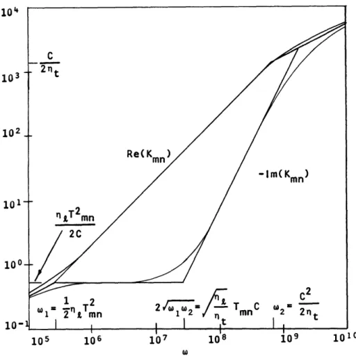
Equation 19 may also be looked upon as having two asymptotes in the imaginary part for relatively low and relatively high frequencies. These several asymptotes are plotted in Fig. 2. Note that their intersections occur at the critical frequencies. For com-parison, an exact evaluation of kmn for NaK is also plotted in Fig. 2.

Inspection of Fig. 2 reveals that in order for low-attenuation Alfven waves to exist, W2 >> W1; this, in turn, means high conductivity ar, high magnetic field Bo, small

den-sity p, large radius a, and small mode number a The last means that the lowest

mn

order or simplest modes must be excited and that a conducting, rather than an insulating, wall should be used. In each case, then, the modes having the smallest

9

10

101

100

10 102 103 104

Fig. 2. K -w diagram for a liquid metal (NaK). = 2. 63 X 10 Z/m; p = 8.5 X 10 kgm/m3 ; B = 0.8 w/m; a = 0. 19 m; first

axisym-metric mode; insulating wall.

attenuation are those with the simplest field configuration, that is, for rota-tional symmetry (n=0) and the smallest nonzero root of the Bessel function (m=l).

The lowest attenuation for all modes is in the TM10 mode in a perfectly con-ducting cylinder.

Equations 17 and 18 are characteristic of diffusion phenomena. At low frequencies the magnetic field diffuses through the fluid in a time that is short compared with the period of the excitation. Thus the field is not convected by the fluid. At high

fre-quencies the field cannot penetrate the fluid. Thus the fluid is not convected by the field. But if X satisfies condition (16), there is a region in which mutual convection of the

fluid and the field gives rise to the Alfv6n wave.

Notice that the lower limit of the Alfven region is controlled by conductivity and geometry, while the upper limit is controlled by conductivity, density, and applied field. The frequency below which, under condition (16), the waveguide is distortionless is twice the geometric mean of the upper and lower limits. Now,

- - Magnetic Reynolds number

1 T

mn

22 B2

= o Lundquist number

W CP

Thus, in order that an Alfvdn wave exist, both the magnetic Reynolds and Lundquist numbers must be large compared with unity.

Listed below in tabular form is a comparison of a number of Alfven wave experi-ments in terms of the critical frequencies.

Experimenter Medium fl f2

1. Jephcott, Stocker, arc plasma 46.5 kc 51. 3 Me

and Woods6

2. Wilcox, daSilva, shock plasma 41.4 kc 111.0 Mc

Cooper, and Boley5

3. DeCourcy and Bruce7 irradiated gas 0 (TEM) 4. 07 Mc

4. Gothard,8 and NaK 9.75 cps 158 cps

Jackson and Carson1 0

5. Lundquist4 Hg 159 cps 10. 3 cps

6. Lehnert3 Na 21.5 cps 770 cps

The solutions to the hydromagnetic wave equations have been examined in some detail by Rook,22 by utilizing vector potentials (Appendix D). He found that, in gen-eral, for an infinitely long cylinder of arbitrary cross section there are four possible solutions. One of these was identically zero, and a second was a potential flow in which the current density was identically zero and therefore not Alfven. The remaining solu-tions are Alfvdn, one consisting of a set of TE modes in which the perturbation elec-tric field is transverse to Bo, and the other a set of TM modes in which the perturbation

magnetic field is transverse to Bo.

If the waveguide is of a simple cross section such as a circle of radius a, the expressions for the various perturbation fields may be found closed form.

Quoting Rook, we have the expressions for the TM waves with all quantities

varying: A = a ei ( n O+ k z +wt ) (20) v CTM (1 + 4 )[r Jn(Tr) ir -TJn(Tr)i- (21) ikB b - MAv (22) 11 I- - - - ~111

kB J= CTM _(A4Looo e = -c TMikBo[ T_{TM k} (2 +k [T(Tr Trkn (T +kv)M AITJIn (Tr)lr 2 A n rT~r k2 A n rkr(1 Jn(Tr) i0 + Jn(Tr)iz k2 2) T / p = 0, where 2 A k2C2 B2 C2 - o 11oP -T 2 =k 2 + irp (23) Jn(Tr) i. - (1 -MA2 ) Jn(Tr) il (24) (25) (26) (27) °0 2) W6~~ (28)

and CTM is an arbitrary constant. The TE modes are

v = CTE ikJ n (Tr) + T Jn(Tr) ikB b = _c) MAv i0 + TJn(Tr) iz kB in J = +Te o (T +k )MA(t JnTr)r-J(Tr) i e=cTEik A n( Tr e = -Ci kB M - r Jn(Tr) iT r) T p = -cTEip ik Jn(Tr) The potential modes are

= C[ikJ (ikr) nJn(ikr) jr- 0+ ikJn(ikr) i]

kB_{0_}

J 0 v

j=0

e = - ikB[kr Jn(ikr) ir-Jn(ikr) 1ie

p cppJn(ikr)

]

Boundary conditions - The assumption of a rigid-wall cylinder means that the nor-mal component of velocity at the wall must be zero.

vr(a) = 0. (39)

Since viscosity has been neglected, there is no restriction on the tangential com-ponent of velocity. The effect of viscosity is considered in section 2. lb.

If the wall is assumed to consist of a perfectly conducting material (=oo), the tan-gential component of electric field at the wall must be zero.

ez(a) = ee(a) = . (40)

There is no restriction on the normal component, since a surface charge may exist on the interface. The tangential components of the magnetic field may be satisfied by

sur-face currents, but the normal component must be zero.

br(a) = 0. (41)

But since the perturbation magnetic and velocity fields are proportional, it is sufficient to require Eq. 39 only.

If the wall is assumed to consist of a perfectly insulating material (-=0), the nor-mal component of the current must be zero at the wall.

jr(a) = 0. (42)

There is no restriction on the tangential components of the electric field except continuity at the boundary; thus, there is a possibility of an external field structure. Again, as in the case of a perfectly conducting wall, the normal component of magnetic field will be zero if the normal component of velocity is zero. There is no restriction

other than continuity on the tangential components which allow for the existence of an external magnetic field.

The rigid walls will make up whatever pressure is required by the various modes, if they exist, so that boundary conditions on the pressure need not be considered further.

Single mode propagation - An examination of Eqs. 21-38 for the field quantities and boundary conditions (39) to (42) reveals that while all of the individual modes may prop-agate in a perfectly conducting cylinder, only the n = 0 modes may propprop-agate in a per-fectly insulated cylinder. The difficulty comes in attempting to satisfy simultaneously the conditions on normal current and velocity. This point has not been generally rec-ognized but was considered by Woods.2 1 The problem of a general disturbance on a perfectly flexible cylinder has also been considered by Rook.2 2

If attention is restricted to those modes that may propagate singly, the propagation constant may be considered in more detail. For the TM and TE modes, application of

the boundary conditions (39) and (40) for a perfectly conducting rigid cylinder of radius a yields:

13

Jn(Ta) = 0 TM modes (a all= ) (43)

n wall

Jn(Ta) = 0 TE modes (awall = 0o). (44)

For a perfectly insulating rigid cylinder of radius a, application of the boundary con-ditions (39) and (42) yields for the n = 0, TM and TE modes:

Jo(Ta) = 0 n = ; (wall =0). (45)

In each case, the boundary condition fixes the value of Ta and thus k. All modes except the TEmO mode in an insulated cylinder have their fields confined to the region r < a. Continuity of the tangential magnetic field requires an external field to match the 0 component in Eq. 29. If the mth root of the nth-order Bessel function or its

deriv-ative is denoted a mn, then

Ta = a . (46)

A mode factor Tmn similar to that used in ordinary waveguide theory would then be

a

T _mn mn _a (47)

Solving Eq. 28 for k2 then yields, as before, T2 + i 2 rQ mn mk - 2m(48) mn Tt 1 + c2 1+ icn t where 1 ,- t t o,tLO (49)

are the longitudinal and transverse magnetic diffusivities corresponding to a conductivity tensor of the form

0K:

°L

O -t (50)

0 0 'T

which results from a simpler derivation for the symmetric TM modes (Appendix E). Notice that the expression for k _mn is exactly the same for the TM _mn and TE _mn modes in a perfectly conducting cylinder and for the TMmO and TEro modes in a perfectly insulating cylinder differing only in the value of Tmn. An examination of Eq. 48 shows that none of these modes is characterized by a cutoff frequency. In some studies, a cutoff in the TE modes has been reported. This was due to neglecting the pressure

14

104

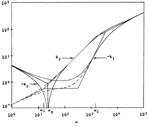
Fig. 3. Kmn-w diagram for a shock-excited gas experiment. =t = 4.5 103 U/m (Te=3. 5 eV); p = 1. 7 X 10- 5 kg/m3 (n=1.5X10 15/cc H+); B = 1. 6 w/m2; a = 0. 07 m; first axisymmetric mode; insulating wall.

o

gradient improperly in the momentum equation (3). When the pressure is properly taken into account, it is seen that the perturbation pressure is indeed zero for the TM modes (Eq. 25) but nonzero and non-negligible for the TE modes (Eq. 33), unless the density is very small. For liquid metals, this is clearly not the case.

Figure 3 is a graph similar to Fig. 2, but for parameters suitable to a gaseous dis-charge experiment. It also shows the effect of differing transverse and longitudinal conductivities.

b. EFFECTS OF NONIDEAL CONDITIONS

Three important factors not considered in prior investigations are the effects of viscosity, finite conductivity walls and transverse fields.

Viscosity was considered by Bluel6 in attempting to account for inconsistencies in the Lundquist4 and Lehnert3 experiments in which the walls were made of insulating

material. Because the ratio of electrical to viscous diffusivity is extremely large and the electromagnetic boundary conditions demand zero velocity at the walls, no significant

15

I__

_ __

__

effect of viscosity was found. However, if the walls are perfectly conducting, the elec-tromagnetic boundary conditions demand a maximum of velocity at the walls and some effect might then be expected. In Appendix A it is shown that again viscosity has no sig-nificant effect, the only alteration required being the addition of a thin (about 0. 01 cm thick at the frequencies of interest) transition region at the wall.

In Appendix A the effect of a transverse component in the DC field is treated. There it is shown that the only effect is to introduce a highpass cutoff. If this cutoff occurs at a frequency less than 2 (i. e., the transverse field is less than the longitudinal field), it is given by

2w262 2 2

Wco-(51)

where 6 is the ratio of transverse to longitudinal magnetic field. In Fig. 4 is shown an exact evaluation of the propagation constant for an NaK experiment, where 6 = 0. 1 with the curves for = 0 dashed in for comparison.

In Appendix A it is shown that a wall material of the same or lower conductivity as

103 102 101 100 10' 5 1

Fig. 4. Propagation constant with transverse field effect in NaK.

Boz = 8 kgauss; a = 6 in.; _{oz~~~~~~~~~~~~~~} 6 = 0. 1; ₂ = °.

16

I

I

_I_

that of the fluid acts very much as if it were a perfect insulator. But if the wall con-ductivity is much greater than that of the fluid, it approximates a perfect conductor.

0

-1

-2

-3

1 x/2 2 (T1a) 3 4 5

Fig. 5. Graphical solution of Eq. 52 for NaK. (a) Stainless-steel wall, a = 7.5 in.,

b = 0. 25 in.;

(b) Copper wall, a = 6 in., b = 0. 25 in.

This is illustrated in Fig. 5 in which a plane parallel waveguide is considered. Figure 5 is the graphical solution of

az b

tan (y1a)= a'a 1a),

I (52)

in which is the mode factor, a the half-width of the waveguide, b the wall thickness, a' the fluid conductivity, and 2 the wall conductivity. If the wall is a perfect insulator (-2=0), Y a = Tr; if it is a perfect conductor, y₁a = r/2. Two cases are shown, one for a stainless-steel wall (under the assumption of good electrical contact), and the other a

copper wall.

2.2 LOSSY HYDROMAGNETIC RESONATOR

In general, when a hydromagnetic resonator is excited electrically, the current from the injector will spread through the fluid and excite both a bulk motion and an Alfv6n wave. The division of energy between these two modes will depend on how close to a radial current sheet the exciting current is. This will, in turn, depend on both the

17

geometry of the electrode and the excitation frequency.

a. Small-Signal Waves

If, in Fig. 1, a length, , of the waveguide were cut out and terminated with insulating plates, it would act as a lossy half-wave resonator. It may be excited by a thin conducting ring set into one end as in Fig. 6. This situation may be approximated

Fig. 6. Hydromagnetic resonator with electrical exciter.

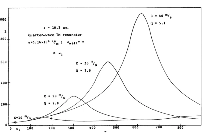
Fig. 7. Magnitude of Z as a function of frequency and Alfvdn speed.

18

" I

by a thin disk, insulated except for the edges. The exciting current will then be assumed to form a current sheet at the exciter end of the resonator, thereby exciting no bulk motion. Under these conditions, the electrical impedance seen at the terminals has been been found by Rink,2 4 and is for the lowest order mode

t

ik

z

It _{Z =-y-= z} Ta2r J 21 (a) _{cot kJ. (53)}

A plot of the magnitude of this impedance as a function of frequency is shown in Fig. 7 for the conditions of an experiment in NaK. Notice that only one resonance

0 2 4 6 8 10

o (kG)

Fig. 8. Resonance frequency as a function of magnetic field.

19

I

_ _

_ _

_

_I

_

occurs, and has a Q of, at most, approximately 5 for the conditions of a typical

experi-ment. The resonance frequency and its Q are plotted as functions of

mag-netic field in Fig. 8 for the same conditions. The resonance frequency for = c0 (Q = 0o) is also plotted. Notice that even though Q is quite low, the resonant frequency is quite close to the lossless case until one of the critical frequencies fl or f2 is approached. If

the resonance frequency is near f2, it will be higher than the lossless case and lower

if near fl. This effect is clearly due to the variation of Re [Kmn] from /c near the critical frequencies.

Near the resonance, an equivalent parallel RLC circuit may be found to approximate the terminal behavior. The parameters of this circuit (Appendix L) are

Trfa T J(Ta) e 21 C J (Tg) 2£ Jo2(Tg) L 2 (55) rr b T J (Ta) C2J2(Tg) R= 0 (56) e 2ra 2T4j2 (Ta) o rCFL a Q _2T2T ' (57)

where 1 < o << 2' For the region w 1 < << 2' the expression for Q may be obtained

only by solving a quadratic equation for w r; this results in a quite complex expression. The actual Q for all regions is presented in Figs. 7 and 8 from numerical evaluations of Z. For a typical set of data in an NaK experiment, C is 2200 farads, Le is ~5 X 10- 9

e henry, and Re is ~2 x 10 .

b. Bulk Effects

If the bulk of the exciting current spreads out through the fluid and if the fluid reacts as if it were a rigid body (with frictionless contact at the walls), the equation of motion would be

pa Z a

d 0 _0 grJr(r z) B r drdOdz, (58)

dt 0 0

where g is the radius of the exciter. The terminal voltage is given by

t = Bor d dr. (59)

20

Utilizing Eq. 58 and axisymmetry yield 2B (a2-g2 ) t a f

Vt 4 -o

§

pa4 0

Thus, at the terminals, this appears to be a capacitor: pa4

HM 2 a (61)

2B (ag ) Sg rJ rdrdz

0 r

If Jr is assumed to be of the form

-(z/L)

it e 6

~~~2aJ

r fL r/a

(1-et/ L ) 2waL

and if -L, the result is 2wa4

= 2aC f (63)

HM 2 22'

H o t ot(a -g 2

It is demonstrated in Appendix K that if B is considered nonuniform, then this should be modified by replacing C by the average C on the cross section.

o o

We have found that the equivalent circuit of a hydromagnetic resonator near res-onance consists of a large capacitor and a small inductance. The inductance is of the order of the quasi-static inductance with zero magnetic field. The resonant capacitance, however, is approximately 30 times greater than the bulk hydromagnetic capacitance

found in Appendix K. 4

CHM = 2 * (64)

~o Ave

Notice that the functional dependence on dimensions and magnetic field is exactly the same for Eqs. 54 and 64. The bulk hydromagnetic capacitance of Eq. 64 assumes solid body rotation of the fluid and therefore represents an upper bound on the actual capac-itance as seen from the terminals.

c. Step Response

Two cases may be distinguished in the response of a resonator to a step of current. The first case would occur if the losses are very low, that is, if conductivity is very high and viscosity is negligible. The exciting current would then tend to form a thin sheet near the exciter terminal and the principal effect would be an Alfven wave. The voltage at the terminal would look very much as in Fig. 9.

On the other hand, if the medium were quite lossy, the terminal current would spread out over the column of the resonator and excite the whole mass of fluid

21

simultaneously. The principal effect would then be a hydromagnetic capacitance. Since some Alfven wave would also be excited, the total response to a step of magnitude I at

Fig. 9. Step response of a low-loss Fig. 10. Step response of a lossy

hydro-hydromagnetic resonator. magnetic resonator.

the terminal should consist of a pedestal, because of the DC resistance, RDC, of the fluid, a ramp attributable to the hydromagnetic capacitance, CHM, and a damped

sinus-oid arising from the multiply reflected wave, as illustrated in Fig. 10. 2.3 NONUNIFORM MEDIA

Several types of nonuniform media problems may be considered. The conductivity, density, and magnetic field may be nonuniform, either singly or in combination. For example, several cases of nonuniformity may be considered for steady-state plasma experiments: (a) In a highly ionized gas of moderate density, the density dis-tribution is governed by diffusion and therefore varies from a peak value near the center of a tube to a low value near the walls. The electron temperature and, therefore, the electrical conductivity is nearly constant except near the walls. (b) In a weakly ionized gas of moderate density, the ionized particle density is controlled by diffusion modi-fied by the presence of neutrals. Neutral loading of the field lines by collision, how-ever, tends to make the density appear nearly uniform. The electrical conductivity, on the other hand, is directly proportional to the electron density and, therefore, varies over the cross section. (c) In a partially ionized gas, both the effective density and conductivity may vary over the cross section.

All of these possibilities are important, to some extent, in various experiments. Here only two types of nonuniformity will be considered: (a) radial variation of density, and (b) radial variation of an axisymmetric longitudinal magnetic field. In both cases it is practical to limit discussion to only the axisymmetric, transverse, magnetic field modes. These are also the modes of greatest experimental interest.

a. Radial Variation of Density p(r)

Under the assumptions noted above, the equations for b and ez can be

22

found (Appendix B). a [1 a rb] + 1 {co2-k2[c(r)+i]} bo 0 (65) 1 a ez = r (rb), (66) where 1 -= Magnetic diffusivity (67) o0 -B2 c (r) = p) Alfv6n speed (68) ~oP(r)

with the boundary conditions

be(a) = 0 Insulating wall (69)

ez4a) = 0 Conducting wall (70)

Notice that Eq. 65 is the same as Eq. 10 with n = 0 and p = p(r). Unless p(r) is specified very simply, however, there is no known solution for (65).

b. Radial Variation of Longitudinal Magnetic Field Bz(r)

Since the various space derivatives of the magnetic field are related through the curl and divergence relations, a transverse component, Br, must exist and both

com-ponents must be functions of r and z.

Bo(r, z) =irBor(r,z) + i B (r,z) (71)

With and p constant, the equation for b may again be found for axisymmetric TM modes (Appendix C).

(C+ic) ar- a (rb)] ac + C r a (rbe)

18

a

8

be

(eC

ac\

be

r

)+

~a

)

4-VoP

I

1 1__1_1__11__11_·_(_1_-

--

1_·---

---

·

---·--_-··1_1-.---1___1__

·

· ·

B (r, z)

Cz(r, z) = (74)

oP

Equation 72 appears to be extremely complex. Indeed it is not even separable. If, however, the magnetic field is assumed to be of a simple form with relatively weak variation, (72) may be considerably simplified (Appendix C).

The nonuniform magnetic field of the experiment was designed to be of the form (Appendix H)

Bo (r, z) = B 1 + (r/b) cos r (75)

B h (r/b) Z

B _or (r,z) = _Z7rb hb sin 2r _h (76)

b1 + (r/b)2

which satisfies the curl relation exactly and the divergence relation approximately. With b and h suitably large compared with the range of r and z, and by making the assump-tion that the waveguide will respond in the main to some average property of the longi-tudinal magnetic field, we have

iW.' 8 r (rb)1 + 2 Z [C2(r)+i ll}b 0, (77)

where effects due to the variation of CZ with z are also negligible (Appendix C). Notice

that Eq. 77 is now identical to Eq. 65.

c. Perturbation Expansion

The solution of Eqs. 65 and 77 is quite difficult for even the simplest c (r), since the result is complex hypergeometric functionals in which the unknown propagation con-stant, k, appears multiply. For more general c2(r), a closed-form solution is not possible. If, however, c (r) may be expressed as a power series in r, then a per-turbation expansion similar to those used in atomic physics2 9 may be used. That is,

00

c2(r) = c f rn(br)* (78)

n=O

Thus, the c2(r) approximating the situation of (75) is given by fo = f2 = 1, fl = 0 and

f = 0 for n > 2. n

Since all boundary conditions will be evaluated at the radius, a, it is convenient to define an expansion parameter as

d a (79)

b(so

that d = corresponds to a uniform field) and a normalized coordinate

(so that d = 0 corresponds to a uniform field) and a normalized coordinate

r

x

a (80)

Then if the variables of interest are expanded,

00o c2(x) = c2 _{fndnxn (81)} n=O 00 b(x) = bn(x) dn (82) n=O 00 ez(x) = en(x) dn (83) n=0 00 k2 = k2 P dn (84) o n n=0

Equating equal powers of d in (65) yields k iC 2 k 2 L(bn) =ko a k=l 2 k-m o f P rP x + ir- (85)

The equations represented by (85) are uncoupled from below, and thus may be solved sequentially. L is a linear differential (Bessel) operator defined as

dr= d 1 a2 2 62

L(b) [x (xbn)] + -kfoc+il)] b (86)

Since c (r) is symmetrical, fn = 0 for n odd. It may then be shown that bn , en , and Pn are also zero for n odd. Thus, for c (r), by approximating Eq. 75, Eq. 85 becomes

k2c2a2 L(b2n) b2(n-k) 2(k-1)x2+P2k +c2 ) (87)

o o k=O

The expressions for k2 derived from this expansion have been worked out to fourth order. For insulated walls,

r

1d

k2 = k

_o

1+ ic

2W Z

and for conducting walls,

25

[I. 1( + )( +_ ' (88)

r 2 k2 = k t1

-°l

2 2 oxZ 1 + i k y) 2 i (90) fZ + Z10 Z W02 where f 1

C

5

That is, f is a weighting factor on the field at r = 0 which represents taking a "linear" mean-square average of the field based on one-half the waveguide radius, rather than the volume mean-square average of the field given by

Zv 1 2f

f a

5 5 5

0

An exact numerical evaluation of the expression (Eq. 88) for insulated walls agrees very closely with the linear type average (within 1%) over the entire frequency range of interest for an NaK experiment. Equation 89 diverges, however. This difficulty was traced to a singularity in the differential equation for e. The position of this singularity

in frequency, radius, and expansion parameter may be predicted with accuracy by use

of the "linear" average rms Alfven speed to compute k. This was verified by an exact numerical evaluation of (89). Thus it may be concluded that for moderately nonuniform density or field, a liquid-metal Alfven waveguide with either conducting or insulating walls behaves very much as if it were a uniform waveguide having linear average prop-erties. In the final analysis, however, the correctness of linear averaging vs space averaging can only be settled by an experiment that must be precise, since the difference between the two kinds of averaging process should not amount to more than 4-6%.

III. EXPERIMENT

3.1 DESCRIPTION OF THE APPARATUS

Since the first prediction of magnetohydrodynamic waves by Alfv6n, in 1942, there has not been an experiment that demonstrated in a precise and unequivocal manner the properties of these waves. There has been no shortage of theoretical papers, but the formidable difficulties facing any experimenter in this area have kept the number of experiments small. These difficulties, such as those inherent in plasmas and the mar-ginal electrical properties and reactivity of liquid metals, have limited these experi-ments to demonstrations rather than precise verifications of the properties of Alfven waves. The experiment described here was undertaken as an attempt to rectify this situation. This experiment also provided a tool for verifying the results of the nonuni-form field theory presented in Section II.

3. 1. 1 Resonator

The objective of the resonator design was to provide a cylindrical waveguide of large diameter and long wavelength. These objectives were, of course, subject to limitations imposed by the magnet that would be used and the pole tips that would be used in forming the nonuniform field. Basically the resonator structure is a cylinder, 12 inches in diameter and 4 inches deep, with provisions for filling with NaK (78%/o potassium, 22% sodium) and for injecting currents in order to excite the various waves of interest.

The shell of the resonator, Figs. 11 and 12 (shown with the nonuniform-field pole tips), was constructed of 1/4" thick, nonmagnetic stainless steel, Heliarc welded through-out to eliminate the possibility of NaK leaking through-out or air leaking in. It was built in two almost identical mating parts in order to be compatible with the nonuniform pole tips (Figs. 11 and 12). The two halves of the resonator are sealed with a neoprene O-ring on the rim. The interior cylindrical wall is lined with a sheet of oxygen-free copper, 1/8" thick, to approximate a perfectly conducting boundary condition for the wave. The end walls are coated with a layer of cured "Eco-Bond" epoxy, 1/16" thick, to provide an insulated (open-circuit) termination at either end of the resonator. Filling and draining of the NaK is accomplished through two dry seat stainless-steel valves mounted at opposite sides of the shell on the rim. Pipes from the valves are welded into the wall at one end and directly opposite one another.

Electrical contact with the conducting fluid is made through ceramic and stainless-steel stand-off connectors (ADVAC 450-ES) welded into the shell at each end. An oxygen-free copper rod Welded to the end of each connector extends through the steel wall and epoxy layer. It is threaded to accommodate various types of exciters. In this experiment, a disk, 1/16" thick and 2" in diameter, insulated except for the edge, was used on each end. Two copper bars, insulated from the shell, terminating near the rim, conduct the excitation current to the center post of the connector and to the shell around the connector to ensure a symmetric current distribution. Current injected by the disk

a; o "o_a) o

r-10

r.

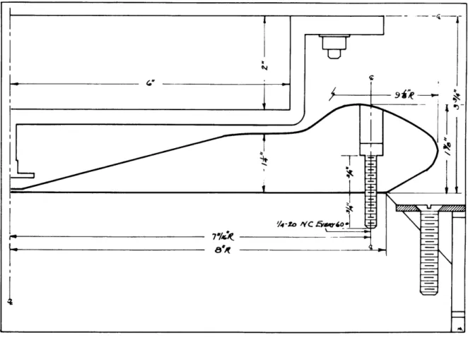
Fig. 12. Cross section of the magnet pole, nonuniform field pole, tips, and the resonator.

is collected on the copper wall and returned through the steel shell. 3.1. 2 Electronic Systems

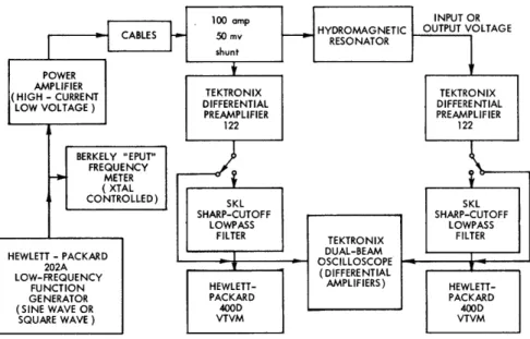
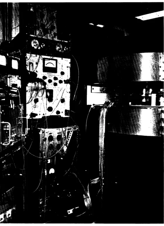
The arrangement of the main components of the electronics systems are dia-grammed in Fig. 13. The physical layout is shown in Fig. 14. The primary excitation of the entire system is provided by an HP 202A low-frequency function generator whose frequency is monitored by a Berkely "EPUT" meter counting on a crystal-controlled 10-second interval. _{Thus for the range of interesting frequencies, measurements may} be made to ±0. 1 cps or less than ±0. 1%. When the apparatus had been warmed up for 30 minutes, the combined drift of the oscillator and counter could not be detected in a 1-hour interval. The counter itself was calibrated against an oven-stabilized HP 524B counter and was found to have no detectable long-time drift.

The output of the oscillator is the input of a high-current, low-voltage amplifier specially designed and built for this application. This amplifier will provide a current of approximately 200 amps peak-to-peak to a load of 200 m, or less, over a frequency range of 1-2000 cps. The amplifier output section consists of 18 power transistors, in two banks of 9 each, operating in class B push-pull. Power supplies for the amplifier

Fig. 13. Electronic systems block diagram.

were a set of four 2-volt marine storage batteries and two electronically regulated low-voltage power supplies for the input stages. The storage batteries were sufficiently robust to allow full-power operation of the amplifier continuously for several hours. The output of the amplifier is fed to the resonator through two cables made of paralleled lengths of copper braid. The combined output resistance of the amplifier and the resist-ance of the cables and contacts amounted to some 5 mQ. The DC resistresist-ance of the reso-nator input -0. 1 m 2. Thus for direct-current operation the amplifier and cables appear to the waveguide tobe a current source. The wave impedance computed from Eq. 53 is in the vicinity of 1-10 iQ. Therefore, for Alfven waves, the driving system appears to be a quite good current source (within 0. 2o, at worst).

The driving current is measured with a standard 100-amp, 50-mv instrument shunt inserted in one of the cables. The shunt voltage and the input or output voltage of the res-onator are both monitored with Tektronix Type 122 differential preamplifiers. Differen-tial inputs are used to minimize the effects of ground loops, stray currents, 60-cycle pickup, commutator hash from the magnet generator, lead vibration and potential dif-ferences on the resonator case. To reduce the effects of lead vibration in the intense magnetic fields required for the existence of Alfven waves, the high-current leads were bound together as tightly as possible and wrapped with vibration damping material. The voltage pickup contacts were made directly on the connectors at the center of the res-onator and rigidly taped down while inside the field.

The single-ended output of the differential preamplifiers is then fed through Spencer-Kennedy Laboratories 200-cps sharp cutoff lowpass filters, displayed on a dual-beam Tektronix oscilloscope and measured with Hewlett-Packard 400D vacuum tube volt-meters. When step excitation is being used, the SKL filters are by-passed. With all units operating, the residual effective noise level was approximately 50 piv of 120 cps,

Fig. 14. Physical arrangement of the apparatus.

31

,, 17 ff -, -·s . !" 0~~9

which was apparently due entirely to the preamplifier power supplies. Thermal noise was negligible. The SKL filters are used to reduce the effect of third-harmonic cross-over distortion in the power amplifier.

3. 1. 3 Magnetic Field

The magnetic field was supplied by a Pacific Electric Motor Company iron core mag-net. The working volume of the magnet is a cylinder, 16" in diameter and 7 1/2" deep. The principal field is aligned parallel to the axis and is vertical. The cross section of a pole face is shown in Fig. 11. The magnet was designed to provide a maximum field of approximately 8500 gauss without pole tips for short periods with water cooling. Safety considerations dictated that kerosene be used as a coolant with some degradation of per-formance. A field current of 400 amps was required and was supplied by a rebuilt motor-generator set which was available. This field strength is enough to be in the region of Alfv6n waves. It was found, however, that by precooling the coils and pushing the gen-erator to a maximum output of approximately 525 amps, a field of up to 10, 700 gauss could be obtained for a few minutes. Heating was so strong at these power levels that the coil resistance increased rapidly, thereby reducing the current. A plot of magnetic

0 5 10 15 20 25 30

millivolts

Fig. 15. Saturation curves for uniform and nonuniform fields.

field as a function of current is presented in Fig. 15 (also millivolts across an 800-amp, 50-mv shunt). Over the central region of the field (0<r<6", -2"<z<+2")it varies less than 5% in radius and less than 0. 9% in height. The effect of the iron yoke was examined

and found to be negligible.

The nonuniform field was obtained by the use of shaped pole tips made of 100% pure iron (Armco) to minimize saturation effects. The contour of the pole tips was selected to yield a longitudinal (Bz) field that varied as in Eq. 75, with the smallest possible variation in the z direction and a minimal radial (Br) field, while keeping the largest possible variation of B in the radial direction. Typical results are illustrated in Fig. 16 with the fitted prediction of Eqs. 75 and 76 for comparison. A plot of B at r = 0" and at r = 2" as a function of magnet current is shown in Fig. 15. The hysteresis effect is also shown.

-1 0 1 2 5 6 7 8

Fig. 16. Radial variation of B and Br._{z r}

When uniform fields were being used, the resonator was mounted on an alu-minum stand so that its center was exactly at the center of the field volume. That is, z = 0, r = 0 was 3 3/4" from the pole faces. When a nonuniform field was being used, the resonator was held by brass screw jacks bearing on the pole tip mounting screws. Magnet current was measured by a Leeds and Northrup

33

potentiometer and an 800-amp, 50-mv shunt. 3.2 EXPERIMENTAL PROCEDURES

3. 2. 1 Resonance Measurements

Before starting a resonance frequency measurement, the magnet was precooled from 1 1/2 to 2 hours to make certain that the copper coils had reached minimum tempera-ture. All electronic systems were turned on, allowed to warm up, and thoroughly checked for malfunctions and drift.

To start a run, the resonator drive current was set to 22 amps rms and monitored to be sure it remained constant during the run. The magnet was turned on a allowed to

stabi-lize at the highest possible current. The current was then reduced to 31.05 my as indicated on the potentiometer, and allowed to drift downward to 30.95 mv as the coils heated. This meant that approximately 15 seconds were available in which to find the peak of the reso-nance curve in the output voltage by scanning the HP function generator frequency. The

current was then reduced to 29.05 mv, and the measurement repeated. This procedure was repeated until a resonance could no longer be detected. Smaller steps were not taken, because of a total time limitation imposed by the temperature rise of the magnet. In order to eliminate the effects of hysteresis, the current was always reduced in a con-tinuous fashion so that only the upper branch of the hysteresis curve was used.

These runs were repeated in a period of 3 days with several hours between runs. This was done to allow for adequate precooling of the magnet, to make sure that chance circumstances were not affecting the data and to get a measure of how much all of the indeterminate factors contributed to scattering of the data.

3. 2. 2 Step Response

Step response was obtained by using the square-wave output of the function generator at low frequency (10 cps). Polaroid Land camera photographs were taken of the input and output voltage waveforms for decreasing magnetic fields.

In order to examine the Alfven wave part of the waveform more closely, the output signal was fed to one side of the oscilloscope differential amplifier and a highpass fil-tered version of the current waveform was fed to the other. By adjusting the time con-stant of the filter (incorporated into the Tektronix preamplifier) and its amplitude, the ramp could be subtracted out. The remaining damped sinusoid was then expanded and amplified for close observation and recording.

3. 2. 3 Field Measurements

All field measurements were made with a Rawson-Lush rotating-coil gaussmeter. The curves presented in Fig. 15 were obtained by carefully centering and aligning the gaussmeter probe and rigidly fixing it in the magnetic field. The field was then varied as in the resonance measurements. Complete profiles of the magnetic field were made

34

by sliding the gaussmeter along a calibrated wooden track aligned on a radius, wedged and levelled at various heights. The precision of the magnet current setting was relaxed to ±0. 1 my, because of the necessity for a longer measurement interval and the low sensitivity of the gaussmeter indicator, as compared with the digital-frequency

meas-urement. Small resetting of the current was allowed, but hysteresis did not show up in the data.

3.3 SUMMARY OF RESULTS The results of the

frequencies, total step

experiments fall into several distinct groups: resonance

response, Alfven wave part of the step response, and

0 2 4 6 8 10

B o (kG)

Fig. 17. Half-wave resonance frequencies as measured.