Failure risk management of buried infrastructure using fuzzy-based techniques

Publisher’s version / Version de l'éditeur:

Journal of Water Supply Research and Technology: Aqua, 55, March 2, pp. 81-94, 2006-03-01

READ THESE TERMS AND CONDITIONS CAREFULLY BEFORE USING THIS WEBSITE.

https://nrc-publications.canada.ca/eng/copyright

Vous avez des questions? Nous pouvons vous aider. Pour communiquer directement avec un auteur, consultez la première page de la revue dans laquelle son article a été publié afin de trouver ses coordonnées. Si vous n’arrivez pas à les repérer, communiquez avec nous à PublicationsArchive-ArchivesPublications@nrc-cnrc.gc.ca.

Questions? Contact the NRC Publications Archive team at

PublicationsArchive-ArchivesPublications@nrc-cnrc.gc.ca. If you wish to email the authors directly, please see the first page of the publication for their contact information.

NRC Publications Archive

Archives des publications du CNRC

This publication could be one of several versions: author’s original, accepted manuscript or the publisher’s version. / La version de cette publication peut être l’une des suivantes : la version prépublication de l’auteur, la version acceptée du manuscrit ou la version de l’éditeur.

Access and use of this website and the material on it are subject to the Terms and Conditions set forth at

Failure risk management of buried infrastructure using fuzzy-based techniques

Kleiner, Y.; Rajani, B. B.; Sadiq, R.

https://publications-cnrc.canada.ca/fra/droits

L’accès à ce site Web et l’utilisation de son contenu sont assujettis aux conditions présentées dans le site LISEZ CES CONDITIONS ATTENTIVEMENT AVANT D’UTILISER CE SITE WEB.

NRC Publications Record / Notice d'Archives des publications de CNRC:

https://nrc-publications.canada.ca/eng/view/object/?id=0f628e58-1c73-409d-a58c-7408c9ff2b8e https://publications-cnrc.canada.ca/fra/voir/objet/?id=0f628e58-1c73-409d-a58c-7408c9ff2b8e

http://irc.nrc-cnrc.gc.ca

Fa ilure risk m a na ge m e nt of burie d

infra st ruc t ure using fuzzy-ba se d

t e chnique s

N R C C - 4 8 3 1 9

K l e i n e r , Y . ; R a j a n i , B . ; S a d i q , R .

A version of this document is published in / Une version de ce document se trouve dans:

Journal of Water Supply Research and Technology : Aqua, v. 55, no. 2, March 2006, pp. 81-94

Failure risk management of buried infrastructure using

fuzzy-based techniques

1

Yehuda Kleiner, 2Balvant Rajani and 3Rehan Sadiq

1*

Senior Research Officer and Group Leader

Institute for Research in Construction, National Research Council Canada (NRC), 1200 Montreal Road, Building M-20

Ottawa, ON, Canada K1A 0R6

Yehuda.Kleiner@nrc-cnrc.gc.ca

Phone: 1-613-993-3805 Fax: 1-613-954-5984

2

Principal Research Officer

Institute for Research in Construction, National Research Council Canada (NRC), 1200 Montreal Road, Building M-20

Ottawa, ON, Canada K1A 0R6

Balvant.Rajani@nrc-cnrc.gc.ca

Phone: 1-613-993-3810 Fax: 1-613-954-5984

3

Research Officer

Institute for Research in Construction, National Research Council Canada (NRC), 1200 Montreal Road, Building M-20

Ottawa, ON, Canada K1A 0R6

Rehan.Sadiq@nrc-cnrc.gc.ca

Phone: 1-613-993-6282 Fax: 1-613-954-5984

Failure risk management of buried infrastructure using

fuzzy-based techniques

ABSTRACT: The effective management of failure risk of buried infrastructure assets requires knowledge of their current condition, their rate of deterioration, the expected consequences of their failure and the owner’s (decision-maker) risk tolerance. Fuzzy-based techniques seem to be particularly suited to modeling the deterioration of buried infrastructure assets, for which data are scarce, cause-effect knowledge is imprecise and observations and criteria are often

expressed in vague (linguistic) terms (e.g., ‘good’, ‘fair’ ‘poor’ condition, etc.). The use of fuzzy sets and fuzzy-based techniques helps to incorporate inherent imprecision, uncertainties and subjectivity of available data, as well as to propagate these attributes throughout the model, yielding more realistic results.

This paper is the second of two companion papers that describe an entire method of managing risk of large buried infrastructure assets. The first companion paper describes the deterioration modeling of buried infrastructure assets, using a fuzzy rule-based, non-homogeneous Markov process. This paper describes how the fuzzy condition rating of the asset is translated into a possibility of failure. This possibility of failure is combined with the fuzzy failure consequences to obtain fuzzy risk of failure throughout the life of the pipe. This life-risk curve can be used to make effective decisions on pipe renewal. These decisions include when to schedule the next inspection and condition assessment or alternatively, when to renew a deteriorated pipe, and what renewal alternative should be selected.

1 Introduction

To run an effective risk management program one needs to be able to predict failure risk levels throughout the life of the asset. Lawrence (1976) defined risk as a “measure of probability and severity of negative adverse effects”. In a companion paper, Kleiner et al. (2006), introduced a method to model the deterioration of large buried infrastructure assets as a rule-based, non-homogeneous fuzzy Markov deterioration process. This deterioration model yields a family of curves depicting the condition rating of the asset (in terms of membership values to defined condition states) at selected point along the life of the asset. This paper describes the following five steps in assessing and managing the risk of asset failure:

a) How to convert the fuzzy life deterioration curve into possibility of failure.

b) How to combine the possibility of failure with failure consequences (expressed as a fuzzy set) to obtain a life-risk curve.

c) How to make a decision on whether to renew, rehabilitate or replace an asset or schedule its next inspection, based on the decision maker’s risk tolerance.

d) How to use expert opinion to assess the renewal condition rating as well as the post-renewal deterioration rate of the asset.

e) How to select a renewal alternative based on this post-renewal performance assessment. The proposed fuzzy-based risk modeling and decision process is especially suited for assets for which data are scarce, and when available are often imprecise and vague. These assets are

typically difficult to access and expensive to inspect. In this paper, data on buried, large-diameter water transmission mains are used to demonstrate all the aspects of the proposed method.

2 Fuzzy risk of failure

2.1 Possibility of failure

Kleiner et al. (2006) proposed a fuzzy rule-based Markov process to model infrastructure asset deterioration. They used a seven-grade (condition states) fuzzy set (excellent, good, adequate,

formulated such that the condition of the asset at any given time could have significant

memberships to no more than three contiguous condition states. It should be noted that the failed (state 7) condition state does not mean that collapse or rupture has already happened (in which case the membership would be a definite unity), rather that the asset is in such a bad condition that failure is imminent and can occur at any time as a result of the slightest perturbation.

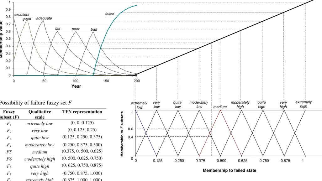
Further, since fuzzy subsets (such as triangular fuzzy numbers - TFNs) are often interpreted (Klir and Yuan, 1995) as possibility distributions (in contrast to probability distribution), it follows that the membership to the failed state at any given time can be viewed as the possibility (not probability) of failure at that time (see brief discussion about probability versus possibility in Kleiner et al., 2006). The family of curves depicting the condition rating of the asset at every point in its life is illustrated at the top left portion of Figure 1.

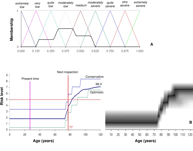
A nine-grade fuzzy set F (from extremely low to extremely high) defined for the possibility of failure is illustrated at the bottom right of Figure 1. The membership values to the failed state in each time step are fuzzified (or re-mapped) on to this fuzzy set F, as illustrated in Figure 1. This re-mapping of a membership value onto a secondary fuzzy set is similar to the concept of “type-2 fuzzy sets” (Mandel and John, 2002). For example in Figure 1, membership of 0.45 to the failed state translates to 0.4 membership to moderately low and 0.6 membership to medium possibility of failure, or in a vector form (0, 0, 0, 0.4, 0.6, 0, 0, 0, 0). The possibility of failure can be computed for each year t in the life of the asset. This possibility of failure along the life of the asset is used to generate a fuzzy life-risk curve as is described later.

2.2 Fuzzy consequences of failure

The failure consequences of buried infrastructure assets such as large-diameter pipes can be substantial. They may comprise direct costs (emergency repair, direct damage to adjacent assets, liability), indirect costs (loss of production, accelerated deterioration) and social costs (disruption of business, loss of confidence, loss of time). Some research on how to assess these costs has been reported in the literature (e.g., Cromwell et al., 2002; PPK Consultants, 1993) but it appears that much more work is required, and detailed case studies can help alleviate the lack of good data. A well-structured process of querying local experts and practitioners could be devised to interpret qualitative knowledge into fuzzy numbers. One possible approach is to develop a process based on fuzzy synthetic evaluation similar to that applied by Rajani et al. (2006) to

translate distress indicators to condition ratings. However this issue is beyond the scope of the research described here.

In this paper it is assumed that the severity of asset-failure consequences can be provided through the fuzzy set Q, which comprises nine severity grades (triangular fuzzy

numbers/subsets) that include extremely low, very low, quite low, moderately low, medium,

moderately severe, quite severe, very severe and extremely severe. The utility is thus assumed to be able to provide a fuzzy set representing failure consequences. For example, the fuzzy set (0, 0, 0.2, 0.8, 0, 0, 0, 0) represents an asset whose failure consequences has 20% membership to quite

low and 80% membership to moderately low. The severity ratings of failure consequence can be subjective, e.g., the loss of service to one thousand customers in a small municipality might be perceived as very severe, while the same loss of service in a large city would be described as

quite low. It should also be noted that the fuzzy set representing failure consequences must be convex and must have unit cardinality, i.e., sum of memberships in a fuzzy set is equal to 1.

2.3 Fuzzy risk of failure

As stated in the introduction, failure risk is a measure of the probability and severity of failure. Often failure risk cannot be treated with mathematical rigour during the initial or screening phase of decision-making (Lee, 1996), especially when a complex system involves various

contributory risk items with uncertain sources and magnitudes.

Let fuzzy set Z, representing failure risk, be defined by nine triangular fuzzy subsets. These subsets represent the nine failure risk levels extremely low, very low, quite low, moderately low,

medium, moderately high, quite high, very high and extremely high. The rule-set RZ that governs

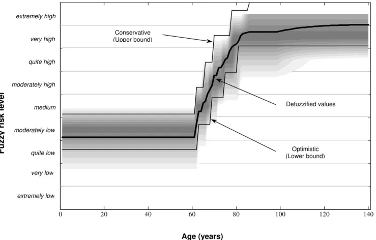
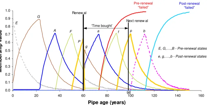
the relationship between failure possibility (set F), failure consequence (set Q) and failure risk (set Z) is given in Table 1. The Mamdani (1977) algorithm, detailed in the companion paper Kleiner et al. (2006) for the multiple input single output (MISO) model, is used to compute the fuzzy risk (output) from the inputs of fuzzy possibility and fuzzy consequences of failure. As the possibility of failure can be calculated for each year t in the life of the asset, it can be combined with the fuzzy consequences of failure to obtain a fuzzy risk curve for the life of the asset, as illustrated in Figure 2. The intensity of the grey levels in Figure 2 represents the

membership values to the respective risk levels. The black curve represents the defuzzified risk values, which are akin to the mean risk level. It can be seen that the defuzzified values do not always coincide with the highest membership (modal) values, which means that the fuzzy set that represents risk at any year t is not necessarily symmetrical about its mode.

Kleiner et al. (2006) described the concept of a possibilistic confidence band (constructed using α-cuts). The same concept is used to construct a confidence band for the life-risk curve, as illustrated in Figure 2 for α = 0.25. In this example, the band defines the ranges at which

membership values to any risk grade are greater or equal to 0.25. In other words, within this band are all those risk levels to which the modelled asset has membership of at least 0.25. Naturally, the confidence band will become narrower as the value of α increases. Conversely, for α = 0 the confidence band will encompass the entire possibility spectrum (support of the fuzzy set). It is clear that the upper bound of the band represents a more conservative attitude, while the lower bound represents a more optimistic attitude. It is worth reiterating here that the

possibilistic confidence band cannot be interpreted in the same way as a probabilistic confidence band, as it provides a notional rather than a frequentist-based quantitative idea about the

likelihood of the ‘best estimate’ prediction to be in the corresponding interval. Further, there generally is no ‘standard’ α value used for this type of analysis (analogous to, say, 90% or 95% confidence level in probabilistic analysis. This possibilistic confidence band is used in the decision process as discussed later.

3 Decision-making

process

Ideally the optimal strategy of renew/repair/inspect will be the one, which minimizes the present value of the total life-cycle costs (including direct, indirect and social costs of failure) that are associated with the asset. This strategy requires accurate forecasting of the asset deterioration and its probability of failure over its life cycle, as well as of the expected consequences of failure. Additionally, it requires the forecasting of asset deterioration and probability of failure after rehabilitation or renewal, which may change the characteristics of the renewed asset and its behaviour.

Several decision-making strategies for various infrastructure assets have been described in the literature. Examples that include WRc (1993, 1994), Edmonton (1996) and Zhao and McDonald (2000), provide guidance for inspection frequency of sewers. These guidelines are largely qualitative and prescriptive, e.g., “condition x requires that the asset be inspected every y years”, and as such tend to provide a rather broad and general range of actions with only an implicit consideration of deterioration rates. However, these guidelines have gained significant popularity because of their simplicity and their need for few data. Other, researchers have proposed more elaborate and quantitative methods, e.g., Madanat and Ben Akiva (1994), Li et al. (1995, 1997), Pandey (1998), Hong (1998), Jiang et al. (2000), Kleiner (2001), and Guillaumot et al. (2003). These, however, do not seem to have gained much popularity, possibly because underlying models are either too complex or are data hungry, or both.

Traditional quantitative approaches to decision-making present some limitations in the data-poor realm of buried infrastructure. The first limitation is the requirement for sufficient data to train the underlying deterioration models. The second is that, in order to evaluate a renewal

alternative, post-renewal deterioration (for which typically no data exist) has to be evaluated. The third is that, the subjectivity and vagueness in the determination of the asset condition, as well as the consequences of failure, are not considered.

In the proposed fuzzy rule-based approach described in this paper, calculations of life cycle costs are not crisp, and ‘true probabilistic’ values for failure occurrences are not determined explicitly. Consequently, the traditional concept of discounting of future costs (present value of stream of costs) cannot be explicitly applied and life-cycle costs of various renewal alternatives cannot be directly compared.

3.1 Criterion for renewal or scheduling next inspection/condition assessment

A maximum risk tolerance (acceptable risk) value is proposed as a decision criterion, since the life-cycle costs of various alternatives cannot be directly compared. A water utility, through a consensus-building process like Delphi (Linstone and Turoff, 2002) or other, will define its maximum risk tolerance (MRT) zmax for its infrastructure asset. In the present context, maximum

risk tolerance zmax will be one of nine risk-level of the fuzzy set Z. Since the term risk is a

zmax will suffice for the entire inventory of large-diameter transmission mains. At the same time,

special consideration(s), which might not be readily integrated into the set of factors that determine failure consequences, may render more than one zmax necessary.

It is assumed that any decision about renewal of the asset will always be preceded by an inspection and condition assessment. Thus, if the deterioration model of an asset predicts that

maximum risk tolerance zmax is going to be reached at year tz, it follows that at year tz (or

thereabouts) an inspection/condition assessment will be scheduled. This inspection/condition assessment can have one of two outcomes: either the observed condition of the asset is better than predicted, i.e., the deterioration model overestimated the deterioration rate, or the observed condition of the asset is the same or worse than the model predicted i.e., the deterioration model was accurate or underestimated the deterioration rate. In the case of the former outcome, the deterioration model needs to be calibrated to include the newly acquired data, and then re-applied to obtain a new tz. If it is the latter outcome, renewal work has to be planned immediately

and implemented as soon as possible.

The decision maker’s tolerance (attitude) for risk can be expressed in two independent manners. First, as was described earlier in this section, the decision maker provides an explicit measure of

maximum risk tolerance zmax. Second, the decision maker can select the α-level of the

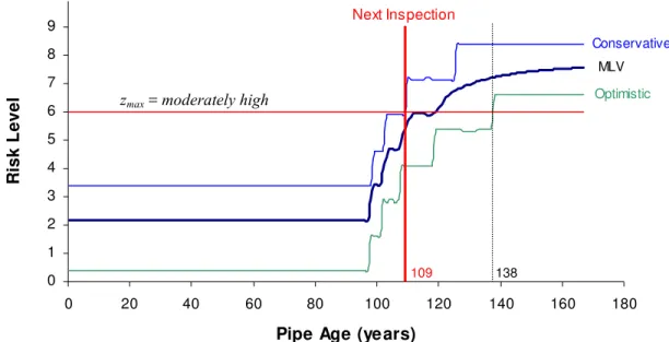
possibilistic confidence limit. As discussed earlier, the confidence band will become wider (and the higher the confidence) as the α-cut value decreases. Consequently, a decision maker with a conservative attitude increasingly makes more conservative decisions as the selected α-cut is lowered. Figure 3 illustrates an example in which the MRT (zmax = moderately high) is forecasted

to be met between 109 and 138 years of age at an α-value of 0.6. The conservative decision maker will schedule the next inspection/condition assessment to occur at the asset age of 109 years.

3.2 Examination and comparison of renewal alternatives

As described earlier, the comparison of renewal alternatives requires the knowledge (or assumptions) about the expected performance of the asset after renewal. It is assumed that this post-renewal expected performance can be determined by (a) the post-renewal condition of the asset (i.e., the degree of improvement), and (b) the post-renewal deterioration rate of the asset.

3.2.1 Evaluation of post-renewal condition

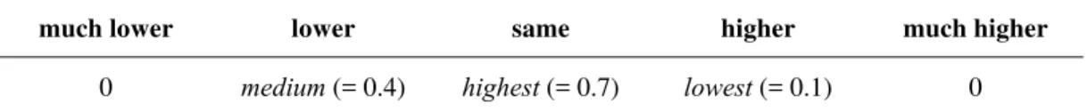
Renewal of an asset should invariably lead to the improvement of its condition rating. Typically, the shift in the condition rating from before to after renewal will depend on factors such as technology, material, process, etc. of the specific renewal alternative. Quantitative information on how a specific renewal alternative improves the condition rating is most often unavailable because the renewal alternatives are based on technologies that are relatively new and conditions under which they are applied can vary. A raw condition improvement matrix, P’k, is introduced

to formalize a process for making educated judgments about the shift of condition state from before to after the application of renewal alternative k.

In the absence of sufficient field data to assign deterministic or even probabilistic values, the raw condition improvement matrix, P’k, is constructed based on expert opinion, where linguistic

terms, e.g., highest, medium, and lowest are used to capture the belief of experts about a shift from one condition state to another, as is illustrated in Table 2. In turn, each of these linguistic terms can be assigned relative weights, say, 0.7, 0.4 and 0.1, respectively (every row in P’k must

be convex). Once the linguistic terms are substituted by the corresponding weights, the raw condition improvement matrix, P’k, is normalized so that the sum of weights in each row equals

unity, to obtain the normalized condition improvement matrix, Pk:

∑

were pi,j is a member of matrix Pk and p’i,j is a member of matrix P’k. In the example depicted in

Table 2 k P = ⎥ ⎥ ⎥ ⎥ ⎥ ⎥ ⎥ ⎥ ⎥ ⎦ ⎤ ⎢ ⎢ ⎢ ⎢ ⎢ ⎢ ⎢ ⎢ ⎢ ⎣ ⎡ ⇒ ⎥ ⎥ ⎥ ⎥ ⎥ ⎥ ⎥ ⎥ ⎥ ⎦ ⎤ ⎢ ⎢ ⎢ ⎢ ⎢ ⎢ ⎢ ⎢ ⎢ ⎣ ⎡ 0 0 0 0.333 0.583 0.083 0 0 0 0.083 0.588 0.333 0 0 0 0.333 0.583 0.083 0 0.267 0.467 0.267 0.083 0.583 0.333 0.125 0.875 000 . 1 0 0 0 0.4 0.7 0.1 0 0 0 0.1 0.7 0.4 0 0 0 0.4 0.7 0.1 0 0.4 0.7 0.4 0.1 0.7 0.4 0.1 0.7 0.7 (2)

where the left matrix is the raw condition improvement matrix, P’k. The post-renewal condition

rating of the asset is obtained from equation (3) as follows:

k t k k t C P C = • ₍₃₎

where the operator • indicates a simple matrix multiplication and tk

denotes the time of renewal alternative k. The post-renewal condition has a cardinality of unity, i.e., the sum of all its members, which are membership values, equals unity. The renewal process itself is assumed to be instantaneous (with respect to the length of a time step which is typically one year), where

denotes the asset condition immediately after renewal, and k tk C k tk Cr k tk

Cs the asset condition

immediately before renewal. For example, suppose that at age 60 the condition rating of an asset is Ct=60 = (0, 0, 0, 0.3, 0.5, 0.2, 0). If condition improvement matrix Pk from Table 2 is applied

the resulting post-renewal condition rating becomes k tk

Cr ₌₆₀ = (0.12, 0.50, 0.36, 0.02, 0, 0, 0).

Let the term post-renewal equivalent age, τk, be defined as the age of the asset, prior to renewal, at which its condition was equal (or very close to) to the post-renewal condition . Post-renewal equivalent age τ

k tk Cr r r r k

is found by minimizing the sum of square deviations between Ct=τ and

as depicted in k tk C (4):

∑

where is the membership value in condition state i (i = 1, …, 7) of the post-renewal condition rating (when renewal alternative k was implemented at time t

k i k C t r μ k tk C k) and is the

membership value in condition state i (i = 1, …, 7) of the pre-renewal fuzzy condition rating (τ i k C τ μ k C_τ κ

< tk). This means that renewal option k made the asset functionally ‘younger’ by (tk - τκ)

years.

In the example above, the post-renewal condition rating of the asset is

= (0.12, 0.50, 0.36, 0.02, 0, 0, 0). Suppose that searching through all the pre-renewal k

tk

C

60 =

condition ratings of the asset Ct(t =1, ..., 60) it is found that

= (0.093, 0.533, 0.374, 0, 0, 0, 0) has the closest match of membership values to , i.e., the minimum sum of square deviations between corresponding membership values. Consequently, τ 24 = t C k tk C 60 =

k _{= 24 years (the asset is as good as it was at age 24) and renewal alternative k}

made the asset functionally ‘younger’ by (tk-τκ) = 36 years.

3.2.2 Evaluation of post-renewal deterioration

Once an asset segment has been renewed, it will undergo deterioration at a rate that may be the same or different from the asset segment before it was renewed. How slow or fast the renewed asset segment will deteriorate will largely depend on the characteristics of the selected renewal alternative. For a fair comparison between candidate renewal alternatives, the post-renewal deterioration rate must also be considered. However, for lack of available field data this evaluation must also be based on expert opinion.

Similar to the condition improvement matrix, expert opinion is solicited to provide input on how the expected post-renewal deterioration rate will be relative to the deterioration rate observed prior to renewal. This expert opinion is expressed in the same linguistic terms used for the raw condition improvement matrix. Let B denote a 5-tuple fuzzy set (much lower, lower, same,

higher, much higher) as shown in Figure 4. The fuzzy number BBk is used to evaluate the

post-renewal deterioration rate of post-renewal alternative k relative to the observed (or historical)

deterioration rate (Table 3), similar to the manner in which P’k. is used to evaluate post-renewal

condition rating. For convenience, the confidence in each of the elements of the BkB is expressed

using the same linguistic terms (and relative weights) as those used for P’k. Once the expert

expresses belief on anticipated post-renewal deterioration rates, these linguistically expressed beliefs are substituted for their respective weights, which are mapped on fuzzy set B, as is shown Table 3. Subsequently, BBk is defuzzified (using the centre of area method) to obtain the

post-renewal relative deterioration factor bk. In the example illustrated in and , the

linguistic input in is substituted by the respective weights to obtain

Bk

Table 3 Figure 4 Table 3

B = (0, 0.4, 0.7, 0.1, 0), which is then mapped onto B (Figure 4) and defuzzified to obtain the

post-renewal relative deterioration factor bk (= 0.944). Note that the solid line in Figure 4 is a

The renewal deterioration is modelled as if the asset continues to deteriorate from the post-renewal equivalent age, τk, using the pre-renewal deterioration rate, k

t

D_=τ , modified by the

post-renewal relative deterioration factor bk, i.e., the asset continues to deteriorate through the same

deterioration process described in the companion paper Kleiner et al. (2006). The only difference is that all the defuzzified deterioration factors t are multiplied by the scalar b

j i

D_, k. In the above

example, applying bk = 0.944 will yield a post-renewal deterioration rate that is somewhat lower

than the pre-renewal rate.

3.2.3 Quantification of post-renewal performance

Let Tk be defined as the time interval it would take for the renewed asset (renewal alternative k)

to reach condition C_tkk, which is its pre-renewal condition. It can be said colloquially that T s

k is

the time interval which renewal alternative k ‘bought’ for the asset, or in other words, it is the time interval by which the subsequent renewal can be deferred. Similar to τk, Tk is found by

minimizing the sum of square deviations between k _T and

k k C_{τ +} k tk Cs as depicted in equation (5):

∑

where is the membership value in condition state i (i = 1, …, 7) of the pre-renewal condition rating (when renewal alternative k was implemented at time t

k i k C t s μ k tk Cs k); is the

membership value in condition state i (i = 1, …, 7) of the post-renewal fuzzy condition rating . In the example above T

i k k C T + τ μ k k T

C_{τ +} k= 40 years, which means that the asset in the example is

expected to return to its pre-renewal condition rating 40 years after renewal alternative k has been applied.

3.2.4 Selection of a renewal alternative

As was noted earlier, each renewal alternative k is associated with a condition improvement matrix Pk, and a post-renewal deterioration rate. Additionally, each renewal alternative will also

until the next expected renewal, the magnitude of Tk is determined by the extent to which the

asset condition is expected to improve under the expected post-renewal deterioration rate. Assuming that all renewal alternatives will restore the functionality equally well during their respective expected Tk periods, the only criterion for the selection of the best renewal alternative

can be cost versus time ‘bought”, or more precisely, the preferred renewal alternative will be that for which the ratio Sk/Tk is the lowest. If different renewal alternatives are anticipated to provide

different levels of functionality then additional functionality criteria need to be defined and quantified for all the renewal alternatives. However, this issue is beyond the scope of this research.

4 Example

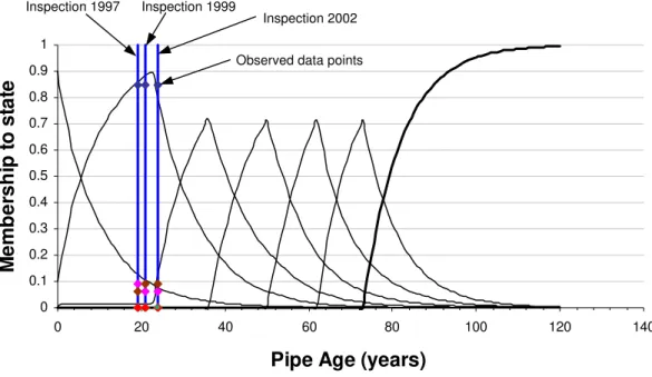
The data and results presented in the companion paper (Kleiner et al., 2006) are used here to illustrate the application of concepts developed in this paper. This example referred to one of several 96” (2400 mm) diameter PCCP pipe segments that belong to Arizona Public Service Company (APS). This PCCP pipe segment was installed in 1978 and inspected in 1997, 1999 and 2002. Kleiner et al. (2006). For the example presented here, the deterioration model was trained on all three condition ratings established from observed distress indicators and the

modelled condition rating of the pipe in 2002 (age 24) was obtained as = (0.08, 0.8, 0.13, 0, 0, 0, 0) with SSD (sum of squared deviations) = 0.017. The base deterioration rate parameter was found to be d

24 = t

C

0 = 0.054. The resulting deterioration curves together with the failed curve are

shown in Figure 5. Note that threshold values for condition states 3, and higher were assumed to be 0.7.

The following sub-sections are structured to correspond to each of the five steps involved in the assessment and management of failure risk that are enumerated in the introduction.

4.1 Convert fuzzy deterioration to possibility of failure

The failed curve obtained in the example discussed above was re-mapped onto the failure possibility fuzzy set (set F) using the process illustrated in Figure 1. This mapping was

conducted for each year in the life of the pipe. It can be seen in Figure 5 that membership to the

its possibility of failure to be (1, 0, 0, 0, 0, 0, 0, 0, 0), i.e., extremely low, and increases after 72 years until it reaches extreme values at ages beyond 100 years.

4.2 Combining possibility and consequences of failure to obtain risk

The fuzzy consequences of failure were arbitrarily assumed to be Q = (0, 0, 0.2, 0.5, 0.3, 0, 0, 0, 0), i.e., predominantly moderately low with lower memberships to medium and quite low. The graphical representation of the fuzzy consequences is illustrated in Figure 6A. The fuzzy consequences (set Q) and failure possibility (set F) were then combined, using the Mamdani (1977) algorithm with the rule base provided in Table 1, to obtain the fuzzy risk for every year in the life of the pipe, as shown in Figure 6B (on the right).

4.3 Decision: renew or schedule next inspection

It was arbitrarily assumed that decision maker has a maximum risk tolerance zmax medium, and a

moderately conservative attitude which requires a confidence band of 50% (α value of 0.5). Figure 6B (left) illustrate that zmax is anticipated to be exceeded at age of about 77 years, based

on this moderately conservative attitude (if an optimistic attitude were taken, zmax would be

anticipated to be exceeded about 15 years later). Consequently, the next inspection/condition assessment would be scheduled to that age and the resulting condition rating compared to condition rating that was predicted by the model for that age. If the newly observed condition rating indicates that the pipe is in a better condition than predicted, the model will need to be re-calibrated using the new data (the newly observed condition rating) and the subsequent

inspection will then be scheduled. If, on the other hand, the observed condition rating is worse or the same as that predicted by the mode, renewal works should be implemented as soon as

possible.

4.4 Assessment of post-renewal condition rating and deterioration factor

Suppose that the utility had contemplated the implementation of external post-stressing of the PCCP pipe at an age of, say, 60 years. (earlier than the anticipated age to reach zmax) due to an

unexpected change in attitude. This renewal action is referred to here as renewal alternative k =1. In accordance with the trained model (Figure 5) the condition rating of the pipe at that age is predicted to be approximately Cs₆₀1 = (0, 0, 0.1, 0.3, 0.6, 0, 0), i.e., predominantly poor. Suppose

further that the condition improvement matrix P1 for renewal alternative 1 can be extracted based

on expert opinion depicted in Table 2. The post-renewal condition rating of the pipe is found by applying equation (3), i.e., 1 ₁

60 1

60 C P

Cr = s ⊗ = (0.1, 0.4, 0.5, 0, 0, 0, 0). Applying equation (4) will

reveal that the expected equivalent age of the pipe post-renewal is τ1 = 30 years, i.e., post-renewal condition rating is such that the pipe has been rejuvenated to an age of 30 years.

Suppose further that the post-renewal deterioration rate for renewal alternative 1 can be extracted based on expert opinion depicted in Table 3. The post-renewal deterioration factor will therefore be the same as determined in Figure 4, i.e., bk=1 = b1 = 0.944.

4.5 Selection of a renewal alternative

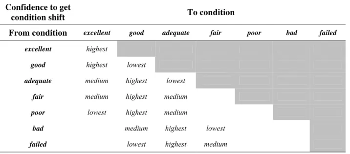
Once the expected post-renewal condition rating and post-renewal deterioration rate factor are computed, the rule-base fuzzy Markov deterioration process (Kleiner et al., 2006) is applied, starting with the condition rating Cr1₆₀, which is taken at the equivalent age τ1. This deterioration process is applied, however, at a slower rate of deterioration compared to the pre-renewal rate. This deterioration ‘slow down’ is achieved by multiplying the deterioration rate at every time step by the factor b1. The resulting pre- and post-renewal deterioration curves are illustrated in

Figure 7. Applying equation (5), it is found that T1 = 38 years, i.e., it is expected that at age (60 +

38 =) 98 the condition of the renewed pipe will be similar to its condition just before renewal. This means that renewal alternative 1 is expected to enable the deference of subsequent renewal by 38 years if none of decision criteria change. If the cost of renewal alternative 1 is say, S1 =

$50,000, the cost per renewal year becomes S1/T1 = $1316. Other renewal alternatives can be

examined in the same manner and if all else remains unchanged, the selected renewal alternative will be the one with the lowest Sk/Tk ratio.

5 Discussion

The research described in this paper and in the companion paper (Kleiner et al., 2006) can be viewed as a first attempt to formalize and standardize a consistent approach to decision-making for buried infrastructure assets such as large-diameter water transmission mains, trunk sewers, etc. The approach consists of collecting, recording and interpreting data, using these data to model and predict deterioration, evaluating failure risk through the pipe life and making rational

decisions on inspection and renewal scheduling. As noted earlier, one of the main problems observed in the course of this research and elsewhere is the severe lack of pertinent data. The adoption of this approach by water utilities will motivate practitioners to collect and record the appropriate data.

Fuzzy techniques were used for this approach because of the capability of these techniques to accommodate data that are uncertain as well as vague and imprecise. The granularities of the various fuzzy sets were taken as seven condition states for pipe condition rating, nine grades for the possibility of failure, nine levels of severity of failure consequences and nine levels of failure risk. However, it should be noted that the mathematical framework of the approach could

accommodate any granularity to suit the user’s preferences.

The proposed method can differentiate between renewal alternatives based on their cost and their longevity. Its current limitations are: (a) assumption that level of service (excluding longevity) is the same for all options, (b) assumption that the cost to implement renewal does not depend on the condition of the asset, and (c) assumption that decision makers will always want to reach maximum risk tolerance (MRT). A recent paper (Kleiner, 2005) expands the proposed method, while addressing two (b and c) of these three limitations

More research is required to formalize a consistent approach to express failure consequences as fuzzy sets. Future availability of data will enable more rigorous case studies. These may be required to better determine the predictive capabilities of the deterioration model as well as to investigate the sensitivities of the model to various assumptions.

6 Summary

The scarcity of data about the deterioration rates of buried infrastructure assets, coupled with the imprecise and often subjective nature of assessment of pipe condition merits the usage of fuzzy techniques to model the deterioration of these assets. The deterioration process is modelled as a fuzzy rule-based non-homogeneous Markov process, in which memberships “flows” from higher to lower condition states. The model is trained using the condition rating(s) of the asset extracted from distress indicators recorded during inspection session(s). The model can be used to predict future deterioration rate of the asset, subject to some judgment-based assumptions. The

deterioration model was partially validated using available data, however, a more rigorous validation is required, with data that have more historical depth as well as consistent inspection techniques.

The prediction of the fuzzy condition rating of the asset is coupled with the fuzzy consequences of failure, using a fuzzy rule base, to obtain the fuzzy risk of failure throughout the life of the asset. This risk of failure is used to make a decision about the scheduling of the next inspection. If renewal action is required, the decision maker uses a structured process to make an educated guess about the performance of the renewal alternatives to be considered. Subsequently, the most economical alternative can be selected.

Acknowledgement

This paper is based on a research project, which was co-sponsored by the American Water Works Association Research Foundation (AwwaRF), the National Research Council of Canada (NRC) and water utilities from the United States and Canada and Australia. The project report, accompanied by a prototype computer application is available from AwwaRF. The project report number is 91087 and its title is “Risk management of large-diameter water transmission mains”.

Notation

bk defuzzified value of BBk. A fuzzy number representing the pipe fuzzy

condition at time step t

Bik (i = 1, 2, …, 5) fuzzy triangular subsets (levels) in the fuzzy set BBk , depicting the fuzzy

deterioration rate of renewal alternative k relative to observed deterioration rate

Ci (i = 1, 2, …, 7) fuzzy triangular subsets (states) in the fuzzy set C, which defines pipe

condition k

tk

C post-renewal condition for renewal alternative k, which was applied at time step tk

k tk

Cs C_tkk immediately before renewal implementation

k tk

Cr k immediately after renewal implementation

tk

C

d0 base deterioration unit

Fi (i = 1, 2, …, 9) fuzzy triangular subsets (levels) in the fuzzy set F, which defines pipe

possibility of failure

Pk (normalized) condition improvement matrix for renewal alternative k

P’k raw condition improvement matrix

Qi (i = 1, 2, …, 9) fuzzy triangular subsets (levels) in the fuzzy set Q, which defines pipe

failure consequences

RZ rule-set governing the risk Z as the function of the fuzzy possibility of

failure F and the fuzzy consequences of failure Q

Τκ time period ‘bought’ by renewal alternative k. The time it will take for the pipe after renewal to reach its pre-renewal condition state

Zi (i = 1, 2, …, 5) fuzzy triangular subsets (levels) in the fuzzy set Z, which defines pipe

risk of failure

zmax maximum risk tolerance

i k

C

τ

μ membership value in condition state (subset) i of the (pre-renewal) fuzzy condition C_τk at time step τ

k

μtAi membership of a pipe to the fuzzy state (subset) Ci at time step t

τk

References

Cromwell, J. E. III, H. Reynolds, N. Pearson Jr., and M. Grant. 2002. Cost of Infrastructure Failure, American Water Works Association Research Foundation, Denver, CO.

Edmonton, City of. 1996. Standard sewer condition rating system report, City of Edmonton Transportation Department, Alberta, Canada.

Guillaumot, V. M., P. L. Dorango-Cohen, and S. M. Madanat. 2003. Adaptive optimization of infrastructure maintenance and inspection decisions under performance model uncertainty, journal of Infrastructure systems, ASCE, 9(4), 133-139.

Hong, H.P. 1998. Reliability based optimal inspection schedule for corroded pipeline,

Proceedings Annual Conference of the Canadian Society for Civil Engineering, Halifax, NS, June, pp. 743-752.

Jiang, M., R.B. Corotis, and J.H. Ellis. 2000. Optimal life-cycle costing with partial observability, Journal of Infrastructure Systems, ASCE, 6(2): 56-66.

Kleiner, Y. 2001. Scheduling inspection and renewal of large infrastructure assets, Journal of

Infrastructure Systems, ASCE, 7(4): 136-143.

Kleiner, Y., Sadiq, R., and Rajani, B. 2006. Modeling the deterioration of buried infrastructure as a fuzzy Markov process. Accepted for publication in Journal of Water Supply: Research. &

Technology-AQUA.

Kleiner, Y. 2005. Risk approach to examine strategies for extending the residual life of large pipes, Proceedings of Middle East Water 2005, 3rd International Exhibition and Conference

for Water Technology, Manama, Bahrain, Nov. 14-16.

Klir, G.J., and Yuan, B. 1995. Fuzzy sets and fuzzy logic - theory and applications, Prentice- Hall, Inc., Englewood Cliffs, NJ, USA.

Lawrence, W.W. 1976. Of acceptable risk, William Kaufmann, Los Altos, CA.

Lee, H.-M. 1996. Applying fuzzy set theory to evaluate the rate of aggregative risk in software development, Fuzzy Sets and Systems, 79: 323-336.

Li, N., L.R. Haas, and W-C. Xie. 1997. Development of a new asphalt pavement performance prediction model, Canadian Journal of Civil Engineering, 24: 547-559.

Li, N., W-C. Xie, and L.R. Haas. 1995. A new application of Markov modelling and dynamic programming in pavement management, Proceedings 2nd International Conference on Road & Airfield Pavement Technology, September, Singapore.

Linstone, H. A. and M. Turoff . 2002. The Delphi method, techniques and applications,

http://www.is.njit.edu/pubs/delphibook/ - an electronic version of the original 1975 book available for free download from the New Jersey Institute of Technology.

Madanat, S.M., and M. Ben Akiva. 1994. Optimal inspection and repair policies for transportation facilities, Transportation Science, 28(1): 55-62.

Mamdani, E.H. 1977. Application of fuzzy logic to approximate reasoning using linguistic systems, Fuzzy Sets and Systems, 26: 1182-1191.

Mendel, J.M. and John, R.I. 2002. Type-2 fuzzy sets made simple, IEEE Transactions on Fuzzy

Systems, 10(2): 117-127.

Pandey, M.D. 1998. Probabilistic models for condition assessment of oil and gas pipelines, NDT

& E International, 31(5): 349-358.

PPK Consultants Pty Ltd. 1993. Identification of Critical Water Supply Assets, Urban Water

Research Association of Australia, Research Report No. 57, Melbourne, Australia.

Rajani, B., Kleiner, Y., and Sadiq, R. 2005. Translation of pipe inspection results into condition rating using fuzzy techniques. Submitted for publication to Journal of Water Supply:

Research. & Technology-AQUA.

WRc 1993. Manual of sewer condition classification, 3rd Edition, Water Research Centre, UK. WRc 1994. Sewer rehabilitation manual, 3rd Edition, Water Research Centre, UK.

Zhao, J. K., and S.E. McDonald. 2000. Development of guidelines for condition assessment and

rehabilitation of large sewers, Client Report (final), National Research Council of Canada, Institute for Research in Construction.

Possibility of failure fuzzy set F Fuzzy subset (F) Qualitative scale TFN representation F1 extremely low (0, 0, 0.125) F2 very low (0, 0.125, 0.25) F3 quite low (0.125, 0.250, 0.375) F4 moderately low (0.250, 0.375, 0.500) F5 medium (0.375, 0. 500, 0.625) F6 moderately high (0. 500, 0.625, 0.750) F7 quite high (0. 625, 0.750, 0.875) F8 very high (0.750, 0.875, 1.000) F9 extremely high (0.875, 1.000, 1.000) 0 1 0 0.125 0.250 0.375 0.500 0.625 0.750 0.875 1

Membership to failed state

0.4 0.6 0 0.1 0.2 0.3 0.4 0.5 0.6 0.7 0.8 0.9 1 0 50 100 150 200 Year M e mb e rsh ip val u e excellent good adequate

fair poor bad

failed moderately high quite high very high extremely high medium Members h ip to F su bsets extremely low very low quite low moderately low

0 20 40 60 80 100 120 140 0 20 40 60 80 100 120 140 Conservative (Upper bound) Optimistic (Lower bound) Defuzzified values extremely high very high quite high moderately high Fuzz y risk l evel medium moderately low quite low very low extremely low Age (years)

109 Next Inspection MLV Conservative Optimistic 0 1 2 3 4 5 6 7 8 9 0 180

Pipe Age (years)

R

isk L

evel

20 40 60 80 100 120 140 160

zmax = moderately high

138

109

bk = 0.944 0 1 Relative value M e m b er sh ip

much lower lower same higher much higher

0.4 0.7 0.1 11 0.8 0.750.9 0.5 1.25_1.1 1.5 _1.2 Fuzzy

subset Qualitative scale TFN representation

BBk 1 much lower (0.50, 0.50, 0.75) BBk 2 lower (0.50, 0.75, 1.00) BBk 3 same (0.75, 1.00, 1.25) BBk 4 higher (1.00, 1.25, 1.50) BBk 5 much higher (1.25, 1.50, 1.50)

0 0.1 0.2 0.3 0.4 0.5 0.6 0.7 0.8 0.9 1 0 20 40 60 80 100 120 140

Pipe Age (years)

M e m b er sh ip t o st at e

Observed data points Inspection 2002 Inspection 1997 Inspection 1999

extremely severe very severe quite severe moderately severe very low quite low moderately low medium Memb ership extremely low 1 A

Figure 6. Example: A - fuzzy consequences. B – life fuzzy risk.

77 0 1 2 3 4 5 6 7 8 9 0 20 40 60 80 100 12 Present time Next inspection 0 Age (years) B Conservative Optimistic MLV Risk level 77 Age (years)

Figure 7. Example: pre- and post-renewal deterioration curves (E = excellent, G = good,

A = adequate, F = fair, P = poor, B = bad).

a P " re-intervention "failed Po " Renew al 98 Next renew al 0.0 0.1 0.2 0.3 0.4 0.5 0.6 0.7 0.8 0.9 1.0 0 20 40 60 80 100 120 140 160

Pipe age (years)

M emb er sh ip val u e Pre-renewal “failed” st-intervention failed" Post-renewal “failed” G E a ‘Time bought’ A F f p b P g E, G,….,B - Pre-renewal states e, g,….,b - Post-renewal states

Table 1. Rule-set RZ for failure possibility-consequence-risk relationship. Failure consequences, Q Failure Possibility, F extremely low very low quite low moderately low medium moderately severe quite severe very severe extremely severe extremely low EL EL VL VL QL QL ML ML M very low EL VL VL QL QL ML M M MH quite low VL VL QL QL ML ML M M MH moderately low QL QL QL ML ML M M MH QH medium QL ML ML ML M M MH MH QH moderately high ML ML ML M M MH MH QH VH quite high ML M M M MH MH QH QH VH very high M M M MH MH QH VH VH EH extremely high M MH MH QH QH VH VH EH EH

EL = extremely low, VL = very low, QL = quite low, ML = moderately low, M = medium, MH = moderately high, QH = quite high, VH = very high, EH = extremely high

Table 2. Expert input for constructing a condition improvement matrix, Pk.

Confidence to get

condition shift To condition

From condition excellent good adequate fair poor bad failed

excellent highest

good highest lowest

adequate medium highest lowest

fair medium highest medium

poor lowest highest medium

bad medium highest lowest

failed lowest highest medium

Table 3. Expert input to evaluate post-renewal deterioration rate, Bk.

Expression of confidence in the post-renewal deterioration rate compared to the current deterioration rate

much lower lower same higher much higher