Modeling the variability of EEG/MEG data through statistical machine learning

(1)

HAL Id: tel-00803958

https://tel.archives-ouvertes.fr/tel-00803958

Submitted on 24 Mar 2013

HAL is a multi-disciplinary open access

archive for the deposit and dissemination of sci-entific research documents, whether they are pub-lished or not. The documents may come from teaching and research institutions in France or abroad, or from public or private research centers.

L’archive ouverte pluridisciplinaire HAL, est destinée au dépôt et à la diffusion de documents scientifiques de niveau recherche, publiés ou non, émanant des établissements d’enseignement et de recherche français ou étrangers, des laboratoires publics ou privés.

Modeling the variability of EEG/MEG data through

statistical machine learning

Wojciech Zaremba

To cite this version:

Wojciech Zaremba. Modeling the variability of EEG/MEG data through statistical machine learning. Computer Vision and Pattern Recognition [cs.CV]. Ecole Polytechnique X, 2012. �tel-00803958�

(2)

École Polytechnique

Faculty of Applied Mathematics

University of Warsaw

Faculty of Mathematics, Informatics and Mechanics

Wojciech Zaremba

Student no. 262981

Modeling the variability of

EEG/MEG data through statistical

machine learning

Master’s thesis in MATHEMATICS First supervisor: Matthew B. Blaschko Assistant Professor

Center for Visual Computing École Centrale Paris

Second supervisor:

Pawan Kumar Mudigonda Assistant Professor

Center for Visual Computing École Centrale Paris

Auxiliary supervisor:

Dr Hab. Hung Son Nguyen Group of Logics

Institute of Mathematics University of Warsaw

(3)

Supervisor’s statement

Hereby I confirm that the submitted thesis was prepared under my supervision and that it fulfils the requirements for the degree of Master in Mathematics.

Date The auxiliary supervisor’s signature

Author’s statement

Hereby I declare that the submitted thesis was prepared by me and none of its contents was obtained by means that are against the law.

The thesis has never before been a subject of any procedure of obtaining an academic degree.

Moreover, I declare that the version of the thesis is identical to the attached elec-tronic version.

(4)

Abstract

Brain neural activity generates electrical discharges, which manifest as electrical and magnetic potentials around the scalp. Those potentials can be registered with magnetoencephalography (MEG) and electroencephalography (EEG) devices. Data acquired by M/EEG is extremely difficult to work with due to the inherent complexity of underlying brain processes and low signal-to-noise ratio (SNR). Machine learning techniques have to be employed in order to reveal the underlying structure of the signal and to understand the brain state. This thesis explores a diverse range of machine learning techniques which model the structure of M/EEG data in order to decode the mental state. It focuses on measuring a subject’s variability and on modeling intrasubject variability. We propose to measure subject variability with a spectral clustering setup. Further, we extend this approach to a unified classification framework based on Laplacian regularized support vector machine (SVM). We solve the issue of intrasubject variability by employing a model with latent variables (based on a latent SVM). Latent variables describe transformations that map samples into a comparable state. We focus mainly on intrasubject experiments to model temporal misalignment.

Keywords

MEG, EEG, brain decoding, mind reading, latent SVM, LSVM, spectral method, laplacian regularization, kernel SVM, event related potential, P300 , BMI, NP-hardness of LSVM

Thesis domain (Socrates-Erasmus subject area codes) 11.0 Mathematics, Computer Science:

11.2 Statistics

11.4 Artificial Intelligence

Subject classification AMS MSC 2000 : 62H12, 62H20, 62H35

(5)

(6)

Introduction

At the end of the XVIII century, Galvani (figure 1.1, [16]) became the first person to register the electrical activity in animal (frog) tissue. His research opened a new avenue of science and paved the way to develop ECG (measures cardiac electrical activity), EMG (for muscle electrical activity) and finally EEG which measures electrical activity of the brain. The first human electrical activity was recorded over a century after Galvani’s discovery by Hans Berger in 1924 [59]. The first recording obtained by Berger is shown in Figure 1.2. Berger’s discovery made it possible to explore human brain activity in a non-invasive manner. Over the years, EEG devices became more and more accurate. Nowadays, they are capable of registering higher temporal and spatial resolution recordings. Another major advance in noninvasive human brain research came in 1968 with David Cohen’s creation of magnetoencephalography (MEG) [21]. The signal registered by this device is complementary to the signal acquired by EEG [60]. Many devices, commonly referred to as M/EEG, simultaneously register both the magnetic and the electrical activity of a patient’s brain.

Figure 1.1: Galvani first discovered the elec-trical properties of animal tissue based on ex-periments performed on frogs (image taken from [49]).

Figure 1.2: The first human EEG record-ing registered by Hans Berger in 1924 (figure from [9]).

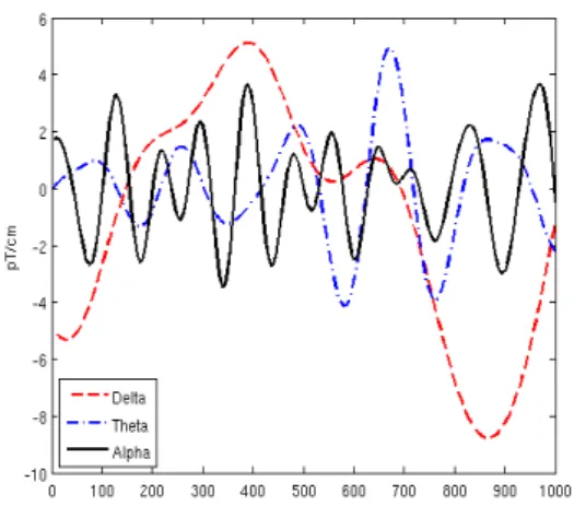
Researchers consider a few frequency bands of brain waves: alpha, beta, gamma, theta, and delta (Figure 1.3 presents some of them) [36]. Different brain activities correspond to different brain wave frequencies. Beta is common during working and alertness states. Alpha is predominant during subject relaxation when a subject keeps his or her eyes closed. A brain generates theta and delta waves during deep sleep. There is no unique correspondence between a task and the frequencies of brainwaves.

In 1964, Chapman and Bragdon conducted research using visual stimuli [19]. They av-eraged the samples resulting from the same stimulus and found that the waves coming from

(9)

Figure 1.3: Frequencies of brain waves. Al-pha waves correspond to concentration and to relaxation states. Theta and delta are present during deep sleep phase.

Figure 1.4: Event related potentials (ERPs) appear after averaging multiple samples be-longing to a single task. ERPs correlate with cognitive tasks like decision making (P300), visual search and attention (P200) etc.

the parietal lobe registered around 300ms after stimuli onset have a distinctive, reproducible shape. Such a cerebrum response is a so called event related potential (ERP), and the afore-mentioned potential has the name P300 (P stands for positive potential, 300 for delay from stimuli onset). Decision making tasks induce a P300 potential. Shortly after their discovery, several other ERPs were identified : early left anterior negativity (ELAN) , N100, N170, N200, P200, and N400 (Figure 1.4). ERPs have a much smaller magnitude in comparison to common brain activity. Averaging multiple samples reveals ERPs. It is not possible to detect ERPs based on a single sample.

Nowadays people use more principled machine learning methods to predict and decode the brain state. This dissertation applies machine learning techniques to determine the similarity of data samples. Chapter 2 describes the problem of cross-subject generalization and presents a measure of similarity between samples based on spectral clustering with a correlation-based measure. Further continuation of this approach is a classification method based on Laplacian regularized SVM (Chapter 3). Chapter 4 focuses on intrasubject classification and provides a method for co-registering samples based on a latent SVM, where the latent variables model the misalignment of the samples. The correct identification of the offset between the samples results in increased prediction accuracy.

1.1. Purpose of brain decoding and reading

M/EEG registers electromagnetic brain activity, which reflects some of the underlying cog-nitive processes. By analysing M/EEG data, neuroscientists attempt to understand how the cerebrum works, and which part of it is responsible for which function [17,35]. This knowl-edge indicates the connection between brain injuries and dysfunctions. It helps to improve clinical rehabilitation methods for afflicted patients.

Another powerful application of M/EEG mind reading is its use as a noninvasive brain computer interface (BCI). BCI are essential for paralyzed patients and locked-in patients to interact with the external world [33,54, 44], for example, to operate a wheelchair or for the

(10)

purposes of communication. The range of BCI applications is not limited to clinical usage. There are publicly available products like Mindball1 _{which measures and purports to improve}

the level of concentration of a subject. Scientists have considered BCI as an interface to pilot an aircraft [2]. There is substantial interest in applying BCI for game control. Pinball is one successfully demonstrated application of a game operated though BCI [56]. There is also the hope that brain decoding allows the reading of emotions [42]. Tan Le, the founder of Emotiv, has suggested that emotions can be used to alter the theme of a game (music, virtual weather etc.). The possibility of retrieving data from the brain has tremendous practical applications.

1.2. Previous work

Common SVM is a popular classifier in neuroscience [6,18]. It does not always provide the best accuracy results because enforcing sparsity often brings higher prediction scores [32]. The brain signal comes from a few aggregated sources, so enforcing sparsity provides knowledge to the classifier that the sources come from a few discrete locations. Sparsity of a signal might be considered in terms of frequency, spacial occurrences, or some spatio-temporal patterns [29,

31]. A common way to enforce sparsity is by applying L1 regularization (the lasso is a name

for this classical setup when squared error is used) [32]. Another avenue is though enforcing sparsity in multiple kernel learning [52].

Univariate statistical mapping analyses are uncommon in M/EEG classification. However, it has yeilded good results in fMRI classification [63]. In fMRI, a classifier matches the observed brain activity against the expected blood-oxygen-level-dependent (BOLD) contrast. Similarity between observed data and the expected BOLD signal gives a single region score. Summed up, thresholded scores make a final prediction.

Common spatial pattern (CSP) is a technique from signal processing to handle non-stationary signals. This mathematical procedure removes any temporal information. It sep-arates a multivariate signal into additive components with the highest difference in variance. CSP is a quite popular technique of M/EEG classification [11,43]. It can be also used in the removal of artifacts.

There are publicly available frameworks for brain data preprocessing, visualization and classification, such as EEGLAB [23], FieldTrip [50], and SPM [26]. Those frameworks focus on signal pre-processing and visualization and offer only elementary suites for data classification. This thesis discusses the issue of subject variability. It approaches it though measuring variability between samples (Chapter 2) and then attempts to use this information for cross subject generalization using a Laplacian regularized SVM. There has been extensive research trying to generalize classifiers for cross subject prediction [58]. However, this task is still difficult. Results described in this thesis show that spectral clustering with a graph based on correlation distance is the most accurate of the evaluated methods in terms of subject discrimination.

Chapter 4 discusses intrasubject variability and establishes the connection with the co-registration problem. It approaches the signal co-co-registration problem though the use of latent SVMs. Latent variables in a latent SVM setup correspond to transformations that adjust samples with respect to each other. Spatial, frequency analysis (Fourier analysis or wavelet analysis) alleviates the problem of intrasubject variability [24,47]. Another approach is to model the nonstationarity of signals [38]. This thesis presents an intrasubject variability model that address the issue of signal misalignment. Such an approach is complementary to spatial analysis, frequency analysis or to nonstationarity modeling.

(11)

1.3. Preliminaries - data acquisition

This section describes some fundamental methods of brain data registration, preprocessing and feature extraction. These processes are essential for any further classification. Although this work is primarily concerned with machine learning techniques, we briefly cover issues of data acquisition here.

M/EEG data acquisition is a quite challenging task. The first step is conducted by a physician or technician who mounts the sensors on a patient’s head. This process involves a soft abrasion of the scalp in order to reduce the impedance conducted by dead skin. The person in charge lubricates the channels with a conductive gel or paste, and mounts the device on the patient’s head. The recordings have to be oversampled, that is, they have to be conducted at a frequency at least twice as high as the expected highest frequency in a signal [48]. The rest of the preprocessing is done in a semiautomatic fashion using specialized software.

1.3.1. Preprocessing

M/EEG measures electrical and magnetic potential on the head surface. However, any elec-trical device can produce an electromagnetic field. This field effects the recordings and gives rise to artifices. Another set of artifices comes from human physiology; it includes heart beat, breathing, eye blinking. The techniques presented in this section helps to cleanse data by removing those unwanted artifices.

The data often contains a few channels and samples with extraordinarily large standard deviation of signal. Those channels and samples are outliers, and corresponding data has to be removed from the dataset. Channels might behave in such a way due a lack of sufficient conductivity (weak lubrication). Some of the samples are useless due to hard to remove artifacts like rapid head movements.

During the early stages of the development of EEG, scientists conducted all studies of brain waves above 25Hz on data acquired in a Faraday cage. A low pass filter is a more convenient remedy for this issue. 50 Hz low pass filter removes the influence of current induction. It turns out that the most of the signal corresponding to cognitive processes lies in the range of 1 to 30 Hz [36]. Signal belonging to those frequencies can be extracted with a combination of a low pass filter and a high pass filter.

Blind signal separation (BSS) is the method of separating mixed signals (usually without a hint about signal source and mixing processes). In M/EEG pre-processing there are two commonly used BSS methods: independent component analysis (ICA) [34] and principal com-ponent analysis (PCA). ICA and PCA are alternative methods in signal processing. However, in M/EEG data processing, researchers use them sequentially. In M/EEG data processing, those methods are complementary, and applying one after another is beneficial.

ICA extracts independent components of a signal. It is a linear transformation such that the dependency between the generated outputs is small. Mutual information or maximization of non-Gaussianity is a common measure of dependency used in ICA. The output generated by ICA on M/EEG data contains a few components that are merely artifacts, like a heart beat or eye blink. The removal of these components is essential for further analysis. There are automatic methods of artifact removal. However, the recording apparatus has to be equipped with additional devices (e.g. electrocardiography - ECG). The component with the highest correlation score with ECG signal is likely to correspond to the heart beat and can be removed. A similar solution exists for eye blink removal using electroretinogram (ERG). It seems that automatic preprocessing of M/EEG signals may be feasible, but it is uncommon

(12)

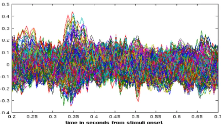
Figure 1.5: A plot of all brain channels averaged over samples for a subject from the LTM dataset. The plot shows the time interval after stimuli onset with all channels super-imposed. Such a plot is refered in literature as a “butterfly” plot [23].

in exploratory research. Methods of automatic component removal are not entirely reliable, and scientists prefer to examine the components manually.

PCA is a common method of dimensionality reduction used in M/EEG preprocessing. It looks for a set of orthogonal vectors in feature space such that data points expressed in this orthogonal basis is maximally linearly uncorrelated. Recordings acquired from multiple channels contain redundant information, due to the nature of the recording process. Channels close to each other record the data belonging to a common brain source. PCA allows the reduction of the dimensionality of data by purging the redundant information shared by several channels.

Channels located in different areas record signals with different magnitude. There is also a severe variation of magnitude between MEG and EEG signals (a few orders of magnitude). Whitening is a method of adjusting the signals from different channels by setting the covari-ance matrix to the identity. Alternative approaches normalize the varicovari-ance per variable.

A specialist conducts the above steps in a semiautomatic fashion. A trained neuroscientist knows what correctly processed cerebrum data looks like after every stage of processing. He or she can identify and remove every artifact manually. Often preprocessing is an iterative method, and an expert has to tune the hyperparameters and to chose the area of intraest manually.

1.3.2. Feature extraction

A commonly used feature in M/EEG brain decoding is just an average of values over an interval [23]. ERPs are a manifestation of postsynaptic activity, and often scientists consider an average over time series as bulk information about postsynaptic activity. Theoretically, averaging should remove noise and preserve the desired potential. Researchers use other fea-tures based on statistics like the slope of a fitted line, detrended variance, detrended standard deviation, detrended skewness, detrended kurtosis, variance, standard deviation, skewness, kurtosis, and fluctuation around the mean [32]. Spatio-frequency based statistics are another commonly used set of features. Among them, popular features are coefficients of the Fourier transform (or windowed Fourier transform), or coefficients of a Gabor transform [23]. Zhang et al. [64] explore more exotic wavelet transforms such as second-order Symlet wavelet. Spe-cialists examine the spectrum of wavelet transforms visually, and they choose the frequency and temporal areas with the highest average response. A common way to inspect the data is

(13)

to visualize a so called “butterfly” plot (Figure 1.5). It is the plot of super-imposed averaged signals from all channels.

To date, there is no unified theory which would explain how to choose features in M/EEG analysis. It is often unclear which features are complementary and which are alternative. One approach is to simply consider a large number of features. However, it often hinders prediction, due to the statistical risk caused by the resulting dimensionality explosion. Huttunen et al. [32] explore the issue of feature selection for M/EEG inference. They propose to use various greedy algorithms. Only in some isolated cases is there a guarantee that the selected features will not be redundant (e.g. when features come from a projection to an orthogonal basis [64]).

1.4. Data collection and experimental paradigm

This study employs two data sets. The first dataset explores the process of long memory retrieval. The second dataset is involved with explaining the encoding of artificial and nonar-tificial objects in the brain. We refer to those experiments under acronyms LTM (long term memory) and AVNA (artificial-vs-non-artificial). Both the datasets are publicly available.2

The public datasets for AVNA and LTM contain only two subjects (instead of 11 originally published in the case of LTM [6] and nine in the case of AVNA [18]). The following description has been taken from the original publications associated with the datasets.

LTM dataset

A total of 11 right-handed volunteers (5 male), with a mean age of 23.69 years (SD = 4.64), were recruited amongst university students and employees. Eligible subjects were proficient in Dutch or English, did not have any neurological or psychiatric history, were not colorblind and had adequate eyesight to perform the task. Additionally, we prescreened for any irremovable metal objects attached to the subject’s body. In order to prevent language specific effects, we only included subjects with a Latin alphabet-based native writing system. Native language of the final 11 subjects was Dutch (5), German (4), English (1) and Swedish (1). Prior to starting any experimental procedures, we obtained written informed con-sent of the subject. All subjects were paid for their participation. Experimen-tal procedures were in accordance with the Declaration of Helsinki (Edinburgh Amendments) and approved by the designated ethical committee (CMO commit-tee on Research Involving Humans, region Arnhem-Nijmegen, the Netherlands). MEG recordings we acquired electrophysiological data using a 275-sensor axial gradiometer MEG system (VSM MedTech Ltd., CTF Systems, Coquitlam, BC, Canada), located in a magnetically shielded room. With one sensor being de-fective, we successfully recorded data from only 274 sensors. Data was low-pass filtered at 300 Hz and digitized at 1200 Hz. We attached localizer coils to the subject’s nasion and both ear canals, in order to monitor head position related to the gradiometer array. Additionally, we obtained vertical (VEOG) and horizon-tal electrooculograms (HEOG), using bipolar electrodes mounted on the suborbit and supraorbit of the subject’s left eye and external canthi of both eyes, and an electrocardiogram (ECG), by attaching an electrode below the subjects’ left clav-icle and one on the left lower rib cage. To ensure a sufficiently noise-free signal, 2_{http://www.biomag2012.org/content/data-analysis-competition}

(14)

impedance of the electrooculogram electrodes was reduced to a value below 10 kΩ before recording commenced. [6]

AVNA dataset

Nine right-handed, healthy male volunteers were recorded using simultaneous scalp EEG and MEG while performing auditory and visual versions of a language task. The two tasks were performed in two separate sessions, separated by an average of 4 months. Participants were native-English speakers between the ages of 22– 30. This study was approved by the local institutional review board, and signed statements of consent were obtained from all subjects.

MEG was recorded using a 306-channel Elekta Neuromag Vectorview system (Stockholm, Sweden). Signals were digitized at 600 Hz and filtered from 0.1 to 200 Hz. Data from magnetometers and gradiometers were recorded, however only gradiometers were utilized in this study due to the lower noise in these sensors. Simultaneous EEG recordings were obtained from a 64-channel EEG cap at a sam-pling rate of 600 Hz with the same filter settings as the MEG recordings. EEG was recorded using a mastoid electrode reference but were converted to a bipolar montage to reduce noise. [18]

Figure 1.6: This figure presents the task that subject performed during the LTM experiment. An image of an object appears during the first 200ms of presentation (also called stimuli onset). Then there is a two second pause to associate the object to the color and slope of stripes. Randomly colored and oriented stripes appear for the next 200ms. The subject has to decide if the presented color and angle is the one which corresponds to the object (figure from [6]).

In the LTM experiment, researchers for experimental purposes have established a rela-tionship between a set of objects and colors (red or green) and slope of stripes (45◦_{, 135}◦

degree). For instance, the teddy bear object is paired with the color green and 45◦ degree stripes. Subjects had to memorize this relationship prior to the LTM experiment. The task of a subject is to recall the color and direction of stripes related to an object. Figure 1.6 presents the task paradigm. An image of an object pops up during the first 200ms, and this point is when the stimuli onset is defined to start. Then there is a two second pause to recall the object color and grating. A random color and grating appears for the next 200ms. The subject has to decide if the presented color and grating corresponds to that associated with the object. The dataset contains only correct responses from the subjects, and the number of acceptances and rejections is equal. Half of the time during experimental evaluation, a correct answer is to reject the presented color and grating. The goal of the LTM experiment is to elucidate temporal dynamics of long term memory encoding.

(15)

We employ the AVNA and LTM datasets in the subject clustering experiments discussed in Section 2.3 (only resting state of subjects). We use the LTM dataset in the two other classification experiments discussed in Sections 3.3 and 4.3. In the classification settings, we only predict color (not a grating). It simplifies the setup to a binary classification problem. In all setups, datasets were balanced; there was always an equal number of samples belonging to each considered class.

(16)

Chapter 2

Clustering

Cross-subject M/EEG signal classification is much more challenging than intrasubject clas-sification. In various classification studies [18], people have noticed a significant decline in accuracy as multi-subject data was employed. It seems that even if cross-subject data contains more samples, those additional samples, instead of helping, rather confuse the classifier and reduce the accuracy of classification. A common explanation is that there is a tremendous variation between M/EEG signals among subjects and M/EEG data has low SNR. Human brains and human brain responses significantly differ among individuals.

This study provides an answer to the question of how diverse is multi-subject M/EEG data. Understanding what distinguishes different subjects might allow the generalization of classifiers for cross subject studies. The degree of similarity between subjects could potentially indicate when and if it is possible to generalize a classifier. In the next chapter (Chapter 3), we unify a notion of clustering with classificaiton in a joint learning framework (Laplacian regularized SVM).

The rest of this chapter is organized as follows. Section 2.1, which is concerned with k-means, and Section 2.2, which covers spectral clustering, discuss the theory of commonly used clustering methods. The final result Section 2.3 presents an evaluation of the application of these clustering methods to M/EEG data. Chapter 3 is a natural continuation of the spectral clustering topic, where we try to retain clustering information in unified classification settings based on a Laplacian regularized SVM.

2.1. k-means

k-means is one of the most popular clustering algorithms. Its objective function is the following: min S,µ k X i=1 X j∈Si d(xj, µi)2 (2.1)

S = {S1, . . . , Sk} denotes a data partition and µ1, . . . , µk denotes the cluster centers. d

is an arbitrary distance function, e.g. Euclidean distance, correlation distance, Hamming distance, etc. Finding the global minimum of the k-means objective function is a NP-hard problem [4]. Instead of looking for the global minimum, the standard optimization algorithm returns a local minimum (which in many cases is a reasonable solution) [30]. Optimization is an iterative procedure which alternates between (i) finding the best partition S based on µ

(17)

Algorithm 1 k-means algorithm

Input: Input points {x1, . . . , xn}, number of clusters k, distance measure d : X × X → R

Output: Partition S = {S1, . . . , Sk}

Initialize S with random cluster assignment repeat for i=1:k do µi ← arg minµ P j∈Sid(µ, xj) 2 end for for i=1:k do Si ← ∅ end for for i=1:n do j← arg min d(µj, xi) Sj add element i end for until convergence

and (ii) recalculating µ based on the newly assigned partition S, and is commonly derived as a special case of expectation propagation (EM) [10]. Algorithm (1) describes the optimization procedure. It is worth pointing out that the final result highly depends on the distance function and on initialization (various initializations give rise to various local minima of the optimization objective). Often, optimization consists of several executions of the k-means algorithm with random initialization. The result giving the lowest objective value is taken as the output.

2.2. Spectral clustering

Let us consider an undirected, weighted graph G = (E, V ) with weights {wi,j}i=1,2,...,n;j=1,2,...,n.

Points v ∈ V of this graph represents input data, and weight wi,j of an edge (vi, vj) = e ∈ E

is a similarity between input points xi and xj. There are a few commonly considered

con-structions of the weights wi,j:

k-nearest neighbors graph

wi,j =

(

1, i belongs to the k-nearest neighbors of the vertex j with respect to distance d 0, otherwise (2.2) ε-neighborhood graph wi,j = ( 1, d(i, j) < ε 0, otherwise (2.3)

(18)

fully connected graph

wi,j = exp−

d(i,j)2

2σ2 (2.4)

Let us denote the degree of the vertex vi by di. The volume vol for a set of vertices A and

distance between sets of vertices W (A, B) is defined as follows: di= X (i,j)∈E wi,j vol(A) =X i∈A di W(A, B) = X i∈A,j∈B wi,j (2.5)

Clustering of input points x1, x2, . . . , xn can be expressed in terms of partitioning vertices

of the graph G. Partitioning the graph can be expressed as the minimization of the objective functions RatioCut or N Cut defined as follows [57]:

RatioCut(S1, . . . , Sk) = 1 2 k X i=1 W(Si, ¯Si) |Si| N Cut(S1, . . . , Sk) = 1 2 k X i=1 W(Si, ¯Si) vol(Si) (2.6)

RatioCutencourages the splitting of a graph into subsets of vertices such that there is a small number of connections between sets (S1, S2, . . . , Sn) (W (Si, ¯Si) is small). N Cut similarly

tends to have a small value of W (Si, ¯Si). The only difference between RatioCut and N Cut

is the normalization of the term W (Si, ¯Si). In both cases the value W (Si, ¯Si) is divided by

the set size Si, however for RatioCut, the size is defined as |Si| and for N Cut it is vol(Si).

The objective functions for these problems are defined as follows:

min S={S1,...,Sn} RatioCut(S1, . . . , Sk) or min S={S1,...,Sn} N Cut(S1, . . . , Sk) (2.7)

These objectives can not in general be minimized exactly in polynomial time (finding the op-timal balanced cut of an undirected weighted graph is a NP-hard problem). An approximate solution to the n-clusters clustering problem RatioCut corresponds to clustering n eigenvec-tors (starting from the second smallest eigenvector) of the unnormalized Laplacian operator

(19)

Figure 2.1: This figure presents samples from a swiss roll distribution. The distance on the swiss roll manifold significantly differs from common distance measures (Figure from Stéphane Lafon et al. (2006) [41]).

which is defined as follows:

D= diag(d1, d2, . . . , dn)

W = {wi,j}i=1,...,n;j=1,...,n

L= D − W

(2.8)

N Cut similarly to RatioCut defines a Laplacian operator, however its definition slightly differs: Lsym= I − D− 1 2W D− 1 2 (2.9) The optimization procedure for spectral clustering with an unnormalized Laplacian oper-ator is described in detail in Algorithm 2.

Algorithm 2 spectral clustering algorithm for unnormalized Laplacian operator Input: Graph edge weights W , number of clusters k

Output: Partition S = {S1, . . . , Sk} for i=1:n do di ←P_(i,j)∈Ewi,j end for D← diag(d1, d2, . . . , dn) L← D − W

v0, v1, v2, . . . , vk← smallest k + 1 eigenvalues of the matrix L

S← k-means(v1, . . . , vk) where k-means is described in Algorithm 1

2.3. Results

We have executed all clustering experiments on the common datasets: LTM and AVNA. These datasets are described in more detail in Section 1.4. In the case of AVNA data, we consider four different inputs for the experiment: (i) MEG signal, (ii) EEG signal, (iii) M/EEG signal

(20)

Figure 2.2: A plot of all brain channels for two subjects during resting state. Each plot is a single sample of a single subject with all channels super-imposed.

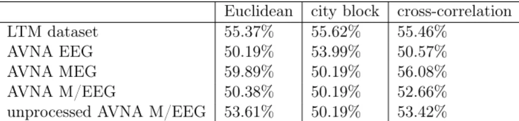
Euclidean city block cross-correlation

LTM dataset 55.37% 55.62% 55.46%

AVNA EEG 50.19% 53.99% 50.57%

AVNA MEG 59.89% 50.19% 56.08%

AVNA M/EEG 50.38% 50.19% 52.66%

unprocessed AVNA M/EEG 53.61% 50.19% 53.42%

Table 2.1: Accuracy of k-means clustering of subjects with various distance measures.

(iv) data before ICA processing (after bandpass filtering). We have performed the LTM exper-iments on the fully preprocessed MEG data. We have coalesced 200ms recordings of resting state belonging to two subjects performing the same experiment on the same recording device. The task is to recover subjects from the mixed data. It can be stated as a clustering task were clusters correspond to subjects. In these studies, we considered the k-means algorithm with different distance measures and spectral clustering methods. Table 2.1 presents results of the k-means algorithm applied with different measures for clustering. It gives rather weak accuracy (50% accuracy corresponds to chance performance). This is supported by Figure 2.2 as there is little visible structure that distinguishes subjects. Poor accuracy results of k-means clustering indicates that data acquired from different subjects is not trivially separable. In many setups, Euclidean distance is the best choice [3]. However, in the case of the subject separation problem it fails severely (Table 2.1).

Next we have performed an equivalent experiment using the spectral clustering framework. The graph used for spectral clustering was created as an adjacency graph based on 6-nearest

Euclidean city block cross-correlation

LTM dataset 54.23% 54.64% 91.69%

AVNA EEG 51.52% 89.35% 95.25%

AVNA MEG 51.71% 50.19% 99.62%

AVNA M/EEG 56.84% 53.23% 99.81%

unprocessed AVNA M/EEG 50.19% 50.95% 52.85%

(21)

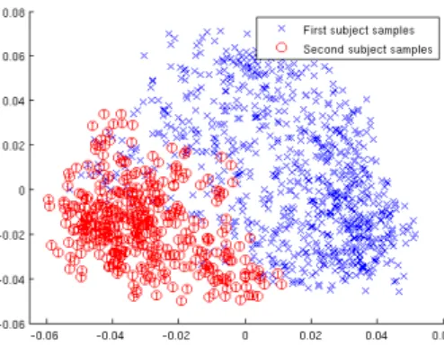
Figure 2.3: Spectral clustering of subjects for the LTM dataset

neighbors based on different distance measures. We used a normalized Laplacian and the final k-means clustering step (c.f. Algorithm 2) was executed on three eigenvectors (second, third and fourth smallest). Table 2.2 presents clustering accuracy results. Subject recovery with spectral clustering for correlation measure gives very high accuracy scores and significantly outperforms the k-means algorithm. The first two dimensions of the Laplacian eigenmap [7] are visualized in Figure 2.3.

Gramfort et al. [28] have conducted research about the relative displacement of samples. Their studies are based on single subject data. They have shown that the second smallest eigenvector of spectral Laplacian (also known as the Fiedler vector [25]) indicates the relative order of samples. Our study indicates that larger eigenvectors have high discriminative power in terms of subject diversity in multi-subject experiments.

(22)

Chapter 3

Laplacian regularization

Due to the high diversity between subjects, it is quite difficult to generalize a learning approach to a cross-subject setting. Based on the great discriminative power of spectral clustering in terms of subject classification (presented in Chapter 2) we have investigated Laplacian regu-larized SVM. The following sections give an overview of a SVM and its Laplacian reguregu-larized variant [5]. The final section (Section 3.3) presents classification results for various setups of the Laplacian regularized SVM.

3.1. SVM

Notation Let the input be denoted by x ∈ X, the output by y ∈ Y = {−1, 1}. The training dataset D = {(xi, yi)}i=1,...,n consists of n input-output pairs (samples). φ(x) is a feature

vector of the input variable.

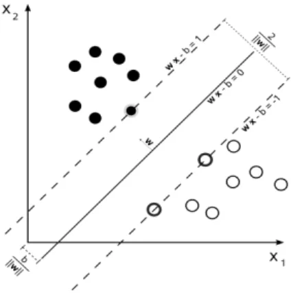
The support vector machine (SVM) is a popular classification method introduced by Cortes and Vapnik [22]. Its simplicity and flexibility together with good prediction results make it one of the most popular classification methods. A SVM looks for the surface w which separates points φ(xi) in the feature space with the highest margin (Figure 3.1). The objective function

also minimizes the sum of the slack variables ξi, and a small value of the slack variable

results in the correct classification of a training data point. The regularization term kwk2

in the objective function prevents overfitting. The multiplier, C, is a trade-off parameter

Figure 3.1: SVM looks for a prediction function, w, that maximizes the margin between classes. The distance between the separating hyperplane and the closest points (support vectors) is equal to _||w||1 (image source Wikimedia).

(23)

Figure 3.2: A kernelized SVM can have a non-linear prediction boundary (source Wikimedia). between the regularization and the misclassification error. The SVM objective is stated in Equation (3.1). min w,ξ 1 2kwk 2_+CX i ξi yiw⊤φ(xi) ≥ 1 − ξi ξi ≥ 0 (3.1)

The SVM formulation (3.1) is a quadratic programming problem, which implies the existence of a unique, global minimum, which can be easily computed numerically.

Often SVM optimization is formulated in the Lagrange dual form. The Karush-Kuhn-Tucker conditions re-prove the representer theorem [37, 53] for the special case of the SVM. Problem 3.1 is a convex optimization problem and it fulfills Slater’s condition [15]. It implies that the optimal dual objective results in the same optimal value as the primal objective. The Lagrange dual formulation to the standard SVM is as follows:

max α X i αi− 1 2 X i X j αiαjyiyjφ(xi)⊤φ(xj) αi ≥ 0 αi≤ C (3.2)

The term φ(xi)⊤φ(xj) is a dot product between vectors φ(xi) and φ(xj). It can be replaced

by any arbitrary dot product k(xi, xj). Replacing φ(xi)⊤φ(xj) with k(xi, xj) is often referred

to in the literature as the “kernel trick” [1]. The “kernel trick” allows the computation of a SVM for elements which do not belong to a Euclidean space, e.g. graphs or trees. It is sufficient to define the dot product k(·, ·) between elements of the input space. The “kernel trick” allows the introduction of a non-linear prediction boundary through the use of a non-linear inner product (Figure 3.2).

Mercer’s theorem states that any function k(·, ·) that is positive semi-definite symmetric can be written as hφ(xi), φ(xj)iHfor some φ that maps to a Hilbert space, H. The mapping,

(24)

mapping of data points to high-dimensional spaces or even to infinite-dimensional spaces for which φ cannot be explicitly computed. For instance, a Gaussian kernel, k(a, b) = eka−bk22σ2 , turns out to give rise to an infinite-dimensional mapping.

3.2. Theory of the Laplacian Regularized SVM

Laplacian Regularized SVM is a semi-supervised learning method that generalizes the stan-dard SVM [8]. The only difference in comparison to a conventional SVM is an additional regularization term, ||w||L, in the objective function. The term ||w||Lensures that the

predic-tion boundary passes through an area of low density on the data manifold, which is estimated non-parametrically. Formally, Laplacian regularized SVM is stated as follows in Equation 3.3.

min w,ξ 1 2kwk 2_+γkwk L+ C X i ξi yiw⊤φ(xi) ≥ 1 − ξi ξi ≥ 0 (3.3)

The estimate of the data manifold is implicit in the graph Laplacian employed in this regu-larization, e.g. by employing the Laplacian defined in Equation (2.9).

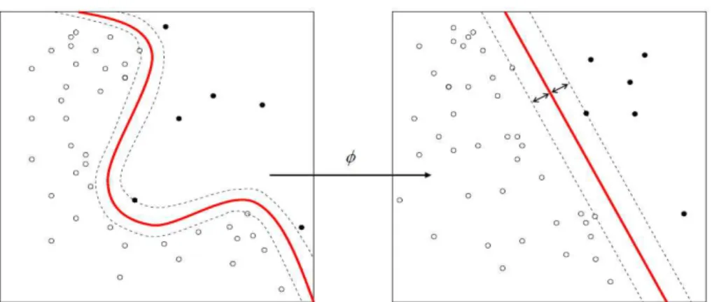
Let us consider the situation presented in Figure 3.3, where a red circle corresponds to a sample of one class, a blue diamond to a sample of another, and black circles are unlabeled data points. Supervised settings such as SVM, univariate Bayesian inferrence, etc., would generate a straight line prediction boundary as is depicted in the left of Figure 3.3. However, based on the unlabeled data marked as small black circles in right side of Figure 3.3 we can expect that a much better choice is a circular boundary as it passes through an area of low density on the data manifold. It has been shown recently that Laplacian regularization has improved classification in a fMRI setting [12,14], however it remains to be seen whether this result generalizes to M/EEG. We explore this question empirically in the next section.

Figure 3.3: Laplacian regularization setup. The red ball and blue diamond belong to different classes. Small, black circles indicate unlabeled data. (i) The left picture presents the predic-tion boundary according to a convenpredic-tional SVM. (ii) The right picture shows the predicpredic-tion boundary according to a Laplacian regularized SVM. (Figures from Belkin et al. (2006) [8])

(25)

3.3. Results

In these experiments, the Laplacian was estimated from both training and testing data (i.e. a transductive learning setting). The Laplacian employed was computed using the cross-correlation distance with a k-nearest neighbor graph as in Section 2.3.

Based on the results described in Section 2.3 we know that the graph based on the corre-lation measure gives rise to a manifold estimate that separates subjects. In this experiment we would like to use this knowledge to generalize to cross-subject prediction. The goal is to establish a single learning framework for cross-subject classification that gives a similar level of accuracy as classification performed on each of the subjects separately. We expected that the Laplacian regularizated SVM will allow the generalization over subjects and that the regularization term would effectively separate subjects. To our surprise we were not able to recover the average accuracy from separate classifiers in a single Laplacian regularized setup. Our hypothesis was that a Gaussian kernel would be able to learn a sufficiently general clas-sification function, because it can have a non-linear prediction boundary. Table 3.1 presents accuracy results. This table consists of results for the first subject, the second subject, and classification for both subjects together. “Separate prediction” was achieved by a weighted average of prediction scores for separate classifiers trained on individual subjects, proportional to the number of samples for that subject. Table 3.1 shows classification results for both the linear kernel and the RBF kernel.

Kernel type Subjects Laplacian SVM SVM

first subject 63.43% 63.28%

Linear kernel second subject 57.92% 56.79%

together 56.61% 57.96%

separate prediction 61.00% 60.42%

first subject 63.12% 62.03%

RBF kernel second subject 57.92% 54.15%

together 55.93% 57.96%

separate prediction 60.83% 58.56%

Table 3.1: Accuracy for cross-subject prediction with and without Laplacian regularization. We expected that Laplacian regularized SVM can achieve the same accuracy with a Gaussian (RBF) kernel (where the prediction boundary is not linear) as the averaged score of the classifiers on the subject separated data. However Table 3.1 shows that the result 55.93% (RBF kernel for mixed subjects) is smaller than 60.83% (RBF kernel for separate subjects). Furthermore, a SVM without Laplacian regularization gave slightly better accuracy (the result without Laplacian regularization for mixed data with a RBF kernel is 57.96%, Table 3.1). It is not clear whether Laplacian regularization is harmful in general in this setting, or whether we simply had an insufficient sample to accurately estimate the Laplacian.

(26)

Chapter 4

Modeling data distortions

One of the main difficulties that we face when working with EEG and MEG data is the variability among the samples collected from the same experiment [20]. The factors for the variability are many folds: level of concentration, vigilance, or familiarly with the experimental setup. As the aforementioned factors are beyond the control of the person conducting the experiment, intra-sample variability is an inevitable artifact of using EEG/MEG data that hinders the prediction procedure. Additionally many mental components P300, P3a, P3b, P2 appear in a highly similar time frame and can be easily confused [51]. To alleviate this problem, we propose a latent variable model, where the latent variables corresponding to a sample represent the variability of the sample. We model variability explicitly, which allows us to more easily compare samples. In order to learn a classifier in the presence of latent variables, we rely on the latent SVM framework. The results section shows that this approach provides a significant improvement in the prediction accuracy over a baseline method that does not explicitly model the sample transformation.

The remaining chapter is organized as follows. In the next section, 4.1, we describe the general latent SVM formulation. In Section 4.2, we show how we can model the distortions in EEG and MEG data using latent SVM. Finally, in Section 4.3, we present empirical results using a large, publicly available dataset.

4.1. Theory of latent SVM

Notation Let the input be denoted by x ∈ X, the output by y ∈ Y , and the latent variables by h∈ H. The training dataset D = {(xi, yi)}i=1,...,n consists of n input-output pairs (samples).

The joint feature vector of the input x and the latent variable h is denoted by φ(x, h). Latent SVM (LSVM) [61] is an extension of the SVM framework, and it relies on the un-derlying assumption that there is a hidden variable which describes the dependency between input points and output values. Knowledge of the latent variable should help in the classifi-cation process. A typical appliclassifi-cation of latent SVM is object recognition, where the loclassifi-cation of object in an image is unknown [46,13,39]. Such an approach models the bounding box of the object as a latent variable. Finding the bounding box that contains the object of interest significantly increases the classification accuracy. For the sake of simplicity, we restrict our description to a binary latent SVM. However, we note that more general structured output latent SVMs also exist in the literature [61]. Formally, the parameters w of a latent SVM are obtained using the following optimization problem:

(27)

min w,ξ 1 2kwk 2₊X i ξi max h yiw ⊤_φ(x i, h) − max ˆ h ˆ yw⊤φ(xi, ˆh) ≥ 1 − ξi ξi≥ 0, ˆy6= y, ˆh ∈ H (4.1)

Similar to the non-latent SVM (c.f. Section 3.1), the regularization term kwk2 _{in the}

objec-tive function helps to avoid overfitting. In addition, the objecobjec-tive function also minimizes the sum of the slack variables ξi, one for each sample (xi, yi). A small value of the slack

variable results in the correct classification of a training sample (in other words, it minimizes the misclassification error over the training data). The constraints stated in equation (4.1) encourages the best latent variable for the correct output to have a score that is greater than all other scores.

The main disadvantage of the LSVM optimization problem is its non-convexity. There does not exist an optimization algorithm that would guarantee convergence to a global minimum in polynomial time. We present a proof showing that the above optimization problem is NP-hard in Appendix A. In this chapter, we focus on a specific instance of latent SVM (Section 4.3), and Appendix B contains proof that this specific case is an NP-hard problem.

The above problem is a difference-of-convex optimization program. This observation sug-gests that a local minimum or saddle point solution for LSVM can be obtained using the concave-convex procedure (CCCP) [62,61]. The first step of the algorithm imputes the best value of the latent variables for all samples using the current estimate of the parameters. In the next step, the imputed latent variables are kept fixed, and the parameter is updated by solving the resulting convex optimization problem.

Algorithm 3 Latent SVM optimization procedure

Input: (x1, y1), (x2, y2), . . . , (xn, yn) data points with ground truth labels. Function φ : X ×

H→ H jointly maps input with latent variables to the feature space. Output: Prediction function w

for i=1:n do

hi ← random element from H

end for repeat

w← Solve QP Problem 4.1 for the input (x1, h1, y1), (x2, h2, y2), . . . , (xn, hn, yn)

for i=1:n do

hi← arg maxhyiw⊤φ(xi, h)

end for

until convergence

There is a guarantee that the objective of LSVM decreases over iterations, and since the objective is bounded from below by 0, it implies that the algorithm would eventually con-verge [55].

There is a danger that the optimization algorithm, 3, will get stuck in a local minimum and might give poor predictions results. A pragmatic solution to this problem is to initiate the algorithm multiple times with different starting values of the latent variable. The parameter that provides the lowest objective function can then be retained as the final solution. There are a few other, more principled, alternatives to alleviate the problem of inaccurate local

(28)

Figure 4.1: Figure presents two samples over a time and visualizes issue of misalignment for M/EEG data. In order to compare samples, first we have to shift them with respect to each other.

minima [45,40]. However none of them thoroughly resolves this issue, because, as mentioned previously, it is an NP-hard problem (more details in Appendices A and B).

4.2. Distortion model

We now describe how the LSVM formulation can be used to handle the transformations in EEG and MEG data. In this case, H is the space of all possible transformations that an EEG or MEG signal undergoes during data acquisition. For example, H can vary from a simple translation of the signal to a more complex affine transformation or to warping (which allows us to model multiple source misalignments). For an input x and a latent variable h ∈ H, we denote the feature map of the resulting transformed signal as φ(x, h). Given a training dataset D = {(xi, yi)}i=1,...,n, our goal is to learn a classifier that is not only able to predict

the output yi accurately, but is also able to predict the correct transformation hi for each

sample.

We consider a simple distortion model where samples are shifted with respect to each other (H contains a fininte set of translations). This latent variable model uses a putative offset to describe the misalignment, and φ(x, h) is defined as follows:

x= (a1, a2, . . . , an)⊤

φ(x, h) = (as+h, as+1+h, . . . , al+h)⊤,

1 ≤ s + h ≤ s + l + h ≤ n

(4.2)

where s to l is a range over which we consider the signal to be informative (1 to n is a range of entire signal). For H = {c}, for any constant c, this instance of latent SVM simplifies to the standard SVM formulation.

(29)

Figure 4.2: Visualization of the linear classifier of the LTM dataset. Red regions indicate putatively responsible brain regions for the long term memory association process. Blue regions correspond to non-discriminative regions in terms of the LTM memory association. The number displayed above the braim map indicates time passed from the stimuli onset.

Figure 4.3: Results of a latent SVM for the LTM dataset where the latent variable mod-els misalignment

Figure 4.4: Offset imputed on samples in la-tent SVM where the lala-tent variable models misalignment

4.3. Results

To test the efficacy of LSVM, we performed our experiments on the LTM dataset (described in detail in Section 1.4). Recall that, in the LTM dataset, the task is to predict the color retrieved from a subject’s memory. It is a case of a binary classification problem. We have visualized the weights resulting from a binary SVM in Figure 4.2. We considered a distortion model where the latent space H consists of a finite number of translations. Figure 4.3 presents the accuracy results for various sizes of the latent space. The point denoted by 10 in the x-axis denotes the experiment where the putative translation is restricted to lie in the interval [−10ms, 10ms]. For computational efficiency, we discretized the space of putative translations into 7 equally spaced values, resulting in the latent space H = [−3, −2, −1, 0, 1, 2, 3] (the data acquisition rate is 300Hz). For the sake of brevity, we refer to latent SVM setup with considered misalignment N ms under the alias M isAlignN.

The results presented in Figure 4.3 are cross-validated over the trade-off parameter C be-tween the regularization and the misclassification error. The accuracy obtained for M isAlign10

is 2.19% higher compared to the accuracy obtained by a standard SVM. The accuracy peaks when we consider the misalignment to lie in the interval [−10ms, 10ms] and it slowly decays for bigger values of misalignment. Our experiments indicate that the misplacement of most of the samples is up to 10ms and considering higher values of misalignment confuses the classifier (for the majority of samples higher values do not correspond to actual data misalignment).

(30)

Cross validation over the size of the latent space increases the accuracy gap over the con-ventional SVM to 2.97%. There is a large standard deviation in the accuracy results; it is 3.62% for a common SVM. M isAlign10 gives a higher score for every fold in comparison to

a typical SVM. A paired t-test indicates that the M isAlign10 distribution is different from

the accuracy distribution obtained for a standard SVM. We evaluate the paired t-test with accuracy results obtained from 5-fold cross validation. A paired student’s t-test rejects the null hypothesis with p-value equal to 4.47% (rejection of the null hypothesis is accepted for p below 5%). Accuracy scores for the setup where the size of the latent space H is cross validated further reduce the probability of the null hypothesis (p = 3.76%). The low value for the probability of the null hypothesis indicates that the improvements obtained by the latent SVM formulation are statistically significant.

The imputed latent variables provide further empirical evidence for the importance of modeling the data misalignment. Latent SVM has the freedom to choose all latent variables to be constant (samples with the same shift offset are not relatively misplaced). However, as Figure 4.4 shows, the imputed latent variables are not the same for more than 20% of the samples for any putative value.

(31)

(32)

Chapter 5

Discussion

The results presented in Section 2.3 show that spectral clustering based on correlation distance is the most powerful method in terms of subject clustering. Any other clustering method and distance measure does not provide such a high score. The failure of k-means clustering for every considered measure indicates that data points are not easily distinguishable. k-means gives poor results even using the correlation distance measure. Gramfort et al. have shown that the first eigenvector of the Laplacian constructed using the correlation measure (spectral clustering relies on clustering eigenvectors of the Laplacian operator) gives an order of samples corresponding to their misalignment offset [28]. Our findings (Section 2.3) and those of Gramfort et al. suggest that brain waves for a single subject are more aligned with respect to each other than across subjects. This intuition is a key motivation to consider a latent SVM setup, which models explicitly the variability of samples. It might be necessary to model a much richer family of transformations to co-register cross-subject data. The location of the signal in the brain and signal onset may vary over subjects.

We attempt to utilize results from spectral clustering in the single classification setup. The approach presented in the results section (Section 3.3) seems to fail. Both linear and non-linear (RBF kernel) prediction functions give poor accuracy and do not generalize to cross-subject classification. A Laplacian regularizer encourages the prediction boundary to pass through an area of low density along the data manifold. We had hypothesized that a non-linear classifier with Laplacian regularization may be able to learn a function that has largely differing values across subjects, which implies effectively different functions along each of the subject’s submanifolds. We have expected that the prediction boundary would pass freely through areas which separate subjects. A joint learning framework is highly desirable in order to begin to enforce cross-subject generalization. We still expect that generalization can be achieved (maybe in a setup with a different non-linear kernel). Extremely high clus-tering accuracy makes us believe that spectral clusclus-tering can be generalized to a cross-subject classification setup.

The results presented in Section 4.3 provide an estimate of the misalignment between samples. It indicates that aligning samples up to 10 ms increases significantly the prediction accuracy. There are various possible explanations why aligning samples increases accuracy. We consider a few theories that may explain the empirical results:

• Brain responses may have varying delays as a result of subject tension, concentration, vigilance and familiarity with the experiment. Latent SVMs model those parameters and align all samples to a common template, where it is easier to compare them with each other. That is our primary motivation to use a latent SVM.

(33)

• Stimuli onset is not clearly defined, and latent SVM aligns samples to a common stimuli onset. This explanation fits partially into the realm of the previous explanation. How-ever, if it is the only cause of the superiority of latent SVM over a standard SVM then there is no point to consider more complex transformations such as affine transforma-tions or warping.

• Latent SVM aligns ridges of non-stationary waves. Figure 4.4 supports this claim. It resembles a sum of Gaussians periodically shifted. This explanation indicates that it might be beneficial to consider misalignment separately for different frequency bands. • Latent SVM pairs peaks and troughs of non-stationary waves so that they cancel out

and w is less noisy after alignment (w is a weighted sum of φ(x, h)). This statement is contradictory to the last one. It suggests that latent SVM might allow the retrieval of event related potentials from a smaller number of samples. ERP is an average of samples and canceling periodic noise should magnify the signal to noise ratio.

The real reason why a latent SVM misalignment setup is superior to a standard SVM setup might be a combination of the above mentioned explanations. Those explanations give per-spective to future research.

The simple model presented here accounts only for a single source of misalignment (the space of latent variables, H, contains only translations). However, this setup can easily handle multiple sources of misalignment by considering affine transformations or warping. The main reasons that prevented us from pursuing such a setup are (i) the computational complexity of optimization over larger latent spaces, and (ii) the statistical risk associated with the increased model complexity. However, this issue can be mitigated by initializing a latent SVM with better starting values (e.g. computed in a coarse setup, or heuristically assigned based on high cross correlation score).

5.1. Acknowledgment

I would like to thank to both my advisors, Matthew Blaschko and Pawan Kumar, for boosting my knowledge in machine learning and guiding me.

Thanks to Krzysztof Gogolewski for his help in proving the NP-hardness of the latent SVM. Alexander Gramfort gave me crucial information on how to preform M/EEG analysis. With-out his help, I would not have been able extract meaningful signals from the brain data.

(34)

(35)

(36)

Appendix A

NP-hardness of general latent SVM

This and the the next appendix (B) prove the NP-hardness of latent SVMs in general and the NP-hardness of a special instance of a latent SVM that models time series alignment. It is enough to prove NP-hardness for any special case to infer NP-hardness of the general formulation, indicating that Appendix B is also a proof of the more general result shown in this section. However, the general case proof helps one to understand the reasoning behind the proof of the special case.

Theorem A.0.1. Finding the global minimum of a latent SVM is a NP-hard problem. Proof. Let us consider reduction from a NP-complete vertex cover problem [27]. For any arbitrary graph G = (V, E), the following LSVM objective solves the vertex cover problem. For every vertex v ∈ V and edge e ∈ E we assign an arbitrary number. We consider the overloaded notation where v stands both for a vertex as well as for a vertex number (same for the edges).

The structured output latent SVM for C tending to infinity gives rise to hard margin formu-lation presented in Equation (A.1).

min w,{hi}i 1 2kwk 2 w⊤φ(xi, yi, hi) − w⊤φ(xi,y, ˆˆ h) ≥ △(yi, hi,y, ˆˆ h) ∀ˆy∈ Y \ {yi}, ˆh ∈ H (A.1)

Let Y = {−1, 1} and φ(xi, yi, hi) = yiφ(xi, hi). We assume that all yi ≡ 1 and that the loss

function is following :

△ (y, h, ˆy, ˆh) = (

2, if ˆh= h

−∞, if ˆh 6= h (A.2)

the formulation simplifies to the form:

min w,{he}e∈E 1 2kwk 2 w⊤φ(xe, he) ≥ 1 (A.3)

(37)

We enumerate the input data X = {xe}e∈Ewith edge numbers. The feature map φ(x, h) ∈ RV

is a vector enumerated by the vertices of the graph. We denote by φ(x, h)v the v-th element

of the vector φ(x, h). Let us consider following valuation of the input data and φ :

H= {0, 1} φ(xe,0)v =

(

1, for the first vertex v of edge e 0, for any other vertex v

φ(xe,1)v =

(

1, for the second vertex v of edge e 0, for any other vertex v

(A.4)

This gives rise to:

w⊤φ(xi, hi) =

(

wv0, if hi= 0 and v0 is the first vertex of edge e wv1, if hi= 1 and v1 is the second vertex of edge e w⊤φ(xi, hi) ≥ 1 ⇒ wv0 ≥ 1 or wv1 ≥ 1

(A.5)

The optimization objective defined in equation (A.1) minimizes the length of the w. The set of constraints (equation A.5) guarantees that wv ∈ {0, 1} at its optimum. This implies that

the squared norm of w counts the number of non-zero elements of w∗ _{that minimizes the}

objective. The optimal w∗ is given for the minimum vertex cover and the optimal ||w∗||2 _is

equal to the size of the minimum vertex cover of the graph G. The value of a latent variable he indicates which vertex of the edge e is chosen in the vertex cover construction. Every

constraint ensures that corresponding edge has at least one vertex covered.

Above procedure shows how to construct the minimum vertex cover for any graph G by solving a latent SVM. Vertex cover is a NP-complete problem, what implies that latent SVM is a NP-hard problem.

(38)

Appendix B

NP-hardness of a latent SVM for time

series alignment

Theorem B.0.2. Finding the global minimum of a latent SVM for the time series alignment instance is a NP-hard problem.

This proof shows results for a discrete latent variable space. We consider in this proof not the Lebesgue measure, but a measure that simply counts only the integer points, µcounting.

Those two choices simplify the proof, and do not restrict the generalty of the result.

Proof. Similar to Appendix A we show how to reduce the vertex cover problem for an arbitrary graph G = (V, E) to a latent SVM time series alignment instance. As before, we consider the latent SVM formulation where C tends to infinity (hard margin formulation), and the loss function is defined according to Equation (A.2), and all ye ≡ 1. Such a valuation gives rise

to Equation (B.1). min w,{he}e 1 2kwk 2 counting Z w(t)xe(t + he)dµcounting(t) ≥ 1, (B.1)

where µcounting(t) is defined in the notation section. The norm of w is calculated with respect

to this measure. The input data is enumerated by edge numbers as in the previous appendix. We assume that ∀eye≡ 1, and define xe as follows:

xe(t) =     

1, for t = v where v is the first vertex of edge e 1, for t = v + 1₂ where v is the second vertex of edge e 0, otherwise

(B.2)

We choose H = {0,1₂}. Let us assume that v0 is the first vertex of an edge e and v1 is the

(39)

to : w(v0) ≥ 1 for he= 0 or w(v1) ≥ 1 for he= 1 2 (B.3)

The value of a latent variable, he, indicates the choice of a covered vertex in the minimum

vertex cover problem. kwk2

countingis equal to the number of covered vertices in the entire graph.

The above reasoning shows how to construct the minimum vertex cover for any graph G by solving an instance of a latent SVM that models misalignment. The NP-completeness of the minimum vertex cover problem indicates that the latent SVM that models misalignment is a NP-hard problem.

(40)

Notation

¯

A complementary set to the set A. It makes sense only when A

is considered as a subset of the entire set X. Then ¯A= X \ A ||f || If the choice of norm is not stated, it means the L2 norm of

the vector f (sum of squares) or L2 norm of a function f .

|A| size of a set A

µcounting(A) µcounting is a counting measure over integer points:

µcounting(A) =

(

|A ∩ Z|, if A = A ∩ Z

∞, otherwise

φ(xi), φ(xi, hi), φ(xi, hi, yi) It is an image of an input point xi in a feature space, or a

joint image of an input and latent variable in a feature space, or a joint image of an input point, latent variable, and output point in feature space, respectively.

diag(d1, . . . , dn) A matrix having the values d1, d2, . . . , dnon the diagonal (ai,i =

di, ai,j= 0 for i 6= j)

H It states for set of latent variables. Latent variables H =

{h1, . . . , hn} are unknown both during training and testing.

In Identity matrix of size n. Sometimes subindex n is omitted

when the size of the matrix is unambiguous.

w w is a prediction function.

X X is an input data sample. X = {x1, . . . , xn} consists of

samples and every single sample is a vector.

Y Y is a ground truth output data sample. Y = {y1, . . . , yn}

(41)

(42)

Bibliography

[1] M. A. Aizerman, E. A. Braverman, and L. Rozonoer. Theoretical foundations of the potential function method in pattern recognition learning. Automation and Remote Control, 25:821–837, June 1964.

[2] A. Akce, M. J. Johnson, , and T. Bretl. Remote teleoperation of an unmanned aircraft with a brain-machine interface: Theory and preliminary results. In IEEE International Conference on Robotics and Automation, 2010.

[3] R. J. Alcock and Y. Manolopoulos. Time-series similarity queries employing a feature-based approach. In 7-th Hellenic Conference on Informatics, Ioannina, pages 27–29, 1999.

[4] D. Aloise, A. Deshpande, P. Hansen, and P. Popat. NP-hardness of Euclidean sum-of-squares clustering. Machine Learning, 75(2):245–248, May 2009.

[5] R. K. Ando and T. Zhang. Learning on graph with laplacian regularization. In B. Schölkopf, J. Platt, and T. Hoffman, editors, Advances in Neural Information Processing Systems 19, pages 25–32. MIT Press, Cambridge, MA, 2007.

[6] A. Backus, O. Jensen, E. Meeuwissen, M. van Gerven, and S. Dumoulin. Investigating the tem-poral dynamics of long term memory representation retrieval using multivariate pattern analyses on magnetoencephalography data. MSc thesis, 2011.

[7] M. Belkin and P. Niyogi. Laplacian eigenmaps for dimensionality reduction and data represen-tation. Neural Computation, 15(6):1373–1396, June 2003.

[8] M. Belkin, P. Niyogi, V. Sindhwani, and P. Bartlett. Manifold regularization: A geometric frame-work for learning from labeled and unlabeled examples. Technical report, Journal of Machine Learning Research, 2006.

[9] H. Berger. Über das Elektrenkephalogramm des Menschen II. Journal für Psychologie und Neurologie, 40:160–179, 1930.

[10] C. M. Bishop. Pattern Recognition and Machine Learning (Information Science and Statistics). Springer-Verlag New York, Inc., Secaucus, NJ, USA, 2006.

[11] B. Blankertz, M. Kawanabe, R. Tomioka, F. Hohlefeld, V. Nikulin, and K.-R. Müller. Invariant common spatial patterns: Alleviating nonstationarities in brain-computer interfacing. In J. Platt, D. Koller, Y. Singer, and S. Roweis, editors, Advances in Neural Information Processing Systems 20, pages 113–120. MIT Press, Cambridge, MA, 2008.

[12] M. Blaschko, J. Shelton, and A. Bartels. Augmenting feature-driven fMRI analyses: Semi-supervised learning and resting state activity. In Y. Bengio, D. Schuurmans, J. Lafferty, C. K. I. Williams, and A. Culotta, editors, Advances in Neural Information Processing Systems 22, pages 126–134. 2009.

[13] M. Blaschko, A. Vedaldi, and A. Zisserman. Simultaneous object detection and ranking with weak supervision. In J. Lafferty, C. K. I. Williams, J. Shawe-Taylor, R. Zemel, and A. Culotta, editors, Advances in Neural Information Processing Systems 23, pages 235–243. 2010.

[14] M. B. Blaschko, J. A. Shelton, A. Bartels, C. H. Lampert, and A. Gretton. Semi-supervised kernel canonical correlation analysis with application to human fMRI. Pattern Recognition Letters, 2011. [15] S. Boyd and L. Vandenberghe. Convex Optimization. Cambridge University Press, New York,

NY, USA, 2004.

[16] M. Bresadola. Medicine and science in the life of luigi galvani (1737–1798). Brain Research Bulletin, 46(5):367 – 380, 1998.

[17] A. Caramazza and B. Z. Mahon. The organization of conceptual knowledge: the evidence from category-specific semantic deficits. Trends in Cognitive Sciences, 7:354–361, 2003.