Atténuation des interférences dans les réseaux mobiles 5G : Contamination pilote des liaisons montantes dans le schéma massif MIMO TDD

(1)

HAL Id: tel-01619147

https://tel.archives-ouvertes.fr/tel-01619147

Submitted on 19 Oct 2017

HAL is a multi-disciplinary open access archive for the deposit and dissemination of sci-entific research documents, whether they are pub-lished or not. The documents may come from teaching and research institutions in France or abroad, or from public or private research centers.

L’archive ouverte pluridisciplinaire HAL, est destinée au dépôt et à la diffusion de documents scientifiques de niveau recherche, publiés ou non, émanant des établissements d’enseignement et de recherche français ou étrangers, des laboratoires publics ou privés.

Atténuation des interférences dans les réseaux mobiles

5G : Contamination pilote des liaisons montantes dans le

schéma massif MIMO TDD

Ahmad Abboud

To cite this version:

Ahmad Abboud. Atténuation des interférences dans les réseaux mobiles 5G : Contamination pilote des liaisons montantes dans le schéma massif MIMO TDD. Electronics. Université de Limoges, 2017. English. �NNT : 2017LIMO0040�. �tel-01619147�

(2)

Ahmad Abboud | Thèse de doctorat | Université de Limoges | 22 septembre 2017

Université de Limoges

École Doctorale Sciences et Ingénierie pour l’Information,

Mathématiques (ED 521)

Laboratoire XLIM, Département C

2

S

2

: Composants Circuits Signaux et Systèmes Hautes

Fréquences, ENSIL - Ecole Nationale Supérieure d'Ingénieurs de Limoges

Thèse pour obtenir le grade de

Docteur de l’Université de Limoges

Spécialité : Gestion des interférences dans le réseau mobile 5G

Présentée et soutenue par

Ahmad Abboud

Le 22 septembre 2017

Thèse dirigée par Jean-Pierre Cances, Ali Jaber et Vahid Meghdadi

JURY :

Président du jury

M. Gilles Burel, Professeur des Universités, UBO (Université de Bretagne

Occidentale), Université de Bretagne Occidentale, laboratoire Labsticc

Rapporteurs

M. Guillaume Ferré: MCF HDR, Laboratoire IMS Bordeaux, ENSEIRB Mat-Méca

M. Samir Saoudi, Professeur des Universités, Institut Mines-Télécom Atlantique

Examinateurs

M. Yannis Pousset, Faculté de Sciences Fondamentales et Appliquées, Université

de Poitiers, labo Xlim, axe SRI

M. Vahid Meghdadi, directeur, Co-encadrant de thèse, ENSIL Limoges, 16 rue

Atlantis, 87068 Limoges cédex, Labo: Xlim, axe SRI

M. Jean-Pierre Cances, directeur, Co-encadrant de thèse ENSIL Limoges, 16 rue

Atlantis, 87068 Limoges cédex, Labo: Xlim, axe SRI

Interference Mitigation in 5G Mobile Networks

Uplink Pilot Contamination in TDD Massive MIMO Scheme

(3)

(4)

1 | P a g e

Abstract

By the revolution of Cloud Computing and Smartphones, an enormous amount of data should traverse the network every second where most of this data are delivered by mobiles using internet services. The fast growth in bandwidth and QoS demands makes the 4th G mobile networks insufficient. The next generation system must afford a sum rate from 100Mbps up to 1Gbps per User Terminal (UT), with a connection density that exceeds 1M connection/Km2, the mobility of high-speed vehicles up to 500 km/hr and an End to End (E2E) delay less than 10ms. A promising candidate that can offer those demands is the Multi-User Multi-Cell Massive Multiple-Input Multiple-Output (MIMO) wireless system. However, Massive MIMO capacity is upper bounded by the Inter-cell Interference (ICI) due to pilot reuse and thus, pilot contamination.

In this thesis, we investigate the uplink pilot contamination in Time Division Duplexing (TDD) training scheme of massive MIMO wireless networks. Assuming block-fading channel, the coherence interval will lag for a limited duration, where channel estimation, symbol reception, and symbol precoding must be done within the same interval. Having said that, the training pilot length is limited. Likewise, the number of User Terminal’s (UT’s) per interference region is also limited. Inspired by the variation of coherence interval size among UT’s, this research introduces two independent novel contributions to deal with uplink pilot contamination in massive MIMO. The first contribution maps the Base Station (BS) cell coverage region into a Channel State Information (CSI) Map. This map is created and updated using a special machine-learning algorithm, and it is exploited to predict UT CSI instead of estimating their channels. In view of this, training overhead and uplink pilots are reduced significantly. The second contribution classifies UT’s based on the size of their channel coherence interval. Furthermore, we apply a pilot shifting technique to shift similar pilots to different time position (that considered empty due to empty pilot TDD frames).

Simulation results show a scaled increase in the performance of massive MIMO especially in the performance of energy and spectral efficiency, UT per cell and sum-rate. In particular, the third contribution evolves multi-cell massive MIMO to a single cell performance and even overcome single conventional huge in the energy efficiency and UT per cell.

(5)

2 | P a g e

Acknowledgment

First, I would like to express my elite gratefulness and appreciations to my first supervisor

Prof. Jean-Pierre Cances for his supervision and provision. I would like to thank him for

inspiring my research, for tolerating me to grow as a researcher, and for providing

me this valuable prospect to follow a Ph.D. I am also thankful for my second,

supervisors, Prof. Ali Jaber, from the Lebanese University, and I would like to thank Prof. Vahid

Megdadi, from the University of Limoges, for his insightful debates.

It is my great honor to work with, Dr. Oussam Habachi and I am thankful for his significant

contribution to this work.

Also, I would like to take this opportunity to thank my teachers from the high school, namely

Mr. Bassam Saad, Mr. Ali Elaik for their encouragements.

In the end, my superior gratitude goes to my family for their unconditional love and tremendous

support.

Thank you all for helping me in all my quests.

Ahmad Abboud

(6)

3 | P a g e

Table of Content

List of Figures

1 Figure 2.2.1 TDD enables Massive MIMO scalability for mobile users, while FDD is strictly limited to small systems [7]. ... 17

2 Figure 2.2.2 The Rice University Argos ... 18

3Figure 2.2.3 Three stages within a TDD ... 19

4Figure 2.3.1 Single-User Massive MIMO ... 20

5Figure 2.3.2 Multi-user Massive MIMO System. M-antennas BS serves the K single antenna UT. .. 21

6Figure 2.3.3 The base station in l-th cell and the k-th user in j-th cell ... 22

7Figure 2.4.1 Probability density function (pdf) of the eigenvalues of x for different ratios of c ... 23

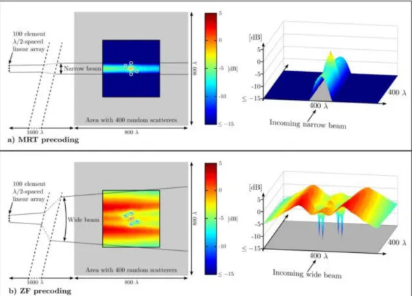
8Figure 2.5.1 Linear precoding within a scattering environment of size 800 ×800 [3]. ... 24

9Figure 2.5.2 Spectral efficiency Vs Energy efficiency [4] ... 25

10Figure 2.5.3 International Jamming [17] ... 26

11Figure 2.6.1 Per-cell rate vs. antenna number, 2-cell network, Gaussian distributed AτAs with = 10 degrees [22] ... 28

12Figure 2.6.2 BER vs. number of receive antennas [21] ... 29

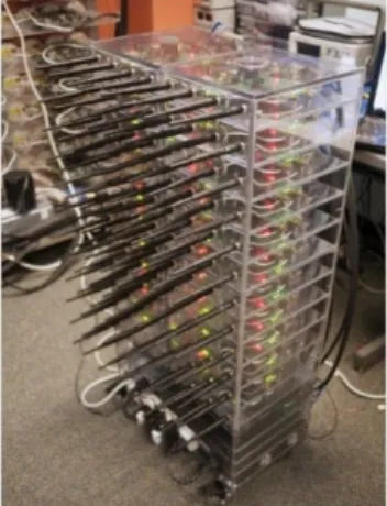
13Figure 2.6.3 The prototype of Argos with 16 modules and 64 antennas. Left: front side. Right: back side [24] ... 29

14Figure 2.6.4 Two large antenna arrays at the base station side: on left: a cylindrical array with 128 patch antenna on right: a virtual linear array with 128 omnidirectional antenna positions [26]. ... 30

(10)

7 | P a g e

15Figure 2.6.5 The measurement area at the campus of the Faculty of Engineering (LTH). The two BS antenna arrays were placed on the same roof of the E-building during two measurement campaigns [26].

... 30

16Figure 2.6.6 Four users close to each other at MS 2, with LOS to the base station antenna arrays [26]. ... 31

17Figure 2.6.7 Average sum-capacity and sum-rates with linear precoding versus SNR with M = 10 antennas and K = 8 UTs [27]. ... 32

18Figure 3.0 Multi-cell Massive MIMO ... 34

19Figure 3.5.1 Spectral Efficiency Vs. Number of BS antennas showing the performance of ZF receiver with non-linear receivers [6] ... 37

20Figure 3.6.1 TDD scheme for Massive MIMO reciprocity protocol [6]. ... 38

21Figure 3.6.2 Massive MIMO system ... 38

22Figure 3.7.1 Block diagram showing multi-cell uplink scheme with linear detector ... 41

24Figure 3.8.1 Outage probabilities of conventional ZF and MMSE vs. V-BLAST [14] ... 42

25Figure 3.10.2 Precoding scheme in multi-cell massive MIMO ... 44

26Figure 4.2.1 Specific coordinated beamforming [20] ... 50

27Figure 4.2.2 MIMO cooperation [21]. ... 50

28Figure 4.2.3 Single and multiple relay case [24] ... 52

29Figure 4.3.1 Iterative Receiver [26] ... 53

30Figure 4.3.2 Channel Characteristic Curve [26] ... 55

31Figure 4.4.1 Uplink Pilot Contamination ... 56

32Figure 4.4.2 Conventional TDD Frame ... 58

33Figure 4.4.3 MR Detection SE Vs number of UTs ... 63

34Figure 4.4.4 ZF Detection SE Vs number of UTs... 64

35Figure 4.4.5 Average Spectral Efficiency and number of UTs Vs increase number of BS antennas M with f=3, SNR=0db ... 64

36Figure 4.5.1 Point-to-Point case reciprocal model [65] ... 66

37Figure 5.3.1. TDD protocol format ... 76

38Figure.5.3.2 Block diagram shows different UTs and BS reciprocity operations ... 77

Fig. 39. Block diagram shows different UTs and BS reciprocity operations ... 77

40Figure 5.4.1 (b) Map connection overview ... 78

41Figure 5.4.1(a) CSI map ... 78

42Figure 5.4.2 Conception of CSI Map representing an indoor scenario ... 78

43Figure 5.5.1 Flowchart of CSI Learning Algorithm ... 79

44Figure. 5.8.2. Spectral Efficiency Vs. Number of antennas ... 82

45Figure 5.8.1. Sum-rate Vs Number of antennas ... 81

46Figure. 5.8.3. Energy Efficiency Vs. Number of antennas ... 82

47Figure 5.8.4. Hit ratio with respect to the number of TDD sessions ... 83

48Figure 6.3.1: Time-Shifted frames of Class 3 UTs ... 89

49Figure 6.4.1 User classification algorithm ... 89

50Figure 6.5.1 Greedy Pilot Allocation Algorithm ... 90

51Figure 6.6.1 Spectral Efficiency Vs M ... 91

52Figure 6.6.2 Energy Efficiency Vs M ... 92

53Figure 6.6.3 EE Vs Class index ... 92

54Figure 6.6.4 Classes indices from 1 to 30 Vs EE ... 93

55Figure 6.6.5 User Distribution among 21 Classes... 93

56Figure 6.6.6 User Distribution among 60 Classes... 94

57Figure 7.2.1 Fading effect ... 97

58Figure 7.2.2 Shadowing regions indoor ... 97

59Figure 7.2.3 Shadowing region outdoor ... 97

(11)

8 | P a g e

List of Tables

1Table 4.2.1 Interference mitigation techniques [17] ... 49

2Table 4.2.2 A cooperative MIMO channel model based on the WINNER II channel model [21]. ... 51

3Table 4.4.1 Estimation Methods and performance Analysis ... 57

4Table 5.8.1 Parameters ... 81

Nomenclature

General Symbols

(.)T denote transpose

(.)H Hermitian transpose

(.)* denote the conjugate

det(A) denote the determinant of A

⊙ denote element-wise multiplication

‖ ‖ denote the Frobenius norm and used for L2_-norm.

max {.}

maximum value of a set

min {.}

minimum value of a set

E [.]

statistical expectation

Ɲ , � complex circular symmetric normal distribution

H

channel coefficient matrix

K Number of users per cell

M Number of antennas per base station

L Number of cells

� Pilot sequence length

S Symbol vector

y signal vector

Standard deviation

P Power vector

[.]UL _{Corresponds to Uplink session}

Note:

Bold small letter, used to denote vectors Bold capital letter, used to denote matrix

General Abbreviations

BS Base Station

UT User Terminal

LoS Line of Sight

DoF Degree of Freedom

SNR Signal to Noise Ratio

SINR Signal to Interference Noise Ratio

MIMO Multiple Input Multiple Output

MRC Maximal Ratio Combination

ZF Zero Forcing

MMSE Minimum Mean Square Error

DPC Dirty Paper Coding

TDD Time Division Duplexing

(12)

9 | P a g e

5G Fifth Generation

IoT Internet of the Things

CSI Channel State Information

QCSI Quantized Channel State Information

SDN Software Defined Network

NFV Network Function Virtualization

RRH Remote Radio Head

(13)

10 | P a g e

Chapter 1μ Introduction

This chapter will introduce a background on the 5th_{generation wireless technology demands and} features. Further, it will clarify the position and the scope of this research within the literature. After reading this chapter, the intention behind researching on 5th_{generation wireless networks and the scope} of this thesis will be clear.

1 T

HE

5

TH

G

ENERATION

W

IRELESS

C

OMMUNICATION

S

YSTEMS 1.1 The fifth Generation Demand Features

An enormous amount of data has to cross the network, and internet services deliver most of this data. The QoS demands, and the rapid growth in bandwidth make 4G mobile networks insufficient to afford user requirements. The next generation mobile network should provide a bandwidth from 100Mbps up to 1Gbps per User Terminal (UT), and a density of connection that exceeds 1M connection/Km2_and high-speed vehicles mobility of up to 500 km/hr and an End-to-End (E2E) delay less than 10ms [1]. The 5G network needs to be elastic to afford Network-as-a-Service (NaaS) and simple SDN control. Also, Power effective, Security and Cost-effective Services must be provided. Furthermore, Quality of Experience (QoE) and Network Intelligence (NI), should be included.

1.2 Ongoing Global Research and Framework on 5th Generation

Many projects on 5G are ongoing in both industry and academic. In this section, we will introduce the most important proposals. In Europe, the main leading projects are 5G Private Public Partnership (5G PPP) [2] and Horizon 2020[3]. China introduces the main project by IMT-2020 (5G) Promotion Group [4]. Intel Strategic Research Alliance (ISRA) [5] in the USA leads new research on 5G networks. In [6], a software defined decentralized mobile network architecture (SoftNet) suggests distributed data forwarding, a dynamically defined architecture, multi-RATs coordination, and decentralized mobility management. SoftNet afforded features, includes a flexible and high capacity network in contrast to 4G mobile networks.

C-RAN or Cloud Radio Access Networks provides low operating expenses, as well as high energy and spectral efficiency. It separates the baseband processing from the radio units, permitting the processing power to be shared at a central location. Thus, dropping the required element redundancy by splitting BBU and RRH, where BBU pool offered as a centralized cloud service and Remote Radio Heads (RRH’s) are distributed among the network ends. This architecture solves many challenges struggle network flexibility but introduce a new challenge by flooding front-haul links with signaling data to the Baseband Unit (BBU) resources [7]. Recent research on C-RAN virtualization reduces signaling overhead by logically grouping macro cells with collocated small cells that can provide the core network with a simplified overview [8]. C-RAN projects have been initiated in many organizations such as the European Commission’s Seventh Framework program and the Next Generation Mobile Networks (NGMN) project.

SoftRAN is a software-defined control plane applied to radio access networks. It integrates all base stations in a local area as a virtual big BS containing radio access elements and a central controller [9].

It's much easier to get a reception from someone if

there is an introduction versus randomly trying to get

in front of people~ Brad Feld

(14)

11 | P a g e

SoftRAN suggests a logically centralized entity, which makes control plane decisions for all the radio elements in the geographical area. Nevertheless, this architecture still lacks some elasticity, where user terminals deal with the virtual BS as a separate BSs. SoftRAN arranges this issue by running multiple handovers between the same pair of base stations.

2 M

OTIVATIONS AND

P

RIOR

W

ORK

In 2010, Thomas L. Marzetta from Bell Labs posted a paper [10] on what can be considered as a strive to make full use of MIMO. Let the number of base station antennas develop barring restriction in MU-MIMO scenarios. The first important phenomenon is that the effects of additive receive noise and small-scale fading disappear, as does intra-cellular interference among users. The only remaining impairment is inter-cellular interference from transmissions that are associated with the equal pilot sequence used in channel estimation and that paper concludes that the throughput per cell and the number of users per cell are unbiased, the spectral efficiency is independent of the system bandwidth and required transmit strength per bit vanishes. Although some marvelous consequences are a situation to the system model and propagation assumptions used in the paper, Dr. Marzetta pointed out an essential route in which mobile systems may evolve. Scaling up MIMO provides many extra degrees of freedom in the spatial domain than any of trendy systems. This issue rescues us from the state of affairs that wireless spectrum has to turn out to be congested and expensive, mainly in frequency bands beneath 6 GHz. In contrast to traditional MU-MIMO with up to eight antennas, we name MIMO with a large variety of antennas “massive MIMτ”, “very-large MIMτ” or “large-scale MIMO”.

In massive MIMO operation, we take on consideration an MU-MIMO scenario, where a base station geared up with a large number of antennas serves many terminals in the same time-frequency resource. Processing efforts can be done at the base station side, and terminals have the simple and inexpensive hardware. Until now, many theoretical and experimental research has been executed in the massive MIMO context, e.g., [11]–[15]. These studies have proven that massive MIMO can considerably improve spectral efficiency while reducing radiated output power with the aid of at least an order of magnitude. In addition, real-time large MIMO testbeds are being carried out, and demonstrations are reported in [16], [17].

In light of this, massive MIMO can be considered a promising system for the next 5th generation wireless mobile technology. This is due to the high capacity, spectral and energy efficiency that can be afforded. For instance, in a scenario of 80 antennae at the BS and a sixteen UT Closely located with NLOS, a sum-rate capacity at the downlink reaches 40 b/s/Hz using Dirty Paper Coding (DPC) [18].

However,

certain essential characteristics of massive can limit the performance and challenge the

implementation of this technology. That is to say, uplink pilot contamination, limited pool of

orthogonal pilot sequence within the coherence interval and training overhead are considered

as the main aspects that face the implementation of massive MIMO.

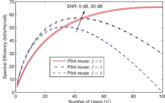
The use of TDD scheme in massive MIMO is considered as a higher alternative when channel reciprocity is regarded for channel estimation [19]. However, the principal constraint is the coherence interval length. The use of non-orthogonal pilot indicators in multi-cell introduces the trouble of pilot contamination. The effect of pilot contamination is shown to be profound in the multi-cell state of affairs with a high-frequency reuse factor of one. Some researchers suggest the use of fractional frequency reuse to mitigate the impact of pilot contamination [20]. However, several other researchers have proposed extraordinary techniques in reducing the outcomes of pilot contamination for a reuse factor heigher than one. The majority of the reviewed papers think about the worst-case situation and uniform distribution when analyzing the consequences of pilot contamination. Low bound on achievable rate have been derived based on best and imperfect channel estimation and for uniformly dispensed UTs in

L cells with a finite number of BS antennas [21]. Other viable causes of pilot contamination, such as

hardware impairment and non-reciprocal are also studied in [12], [22].

This work studies uplink pilot contamination in massive MIMO systems and proposes two novel techniques to mitigate pilot contamination by exploiting the coherence interval characteristics of UTs.

(15)

12 | P a g e

Also, the reduction in training overhead and transmitted energy makes this work a breakthrough in the literature.

3 C

ONTRIBUTIONS

The problem of pilot contamination has received significant interest from the ongoing research on massive MIMO. Theoretical evaluation has recognized pilot contamination as an imperative restriction on the throughput of massive MIMO systems [23]. Throughout this thesis, our goal is to propose techniques to mitigate uplink pilot contamination. Our contribution had proved its ability to mitigate contamination, increase sum-rate, increase energy and spectral efficiency as well as the number of user terminal per cell.

The contribution of this research can be presented as follows:

First, for the indoor scenario, we introduce the CSI Map, where BS stores the CSI of each UT at each position of the covered region. We use graph theory to represent this map. Each node stores a quantized version of the CSI, which is previously estimated from a UT in a particular location. The nodes are connected with directed weighted edges that represent the transition of a UT between two channel states. We develop an algorithm that creates and update the map during the learning phase, and we suggest the use of Expectimax search to predict the next possible CSI of a monitored UT within the map. Furthermore, we use Garbage Collector (GC) algorithm to remove rarely visited nodes to reduce the complexity of the CSI Map.

Second, another novel technique to reduce training overhead was introduced. In this contribution, we classify UTs based on their coherence interval into several classes. Users of the first class, i.e. high mobility users, were considered to upload their pilots in each frame similar to traditional reciprocity TDD protocol. In contrast, low mobility UTs related to class n must upload their pilots once every n frame due to their larger coherence interval. Exploiting the pilot sparsity of frames related to class n >1, we shift frames with pilots to an empty time space. The proposed method, reduce the number of uploaded pilots eventually as well as the training overhead. The added value of applying user classification with pilot shifting, reduce the uplink pilot contamination and increase the system performance in the dimension of energy and spectral efficiency. It also increases the system sum-rate and the cell density. Worth to mention that the proposed technique can be used jointly with any other pilot decontamination techniques if the number of UTs is still higher than the number of orthogonal pilots.

4 O

RGANIZATION

The organization of the thesis is as follows:

• Chapter 2 reviews the massive MIMO concept, including the advantages and challenges facing this technology.

• Chapter 3 was dedicated to massive MIMO channel measurements and processing. In this chapter, uplink and downlink processing will be considered including linear and non-linear processing.

• Chapter 4 introduce the interference challenge in 5G networks and focus on uplink pilot contamination in massive MIMO mobile technology. It also summarizes some literature techniques to mitigate uplink pilot contamination.

• Chapter 5 proposes our first novel technique to mitigate uplink pilot contamination in massive MIMO. It introduces the CSI map that will be used to predict channel rather than estimating it. The numerical results of applying this technique were also presented in this chapter.

• Chapter 6 proposes our second novel technique to mitigate uplink pilot contamination. In this chapter, we introduce the pilot shifting in sparse pilot frames. This method describes how to classify users based on their mobility profile and skip sending pilots for low mobility users. At the end of this chapter, numerical results were introduced to prove the ability of the proposed technique to overcome conventional massive MIMO.

(16)

13 | P a g e

5 C

ONFERENCES AND

P

UBLICATIONS

5.1

Refereed Papers

1- Title: Forecasting and Skipping To Reduce Transmission Energy In WSN Authors: Ahmad Abboud, Abdel-Karim Yazbek, Jean-Pierre Cances, Vahid Meghdadi Journal:International Journal of Research in Engineering and Science

Domain: Electronics Engineering Published: June 2016

ISSN: 2320-9364 Description:

The fundamental concept behind this research is the is the ability to use previously stored pattern at the base station to estimate the measured data from the sensor before requesting which limit the content of the transmitted to include only the error variance.

2- Title: Indoor Massive MIMO: Uplink Pilot Mitigation Using Channel State Information Map Authors: Ahmad Abboud, Jean-Pierre Cances, Ali H. Jaber, Vahid Meghdadi

Journal:_{Journal of Algorithms and Computational Technology} Domain: Networking and Internet Architecture

Year: 2016

Pre-Print: arXiv:1605.00082 Description:

This research proposes a novel method to mitigate uplink pilot contamination effect in an indoor Massive MIMO system by exploitation of stored channel state information CSI to precode new vectors based on the prediction.

[This work was introduced in “19th IEEE International Conference on Computational Science and Engineering (CSE 2016)- Paris, France”]

5.2 Submitted Papers

1- Title: Channel Coherence Classification with Pilot Shifting

Authors: Ahmad Abboud, Oussama Habachi, Jean-Pierre Cances, Vahid Meghdadi, Ali Jaber

Description:

In this work, we classify users based on their coherence interval length where channel training is done once each coherence interval for each group. Then we make use of the pilot sparsity in long coherence intervals to shift similar pilot sequences into an empty training slot.

[This work was accepted in 3nd International Symposium on Ubiquitous Networking (UNet'17) as Invited Paper].

2- Title: CSI Map for Indoor Massive MIMO

Description: An improved version of the Indoor massive MIMO paper that consider a garbage collection algorithm to decrease the size of the CSI map and upgrade the algorithm used to learn new CSI.

[This paper was accepted in “SAI Computing Conference 2017” and will be available in IEEE Explorer soon]

(17)

14 | P a g e

5.3 Papers in Preparation or Revision

1- Title: Spatio-temporal User Specific Mobility Profile in Smart Cities Wireless Networks Authors: Ahmad Abboud, Oussama Habachi, Jean-Pierre Cances, Vahid Meghdadi, Ali Jaber Description: This paper exploits the user mobility profile in wireless networks to improve decision making on various services in smart cities. As a methodology, Naïve Net is used to represent the conditional transition probability of specific user connected between sites in the network where the tessellation weight of the sites and the particular period of transition was taken as features. Then a decision network will represent the optimal utility to take action based on the transition probability of the Naïve net. The studied Model of User Mobility takes into consideration three dimensions (User specific, period specific and site specific) which make it flexible and powerful to query out critical what-if scenarios to make an optimal decision considering city resources management.

2- Title: Smart Massive MIMO: An Infrastructure Toward 5th Generation Smart Cities Network Authors: Ahmad Abboud, Jean-Pierre Cances, Vahid Meghdadi, Ali Jaber

Journal: arXiv preprint arXiv:1606.02107

Description: On the Optimizing of Wireless Networks and toward improving the future 5G Mobile Network Infrastructure, we propose a novel infrastructure that can serve for the next Smart City Network. Our proposed Infrastructure takes into consideration most future demands and challenges, includes Capacity, Reliability, Scalability, and Flexibility. To deal with these issues, we suggest a wireless network infrastructure that is based on latest technologies of Massive MIMO systems.

3-

Title: Concatenated Channel Estimation for Massive MIMO systems

Description:

This work introduces a novel idea that theoretically enables the

implementation of an unlimited number of user terminal within each cell without

encountering pilot contamination, even with a limited number of orthogonal pilot

sequences.

This technique is done by estimating the CSI in an initial frame and correct this CSI at

each training iteration using a short-reused pilot. The method considered useful only after

exploiting the coherence block overlapping. In other words, the correction phase is done

within the same coherence interval, which elongates the age of the CSI at each iteration.

6 R

EFERENCES

[1] “METIS 2020,” 2013. [τnline]. Availableμ httpsμ//www.metis2020.com/. [2] “5G-PPP,” 2016. [τnline]. Availableμ httpsμ//5g-ppp.eu/.

[3] “HτRIZτσ 2020,” 2016. [τnline]. Availableμ httpsμ//ec.europa.eu/programmes/horizon2020/. [4] “IMT-2020,” 2016. [τnline]. Availableμ httpμ//www.imt-2020.cn/en/.

[5] “Intel Labs,” 2013. [τnline]. Availableμ httpμ//blogs.intel.com/intellabs/2013/07/15/next-generation-wireless-communication-5g-transforming-the-wireless-user-experience/.

[6] H. Wang, S. Chen, H. Xu, M. Ai, and Y. Shi, “Softσetμ A software defined decentralized mobile network architecture toward 5G,” IEEE Netw., vol. 29, no. 2, pp. 16–22, 2015.

[7] M. Peng, C. Wang, V. Lau, and H. V. Poor, “Fronthaul-constrained cloud radio access networks: Insights and challenges,” IEEE Wirel. Commun., vol. 22, no. 2, pp. 152–160, 2015.

[8] A. W. Dawson, M. K. Marina, and F. J. Garcia, “τn the benefits of RAσ virtualisation in C-RAσ based mobile networks,” Proc. - 2014 3rd Eur. Work. Software-Defined Networks, EWSDN

2014, pp. 103–108, 2014.

[9] A. Gudipati, D. Perry, L. E. Li, and S. Katti, “SoftRAσμ Software defined radio access network,” in Proceedings of the second ACM SIGCOMM workshop on Hot topics in software defined

networking, 2013, pp. 25–30.

[10] T. L. Marzetta, “σoncooperative cellular wireless with unlimited numbers of base station antennas,” IEEE Trans. Wirel. Commun., vol. 9, no. 11, pp. 3590–3600, 2010.

(18)

15 | P a g e

Signal Process. Mag., vol. 30, no. 1, pp. 40–60, 2013.

[12] E. Björnson, J. Hoydis, and M. Kountouris, “Massive MIMτ Systems With σon-Ideal Hardware μ Energy Efficiency , Estimation , and Capacity Limits,” vol. 60, no. 11, pp. 7112– 7139, 2014.

[13] L. You, X. Gao, X.-G. Xia, σ. Ma, and Y. Peng, “Massive MIMτ Transmission with Pilot Reuse in Single Cell,” 2014 IEEE Int. Conf. Commun., no. JUNE 2014, pp. 4783–4788, 2014.

[14] E. Björnson, E. G. Larsson, and M. Debbah, “Massive MIMτ for Maximal Spectral Efficiencyμ How Many Users and Pilots Should Be Allocated?,” in IEEE Transactions on Wireless

Communications, 2016, vol. 15, no. 2, pp. 1293–1308.

[15] H. Q. σgo, E. G. Larsson, and T. L. Marzetta, “Energy and spectral efficiency of very large multiuser MIMτ systems,” IEEE Trans. Commun., vol. 61, no. 4, pp. 1436–1449, 2013. [16] A. Osseiran et al., “Scenarios for 5G mobile and wireless communicationsμ The vision of the

METIS project,” IEEE Commun. Mag., vol. 52, no. 5, pp. 26–35, 2014.

[17] J. Vieira et al., “A flexible 100-antenna testbed for Massive MIMτ,” in 2014 IEEE Globecom

Workshops, GC Wkshps 2014, 2014, pp. 287–293.

[18] X. Gao, τ. Edfors, F. Rusek, and F. Tufvesson, “Massive MIMτ performance evaluation based on measured propagation data,” pp. 1–12, 2015.

[19] T. L. Marzetta, “Massive MIMτμ An Introduction,” Bell Labs Tech. J., vol. 20, pp. 11–22, 2015. [20] L. Su and C. Yang, “Fractional frequency reuse aided pilot decontamination for massive MIMτ

systems,” in IEEE Vehicular Technology Conference, 2015, vol. 2015.

[21] M. M. System, O. Elijah, S. Member, C. Y. Leow, and T. A. Rahman, “A Comprehensive Survey of Pilot Contamination in Massive MIMO—5G System,” IEEE Commun. Surv. Tutorials, vol. 18, no. c, pp. 905–923, 2015.

[22] E. Björnson, J. Hoydis, M. Kountouris, and M. Debbah, “Hardware impairments in large-scale MISO systemsμ Energy efficiency, estimation, and capacity limits,” in 2013 18th International

Conference on Digital Signal Processing, DSP 2013, 2013.

[23] J. Jose, A. Ashikhmin, T. L. Marzetta, and S. Vishwanath, “Pilot contamination and precoding in multi-cell TDD systems,” IEEE Trans. Wirel. Commun., vol. 10, no. 8, pp. 2640–2651, 2011.

(19)

16 | P a g e

Chapter 2μ Massive MIMτ τverview

This chapter introduces the intention behind increasing the number of antennas at the base station as well as the evolution from MIMO to Massive MIMO. In details, it investigates the Massive MIMO system, its benefits, and its challenges. Furthermore, we investigate the uplink pilot contamination problem and the used method in the literature to mitigate uplink pilot contamination will be discussed.

1 F

ROM

MIMO

TO

M

ASSIVE

MIMO

Generally, MIMO systems are divided into two categories: single-user MIMO (SU-MIMO) and multi-user MIMO (MU-MIMO). In SU-MIMO, the transmitter and receiver are outfitted with more than one antennas. The performance is enhanced in terms of coverage, link reliability, and sum rate can be executed via strategies such as beamforming, diversity-oriented space-time coding, and spatial multiplexing of numerous data streams. These methods cannot be thoroughly used at the same time, therefore we commonly add a tradeoff between them. For example, adaptive switching between spatial diversity and multiplexing schemes is adopted in LTE [1].

The situation with MU-MIMO is radically different. The wireless channel is now spatially shared by way of different UTs, and the users transmit and obtain barring joint encoding and detection amongst them. By exploiting differences in spatial signatures at the BS antenna array caused by way of spatially dispersed users, the BS communicates concurrently to the users. Thus, overall performance beneficial properties regarding sum rates of all users can be impressive. An important venture is, however, the interference among the co-channel users [2]. Signal processing in MU-MIMO regularly targets at suppressing inter-user interference, thus spatial channel knowledge turns into another indispensable in contrast to SU-MIMO.

Massive MIMO is a new notion that makes use of hundreds of antennas at the BS to serve tens of UTs simultaneously in the same time-frequency resource. Massive MIMO mostly approves us to reap all the benefits of conventional MIMO on a large scale. In Massive MIMO systems, a huge number of BS antennas enhance spectral efficiency and radiated energy efficiency as compared to the present wireless technologies. The BS antennas make use of the idea of beamforming using transmitting solely in the preferred directions so that the radiated energy is centered in a small area and interference is minimized [3].

Massive MIMO systems enable an extend in theoretical sum-rate and a reduction in uplink (UL) and downlink (DL) energy consumption. The uplink power should be scaled down by way of relatively increasing the number of BS antennas [4]. All these motivations make Massive MIMO a conceivable solution for future broadband technologies. As the range of antennas at the BS increases, linear receivers such as (MRC) and (MMSE) turn out to be optimal. As a result, the acquisition of CSI turns into fundamental for the operation of Massive MIMO systems [5], [6]. Note that the acquisition of CSI is achieved via pilot sequences. Since the pilots require orthogonality between the antennas and all users operate in the same time-frequency resource, such structures have an inherent quandary due to pilot contamination. It is shown that the principal limiting element in growing the number of BS antennas is the pilot contamination [6].

Life is like riding a bicycle. To keep your balance,

(20)

17 | P a g e

2 M

ASSIVE

MIMO

S

YSTEM 2.1 System Characteristics

Massive MIMO is a form of MU-MIMO structures where the variety of BS antennas and the numbers of UTs are huge. In Massive MIMO, thousands of BS antennas concurrently serve tens or hundreds of users in the same frequency resources. Some essential points of Massive MIMO are:

2.1.1 Scalability

The BS learns the channels via uplink training, with TDD operation. The time required for channel estimation is impartial of the number of BS antennas. Therefore, the broad range of BS antennas can be made as large as favored with no extension in the channel estimation overhead. Furthermore, the signal processing at every UT is essential and does not depend on other UTs existence, de-multiplexing signal processing is carried out at the UTs. Adding or losing some UTs from service does no longer have an effect on other UT activities.

2.1.1.1 Massive MIMO prefers TDD Scheme

Using FDD, the channel estimation overhead relies upon on the number of BS antennas M. By contrast, using TDD, the channel estimation overhead is unbiased of M. In Massive MIMO, M is large, and hence, TDD operation is preferable. For instance, suppose that the coherence interval is

T = 200 symbols (corresponding to a coherence time of 1 ms and a coherence bandwidth of 200 kHz). Then, in FDD systems, the quantity of BS antennas and the amount of UTs are limited through M + K < 200, while in TDD systems, the constraint on M and K is 2K < 200. From fig 2.2.1, we can

see that the FDD place is tons smaller than the TDD region. With TDD, adding more antennas does now not affect the sources needed for the channel acquisition.

(21)

18 | P a g e

2 Figure 2.2.2 The Rice University Argos

Figure 2.2.1 indicates the overwhelming gain of TDD over FDD for UTs. The vertical axis is the number of BS antennas, and the horizontal axis is the quantity of UTs. The light-to-medium blue location indicates the gadget dimensions accessible with TDD versus the much smaller red area for FDD. The slot duration is four ms, which allows 35 km/h mobility at 1.9 GHz. To reduce pilot contamination, the orthogonal pilot sequences selected seven times longer than necessary.

2.1.2 Antenna Array Should Not be Physically Large

For instance, think about a cylindrical array of 128 antennas, comprising four circles of 16 dual-polarized antenna elements. According to [8], at 2.6 GHz, the distance between adjecent antennas is about 6 cm, which is 1/2 a wavelength, and hence, this array occupies a physical dimension of 28cm × 29cm solely.

2.1.3 Massive MIMO Offers Favorable Propagation

Favorable propagation, described as mutual orthogonality amongst the vector-valued channels to the terminals, is one of the key factors of the radio channel that is utilized in Massive MIMO [9]. However, there has been little work on this matter in detail. As the used number of BS antennas goes huge, Massive MIMO tends to have favorable propagation. This reality holds due to the regulation of large numbers.

2.2 Massive MIMO Processing

Processing in Massive MIMO takes place in TDD scheme within three phases, Channel Estimation (includes upload pilots), uplink data receiving and downlink data (see Fig 2.2.3).

(22)

19 | P a g e

The three stages are done within 2-time divisions that lag for not more than the coherence interval length.

2.2.1 Channel Estimation

At the reverse link, the BS needs the channel state information to become aware of the signals transmitted from the UTs in the uplink, and to precode the signals in the downlink. This channel information is acquired via the uplink training. Each user is assigned an orthogonal pilot sequence and sends his pilot sequence to the BS. Due to the pilot sequences orthogonality, the BS is aware of the pilots transmitted from all user terminals, and then estimates the channels based on the received pilot signals. Also, each user may need partial information of CSI to discover the signals transmitted from the BS coherently. Downlink training can typically obtain these statistics. Since the BS makes use of linear precoding strategies to beamform the indicators to the users, the user desires solely on the active channel reap to notice its favored signals. Hence, the BS can spend a brief time to beamform pilots in the downlink for channel acquisition at the UT.

2.2.2 Uplink Data

After channel estimation, the BS can receive the uploaded data for each UT using the estimated version of the CSI. This estimation is done at the same reverse link of the coherence interval. The uploaded data from each UT is assumed to share the same frequency-time domain, where the BS uses the spatial multiplexing signature acquired from the CSI to separate the received data streams. Linear receivers include (MRC, MMSE, ZF) can efficiently receive the uploaded data stream without the need for complex non-linear receivers.

2.2.3 Downlink Data

The third phase of the TDD frame is the downlink data phase. The forward link is typically considered shorter than the reverse link, where the downlink data only occupy it. Within the same coherence interval, the BS uses the estimated CSI to precode the downlink data stream. Many techniques can do precoding in Massive MIMO but due to the law of large number Massive MIMO systems can use linear precoders (as MRT, MMSE, and ZF) to perform the task.

3 M

ASSIVE

MIMO

T

YPES

3.1 Single-User MIMO

Owing to the physical hassle of terminals, the number of antennas at the terminal is typically a lot much less than M. Therefore, SU-MIMO structures fall into case 1 when a massive amount of antennas are geared up at the base station, and hence reap the advantages of channel orthogonalization if favorable channel propagation circumstance holds. However, the SU-MIMO channels can be extraordinarily correlated due to the fact of the short distance of antennas at the terminal side and viable line-of-sight

(23)

20 | P a g e

environment. From the energy efficiency point of view, the use of a massive antenna array to serve a single or a small quantity of UTs may additionally not be wise. Hence, in this case, the achieve of massive MIMO for SU-MIMO can also be limited.

4Figure 2.3.1 Single-User Massive MIMO

= √ + (2.3.1)

Denote by , the uplink SNR, by , the channel response vector, by , the symbole vector and by the AWGN noise vector.

3.2 Multi-User Massive MIMO

When more than one terminals are allowed to access identical time–frequency resource, MU-MIMO offers greater system efficiency in contrast to SU-MIMO. In this section, we take into consideration a single-cell MU-MIMO systems, where the BS is serving K UTs with every terminal being equipped with one antenna. The received signal at the BS of an uplink MU-MIMO system is:

= ∑ = √ + (2.3.2)

= √ + (2.3.3)

is M ×1 received signal matrix, . e.g. = [ … … ] represents the channel vector

between the BS antennas and the kth_UT, _{. e.g.} _{= [ … … ] represents the symbol} transmitted by kth UT and represents the Additive White Gaussian Noise (AWGN).

(24)

21 | P a g e

5Figure 2.3.2 Multi-user Massive MIMO System. M-antennas BS serves the K single antenna UT.

When K ≥ 2, the obtained signal of every UT interferes with those of the other terminals, and hence we should anticipate that the mutual information of every terminal for MU-MIMO is smaller than that for SU-MIMO given the same transmitted power at each terminal. However, when M K, the channel

orthogonalizing kicks in, such that the obtained signal of every terminal is nearly orthogonal, that is, interference-free in the favored sign house below favourable channel propagation condition. Also, given that the terminals are autonomous, the favorable channel propagation condition is usually comfortable due to the fact the antennas at the terminals are almost uncorrelated and uncoupled [8]. It suggests that the Massive MIMO is the desire of the MU-MIMO setup.

3.3 Multi-User Massive MIMO with Multi-Cell scenario

In this section, we contemplate the restriction of non-cooperative cellular multiuser MIMO systems as

M grows without limit. For a single cell, as properly as for multi-cell MIMO, the outcome impact of

letting M increase without limits is that thermal noise and small-scale Rayleigh fading vanishes. However, as we will discuss, with more than one cell the interference from distinct cells due to pilot contamination will persist. The idea of pilot pollution is novel in a cellular MU-MIMO context and is illustrated in Fig 2.3.3. However, used to be a problem in the context of CDMA, generally with the title “pilot contamination”. The channel estimate computed with the aid of the base station in cell l being contaminated from the pilot transmission of cell j. The BS in cell l will beamform its signal partially alongside the channel to the terminals in the adjacent cell. Due to the beamforming, the interference to cell j does not vanish asymptotically as M →∞. We reflect on consideration on a cellular multi user MIMO-OFDM system with hexagonal cells and NFFT subcarriers. All cells serve K independent terminals and have M antennas at the BS. The BSs are assumed non-cooperative. The M × K composite channel matrix between the K UTs in cell l and the BS in cell j is denoted by . Relying on reciprocity, the down link channel matrix between the BS in cell j and the terminals in cell l is presented by . The received signal at the j-th BS will be as follows:

= ∑= ∑ = √ + (2.3.4)

(25)

22 | P a g e

6Figure 2.3.3 The base station in l-th cell and the k-th user in j-th cell

3.4 Distributed Massive MIMO

Distributed Massive MIMO can be handled as a distinct case of MU-MIMO to additionally supply greater system capacity using dispersed deployed antennas to transmit and receive signals. One scheme of disbursed Massive MIMO is to allow cooperation between the BS’s in distinctive cells which reduces the inter-cell interference. However, synchronization turns into a quintessential problem even for dispensed antennas at the same BS. In some cases, the massive quantity of antennas at the base station can additionally be positioned in unique places [11] (e.g., on tops of buildings). In this case, synchronization is one issue, and the inexpensive RF front end might also introduce greater problems.

4 O

N THE

M

ASSIVE

MIMO

E

FFECT

This section will discuss the effect of increasing the dimension of antennas on the overall system performance. To focus on the effect of increasing the number of antennas at the BS and within the UTs we will consider a single cell Massive MIMO scenario where K UTs with one antenna each, served with one BS holding M antennas. Two scenarios can be discussed, first considering increasing

M without bounds where M >>K, the second scenario consider both M and K increased without

bounds where ≈ .

One of the most interesting performance metric to be considered in any communication system is the transmitted mutual information which is the measure of bit per channel use. Using the model in (2.3.3) and considering a Gaussian distribution of the symbols, the instantaneous mutual information, which is also referred as system capacity [12], is expressed as follows:

= ��g de� +

= ��g de� + (2.4.1)

Since H is a random matrix [13], we can calculate the ergodic capacity �{ } as follows:

�{ } = M �{��g + � } (2.4.2)

where � denotes the eigenvalues of the normalized Wishart matrix � [14].

Considering the first scenario M >> K, where is Gaussian i.i.d. random matrix, by the law of large numbers, � = � tends to . This result means that, when M tends to ∞, the eigenvalues in (2.4.2) tends to . For M >> K, the expectation of mutual information can be written as:

(26)

23 | P a g e

Considering the second scenario, where M and K both increase without bounds, with a ratio, Ϝ = , the eigenvalues will converge statistically according to Marchenko-Pastur law which is given in the following theorem:

Theorem 2.3.1: Consider a matrix ℂ × with i.i.d. entries

√ , , such that , has zero

mean and unit variance. As , → ∞ with → , ∞ , the eigenvalues distribution =

converges weakly and almost surely to a nonrandom distribution function with a density function that can be presented as follow:

= − − + ₊ _{√ −} + ₋ +

where = − √ , = + √ and = _{{ }} represents the Dirac function.

The proof of Theorem 2.3.1 can be found in [15].

Referring to the graphical illustration of the eigenvalues distribution in the figure below, one can infer the deterministic state of the eigenvalues as the number of BS antennas relative to the number of users, increases without limits (here referred as c).

5 M

ASSIVE

MIMO

B

ENEFITS

Massive MIMO technology exploits phase-coherent, where computationally it is a simple processing of signals from all the antennas at the base station. Some unique advantages of a large MU-MIMO system are mentioned below.

5.1 Increasing Capacity

The increase in capacity results from the aggressive spatial multiplexing used in massive MIMO. The quintessential precept that makes the dramatic increase in energy efficiency viable is that with a large number of antennas, power can be centered with intense sharpness into small areas in space.

The underlying physics is the coherent superposition of wavefronts. By accurately shaping the signals sent out through the antennas, the BS can make sure that all wavefronts jointly emitted using all antennas add up constructively at the places of the dedicated terminals, and destructively almost everywhere else. Interference between terminals can be suppressed even similarly with the aid of linear precoder, e.g., MMSE, ZF. However, this may come at the cost of more transmitted power.

(27)

24 | P a g e

By numerical analysis, the essential exchange between the energy efficiency regarding the total number of transmitted bits per Joule per terminal receiving provider of energy spent, and spectral efficiency relating to a total number of transmitted bits per Hz. The figure below (Figure 2.5.2) illustrates the relationship for the uplink, from the terminals to the base station.

Figure 2.5.2, indicates the exchange off for two cases: in purple, a reference system with one single antenna serving a single UT. In green, a system with one hundred antennas serving a single UT using traditional beamforming and at last, a massive MIMO system with a hundred antennas simultaneously serving forty UT's (blue, using ZF and red, using MRC).

Using of MRC receivers in contrast with ZF is not only its simpler complexity by using multiplication of the obtained signals by the conjugate channel responses, but also that it can be carried out in a distributed fashion, independently of every antenna unit. While ZF additionally works well for a traditional or moderate dimension MIMO system, MRC typically does not. The key factor behid the performance of MRC in massive MIMO is that the channel responses associated with distinct terminals tend to be nearly orthogonal when the number of base station antennas is large. The prediction in (Figure 2.5.2) relies primarily on an information theoretical analysis that considers intra-cell interference, as well as the energy cost and bandwidth of using pilots to estimate CSI in a high-mobility scenarios.

(28)

25 | P a g e

9Figure 2.5.2 Spectral efficiency Vs Energy efficiency [4]

The purpose that the average spectral efficiency ten times higher than in traditional MIMO is that many terminals are served simultaneously, in the same time-frequency resource. When running in the 1 bit/dimension/UT regime, there is additionally some evidence that inter-symbol interference can be handled as extra thermal noise, therefore offering a way of disposing OFDM as an ability to combat inter-symbol interference [16].

To recognize the scale of the potential beneficial properties of Massive MIMO, think about an array consisting of 6400 omnidirectional antennas. A whole structure aspect of 6400 × ( ) ≈ 40 m2, transmitting with a complete power of 120 Watts (every antenna radiating about 20 mW) over a 20 MHz bandwidth in the band (1900 MHz). The array serves 1000 fixed terminals randomly allocated in a disk of radius 6 km centered on the array, every terminal having an 8dB gain antenna. The peak of the antenna array is 30m, and the height of the terminals is 5m. Using the Hata-COST231 model we locate that the route loss is 127 dB at 1 km distance and the range-decay exponent is 3.52. With log-normal shadow fading with 8 dB standard deviation and 9 dB noise at the receiver, one-quarter of the TDD frame is spent on the transmission of uplink pilots. Furthermore, it is assumed that the channel is significantly steady over periods of 164 ms to estimate the channel gains with enough accuracy. The downlink data is transmitted through MRT beamforming mixed with strength control, where the 5% of the users that have the worst channels are omitted from service. Numerical averaging over random terminal places over the shadow fading indicates that 95% of the terminals will obtain a throughput of 21.2 Mb/s/UT. According to [3], the array in this example will provide the 1000 terminals a full downlink throughput of 20 Gb/s, ensuring in a sum spectral efficiency of 1000 bits/s/Hz. This given, would be sufficient to grant 20 Mbit/s broadband service to each of a 1000 UTs. The max-min power control provides similar service concurrently to 950 terminals. Other types of power control associated with time-division multiplexing ought to accommodate various traffic needs of a larger set of terminals. The MRC receiver and its counterpart MRT precoding are additionally regarded as matched filtering (MF) in the literature.

(29)

26 | P a g e

5.2 Increase Robustness Against Man-Made Interference and International Jamming

A serious cyber- security risk is the intentional jamming of private wireless systems (see Fig 2.5.3), that seems to be little regard to the public. Simple jammers can be sold off the Internet for a few $100, and tools that used to be military-grade can be put collectively using off-the-shelf software radio-based platforms for a few $1000. Numerous latest incidents, specifically in public security applications, illustrate the magnitude of the problem. During the EU summit in Gothenburg, Sweden, in 2001, demonstrators used a jammer positioned in a close by the apartment and while major phases of the riots, the chief commander could not attain any of the engaged seven-hundred police officers [17].Due to the shortage of bandwidth, spreading data over frequency is no longer possible, so the only way of enhancing the performance of wireless communications is to use a couple of antennas. Massive MIMO provides many extra DoF that can be used to cancel signals from intentional jammers. If Massive MIMO is implemented through the usage of uplink pilots for channel estimation, then smart jammers should make hazardous interference with modest transmission power. However, further smart implementations by joint channel estimation and decoding need to be capable to considerably lower that problem.

10Figure 2.5.3 International Jamming [17]

5.3 Inexpensive and Low-Power Components

With Massive MIMO, expensive, ultra-linear 50W amplifiers used in traditional systems are changed by using 100's of cheap amplifiers with output power in the milli-Watt range. The distinction to traditional array designs, which use few antennas fed from high-power amplifiers, is significant. Several costly and cumbersome items, such as giant coaxial cables, can be eradicated. Massive MIMO reduces the constraints on accuracy and linearity of every item amplifier and RF chain. All that should be considered is their mixed action. In a way, Massive MIMO depends on the regulation of huge numbers to make sure that noise fading and hardware imperfections common out when signals from a huge number of antennas are mixed. The same characteristics that make Massive MIMO resilient in opposition to fading make the technology extraordinarily robust to failure. A Massive MIMO system has a huge spare of DoF. For example, with 200 antennas serving 20 terminals, 180 DoF are unused. This DoF can be used for hardware-friendly signal shaping. In particular, every antenna can transmit signals with minimum peak-to-average ratio [18] or even steady envelope [19] at a very modest penalty in phrase of the improved total radiated power. Such envelope signaling enables the use of extraordinarily low-cost and power-efficient RF amplifiers. The methods in [18], [19] should not be

(30)

27 | P a g e

burdened with traditional beamforming methods or equal-magnitude-weight beamforming techniques. This is with contrast with constant-envelope multi-user precoding where no beams are formed and the signals emitted through every antenna are no longer shaped using weighing of a symbol. Rather, a wave field is created such that when this wave field is sampled at the spots where the users are located, the terminals see precisely the signals that we favor them to see. The quintessential property of the Massive MIMO channel that makes this feasible is that the channel has a large null space: nearly anything can be put into this null space beside affecting what the terminals see. In particular, elements can be put into this null space that makes the transmitted waveforms fulfill the preferred envelope constraints. In spite of that, the advantageous channels between the base station and every terminal can take any signal group as input and does no longer require the use of PSK-type modulation. The extensively improved energy efficiency allows Massive MIMO systems to function with a total output RF power two orders of magnitude much less than with contemporary technology. This matter due to the fact the energy consumption of cellular base stations is a developing concern worldwide. Also, base stations that devour many orders of magnitude less power may want to be harvested by the wind or solar energy, and subsequently quickly deployed where no electricity.

5.4 Reduction in Latency

The furthermost restrictive factor in wireless communication systems is the presence of fading. The fading can render the obtained signal power very small at sometimes. This fact occurs when the signal dispatched from a base station travels through more than one path before it reaches the user terminal, and the waves ensuing from these multiple paths interfere destructively. Fading makes it difficult to construct low-latency wireless links. In case, the terminal is stuck in a fading dip, it must wait till the propagation channel has sufficiently modified until any symbol can be received. Massive MIMO depends on the regulation of large numbers and beamforming to keep away from fading problems so that fading no longer limits latency.

6 M

ASSIVE

MIMO

C

HALLENGES

6.1 Uplink Pilot Contamination

In an ideal way, every terminal in a Massive MIMO system is assigned an orthogonal uplink pilot sequence. However, the maximum range of orthogonal pilot sequences that can exist is upper bounded by the length of the coherence interval divided by the channel delay spread. In accordance to [20], for a typical working scenario, the maximum quantity of orthogonal pilot sequences in a one-millisecond coherence interval is estimated to be about 200. It is convenient to exhaust the reachable resources of orthogonal pilot sequences in a multi-cellular system. The impact of re-using pilots from one cell to another, and the related adverse consequences, is called “pilot contamination”. Specifically, when the service array correlates its acquired pilot signal with the pilot sequence related to a particular terminal, it indeed obtains a channel estimate that is contaminated by a linear mixture of channels to the different terminals that share the identical pilot sequence. Downlink beamforming primarily based on the contaminated channel estimate brings in interference that is directed to the terminals that share the identical pilot sequence. Similar interference is concord with uplink transmissions. This attentive interference grows with the number of antennas at an equal rate as the preferred signal [20]. Even in part, correlated pilot sequences leads to directed interference. Pilot contamination as a fundamental phenomenon is not particular to Massive MIMO. However, its impact on Massive MIMO seems to be an awful much extra profound than in traditional MIMO [5], [20]. According to [20], it used to be argued that pilot contamination constitutes a remaining limit on performance, when the number of antennas is elevated beside binding, at least with receivers that depend on pilot channel estimation. While this argument has been contested lately [21], at least beneath some particular assumptions on the power control used, it seems possible that pilot contamination needs to be dealt with in some way.

Atténuation des interférences dans les réseaux mobiles 5G : Contamination pilote des liaisons montantes dans le schéma massif MIMO TDD

HAL Id: tel-01619147

https://tel.archives-ouvertes.fr/tel-01619147

Atténuation des interférences dans les réseaux mobiles

5G : Contamination pilote des liaisons montantes dans le

schéma massif MIMO TDD

Ahmad Abboud

To cite this version:

Université de Limoges

École Doctorale Sciences et Ingénierie pour l’Information,

Mathématiques (ED 521)

Laboratoire XLIM, Département C

S

: Composants Circuits Signaux et Systèmes Hautes

Fréquences, ENSIL - Ecole Nationale Supérieure d'Ingénieurs de Limoges

Thèse pour obtenir le grade de

Docteur de l’Université de Limoges

Spécialité : Gestion des interférences dans le réseau mobile 5G

Présentée et soutenue par

Ahmad Abboud

Le 22 septembre 2017

Thèse dirigée par Jean-Pierre Cances, Ali Jaber et Vahid Meghdadi

JURY :

Président du jury

M. Gilles Burel, Professeur des Universités, UBO (Université de Bretagne

Occidentale), Université de Bretagne Occidentale, laboratoire Labsticc

Rapporteurs

M. Guillaume Ferré: MCF HDR, Laboratoire IMS Bordeaux, ENSEIRB Mat-Méca

M. Samir Saoudi, Professeur des Universités, Institut Mines-Télécom Atlantique

Examinateurs

M. Yannis Pousset, Faculté de Sciences Fondamentales et Appliquées, Université

de Poitiers, labo Xlim, axe SRI

M. Vahid Meghdadi, directeur, Co-encadrant de thèse, ENSIL Limoges, 16 rue

Atlantis, 87068 Limoges cédex, Labo: Xlim, axe SRI

M. Jean-Pierre Cances, directeur, Co-encadrant de thèse ENSIL Limoges, 16 rue

Atlantis, 87068 Limoges cédex, Labo: Xlim, axe SRI

Interference Mitigation in 5G Mobile Networks

Abstract

Acknowledgment

First, I would like to express my elite gratefulness and appreciations to my first supervisor

Prof. Jean-Pierre Cances for his supervision and provision. I would like to thank him for

inspiring my research, for tolerating me to grow as a researcher, and for providing

me this valuable prospect to follow a Ph.D. I am also thankful for my second,

supervisors, Prof. Ali Jaber, from the Lebanese University, and I would like to thank Prof. Vahid

Megdadi, from the University of Limoges, for his insightful debates.

It is my great honor to work with, Dr. Oussam Habachi and I am thankful for his significant

contribution to this work.

Also, I would like to take this opportunity to thank my teachers from the high school, namely

Mr. Bassam Saad, Mr. Ali Elaik for their encouragements.

In the end, my superior gratitude goes to my family for their unconditional love and tremendous

support.

Thank you all for helping me in all my quests.

Ahmad Abboud

Table of Content

Contents

List of Figures

List of Tables

Nomenclature

General Symbols

max {.}

maximum value of a set

min {.}

minimum value of a set

E [.]

statistical expectation

H

channel coefficient matrix

General Abbreviations

Chapter 1μ Introduction

1 T

5

G

W

C

S

It's much easier to get a reception from someone if

there is an introduction versus randomly trying to get

in front of people~ Brad Feld

2 M

P