Creative Destruction and Subjective Well-Being

HAL Id: halshs-01496948

https://halshs.archives-ouvertes.fr/halshs-01496948

Submitted on 28 Mar 2017

HAL is a multi-disciplinary open access archive for the deposit and dissemination of sci-entific research documents, whether they are pub-lished or not. The documents may come from teaching and research institutions in France or abroad, or from public or private research centers.

L’archive ouverte pluridisciplinaire HAL, est destinée au dépôt et à la diffusion de documents scientifiques de niveau recherche, publiés ou non, émanant des établissements d’enseignement et de recherche français ou étrangers, des laboratoires publics ou privés.

Philippe Aghion, Ufuk Akcigit, Angus Deaton, Alexandra Roulet

To cite this version:

Philippe Aghion, Ufuk Akcigit, Angus Deaton, Alexandra Roulet. Creative Destruction and Subjec-tive Well-Being. American Economic Review, 2016, 106 (12), pp.3869-3897. �10.1257/aer.20150338�. �halshs-01496948�

3869

Creative Destruction and Subjective Well-Being

By Philippe Aghion, Ufuk Akcigit, Angus Deaton, and Alexandra Roulet*

In this paper we analyze the relationship between turnover-driven growth and subjective well-being. Our model of innovation-led growth and unemployment predicts that: _{(i) the effect of creative} destruction on expected individual welfare should be unambiguously positive if we control for unemployment, less so if we do not; _{(ii) job}

creation has a positive and job destruction has a negative impact on well-being; _{(iii) job destruction has a less negative impact in} areas with more generous unemployment insurance policies; and

(iv) job creation has a more positive effect on individuals that are

more forward-looking. The empirical analysis using cross-sectional MSA _{(metropolitan statistical area)-level and individual-level data} provide empirical support to these predictions. _{(JEL I31, J63, J65,}

O33, O38₎

Does higher _{(per capita) GDP or GDP growth increase happiness? The existing} empirical literature on happiness and income looks at how various measures of sub-jective well-being _{(SWB) relate to income or income growth, but without looking} in further detail at what drives the growth process and at how the determinants of growth affect well-being. In this paper, we provide a first attempt at filling this gap.

More specifically, we look at how an important engine of growth, namely Schumpeterian creative destruction with its resulting flow of entry and exit of firms and jobs, affects SWB differently for different types of individuals and in different types of labor markets.

* Aghion: College de France, 3 rue d'Ulm, 75006, Paris, France, London School of Economics, NBER, and CIFAR (e-mail: paghion@fas.harvard.edu); Akcigit: University of Chicago, 1126 E. 59th Street, Chicago, IL 60637, and NBER (e-mail: uakcigit@uchicago.edu); Deaton: Princeton University, 361 Wallace Hall, Princeton, NJ 08544, and NBER (e-mail: deaton@princeton.edu); Roulet: Harvard University, Littauer Center, 1805 Cambridge Street, Cambridge, MA 02138 (e-mail: aroulet@fas.harvard.edu). The authors are grateful to the Gallup organization for permitting the use of the Gallup Healthways Well-Being Index data. For very help-ful comments and discussions, we thank Harun Alp, Marios Angeletos, Roland Benabou, Anne Case, Henry Farber, Fabrice Murtin, Jeremy Pearce, Richard Rogerson, Stefanie Stantcheva, Francesco Trebbi, Fabrizio Zilibotti, seminar or conference participants at Princeton, CIFAR, Columbia, Zurich, Harvard, the London School of Economics, the NBER Summer Institute-Income Distribution and Macroeconomics group, the Firm and Technology Dynamics conference at the University of Nottingham, the ASSA meetings in Boston, and the IEA Annual Congress in Amman, and the referees of this journal. Deaton acknowledges funding support from the Gallup organization, with whom he is a consulting senior scientist, and from the National Institute of Aging through the NBER, grants 5R01AG040629–02 and P01 AG05842–14, and through Princeton’s Roybal Center for Translational Research on Aging, Grant P30 AG024928. Akcigit gratefully acknowledges financial support from the National Science Foundation, Ewing M. Kauffman Foundation, and from the Alfred P. Sloan Foundation. Roulet gratefully acknowledges financial support from the NSF-IGERT Program in Inequality and Social Policy at Harvard University and the NBER Pre-doctoral Fellowship.

† _{Go to http://dx.doi.org/10.1257/aer.20150338 to visit the article page for additional materials and author} disclosure statement(s).

Thus, in the first part of the paper we develop a simple Schumpeterian model of growth and unemployment to organize our thoughts and generate predictions on the potential effects of turnover on life satisfaction. In this model, growth results from quality-improving innovations. Each time a new innovator enters a sector, the worker currently employed in that sector loses her job and the firm posts a new vacancy. Production in the sector resumes with the new technology only when the firm has found a new suitable worker. Life satisfaction is captured by the expected discounted valuation of an individual’s future earnings. In the model, a higher rate of turnover has both direct and indirect effects on life satisfaction. The direct effects are that, everything else equal, more turnover translates into both a higher probabil-ity of becoming unemployed for the employed, which reduces life satisfaction, and a higher probability for the unemployed to find a new job, which increases life sat-isfaction. The indirect effect is that a higher rate of turnover implies a higher growth externality and therefore a higher net present value of future earnings: this enhances life satisfaction. Overall, a first prediction of the model is that a higher turnover rate increases well-being more when controlling for aggregate unemployment than when not controlling for aggregate unemployment. A second prediction is that job creation increases and job destruction decreases well-being. A third prediction is that job destruction has a less negative effect on well-being, the more generous are unemployment benefits. A fourth prediction is that job creation increases future well-being more for more forward-looking individuals.1

In the second part of the paper we test the predictions of the model using cross-sectional metropolitan statistical area _{(MSA)-level US data. To measure} cre-ative destruction we follow Davis, Haltiwanger, and Schuh (1996) and use their mea-sure of job turnover, defined as the job creation rate plus the job destruction rate.2

The data come from the Census Bureau's Business Dynamics Statistics (BDS) and are at the MSA level. In addition, we also use the Longitudinal Employer-Household Dynamics (LEHD) data from the Census Bureau, which provide information on hires, separations, employment, and thus turnover, also at the MSA level. To mea-sure SWB, we use the Cantril ladder of life from the Gallup Healthways Well-Being Index _{(Gallup), which asks individuals about both current and future well-being. The} Cantril ladder is based on the following questions: “Imagine a ladder with steps num-bered from 0 at the bottom to 10 at the top; the top of the ladder represents the best possible life for you and the bottom of the ladder represents the worst possible life for you. On which step of the ladder would you say you personally feel you stand at this time? And which level of the ladder do you anticipate to achieve in five years?”3

We investigate whether Schumpeterian creative destruction affects these mea-sures of well-being positively or negatively, by regressing our meamea-sures of SWB on our creative destruction variables. The empirical analysis using cross-sectional MSA-level data on SWB and job turnover vindicates the theoretical predictions: 1 _{In the online Appendix, we characterize the transitional dynamics of the model and also extend the analysis} to the case where job destruction can be partly exogenous, or to the case where the turnover rate is endogenously determined by a free entry condition.

2 _{We have also looked at firm turnover, namely the sum of the establishment entry rate and the establishment} exit rate, with similar results.

3 _{In online Appendix A2, we also check the robustness of our results to a SWB measure from another dataset:} the Life Satisfaction question from the Behavioral Risk Factor and Surveillance System, which asks respondents “In general how satisfied are you with your life?”

namely, we find that: _{(i) the effect of creative destruction on well-being is positive} when we control for MSA-level unemployment and less so if we do not; (ii) the effects of job creation and job destruction on well-being are positive and negative, respectively; and (iii) job destruction has less negative effect when unemployment benefits are higher. Moreover, we find some evidence that job creation has a more positive impact on future well-being for more forward-looking individuals when we use income, age, and education to proxy for patience. These results are not only con-sistent with the theory, but they are also remarkably robust. In particular they hold whether looking at well-being at MSA level or at individual level, or whether using the BDS or the LEHD data to construct our proxy for creative destruction.

The paper relates to two main strands of literature. First, to the literature on inno-vation-led growth, job turnover, and unemployment (e.g., see Davis, Haltiwanger, and Schuh 1996; Mortensen and Pissarides 1998; Aghion and Howitt 1994, 1998; and Aghion, Akcigit, and Howitt 2014). In particular Aghion and Howitt (1994, 1998_{) and Mortensen and Pissarides (1998) develop Schumpeterian models of} growth through creative destruction, where growth is driven by quality-improving innovations by new entrants that make existing firms and jobs become obsolete. In any sector where new entry occurs, the incumbent firm closes down, therefore the worker employed by the incumbent firm loses her job whereas the entering firm in the sector posts a new vacancy. Equilibrium unemployment results from assuming labor market frictions in the form of a Poisson matching rate between new vacan-cies and workers looking for a new job. These papers point to two opposite effects of growth on unemployment. One is a “capitalization” effect whereby more growth reduces the rate at which firms discount the future returns from creating a new vacancy: this effect pushes toward creating more vacancies and thus toward reduc-ing the equilibrium unemployment. The counteractreduc-ing effect is a “creative destruc-tion” effect whereby more growth implies a higher rate of job destruction which in turn tends to increase the equilibrium level of unemployment. We contribute to this literature by looking at the counteracting effects of innovation-led growth on SWB.

Second, the paper contributes to the literature on SWB. In spite of a now large lit-erature on self-reported well-being,4 _{there is no general consensus on how seriously}

these SWB measures should be taken, or on exactly what they mean. Indeed some of the most exciting recent work _{(e.g., see Benjamin et al. 2012, 2014) is investigating} these fundamental questions.5 _{In this paper, we find that life satisfaction responds to} 4 _{In particular, in his seminal work, Easterlin (1974) provides evidence to the effect that, within a given} coun-try, happiness is positively correlated with income across individuals but this correlation no longer holds within a given country over time. This Easterlin paradox is often explained by the idea that, at least past a certain income threshold, additional income enters life satisfaction only in a relative way; Clark, Frijters, and Shields (2008) pro-vides a review of this large literature of which Luttmer (2005), Clark and Senik (2010), and Card et al. (2012) are prominent examples. Recent work has found little evidence of thresholds and a good deal of evidence linking higher incomes to higher life satisfaction, both across countries and over time. Thus in his cross-country analysis of the Gallup World Poll, Deaton (2008) finds a relationship between log of per capita GDP and life satisfaction which is positive and close to linear, i.e., with a similar slope for poor and rich countries, and, if anything, steeper for rich countries. Stevenson and Wolfers (2013) provide both cross-country and within-country evidence of a log-linear relationship between per capita GDP and well-being and they also fail to find a critical “satiation” income threshold. Yet these issues remain far from settled, see for example the reviews by Frey and Stutzer (2002), Layard (2011), or Graham (2009).

5 _{Benjamin et al. (2012) run three surveys to look at the extent to which, when facing two alternatives,} individ-uals choose the alternative from which they anticipate the highest SWB (as measured by the Cantril ladder). They find that SWB and choice coincide 83 percent of the time. Benjamin et al. (2014) survey students from US medical

the future growth prospects that are inherent in creative destruction, even in spite of the related short-run unemployment effects, and at the same time we provide some evidence of the validity and usefulness of self-reported well-being as a measure of expected future material well-being. Such findings have not been documented in the well-being literature so far and they provide further evidence of the usefulness of these well-being measures.

The paper is organized as follows. Section I develops the model and generates predictions on the effects of turnover on SWB, and how these effects depend upon individual or local labor market characteristics. Section II describes the data, the approach underlying the empirical analysis, and presents the empirical results. Section III considers several robustness checks. Section IV concludes the paper. The Appendix contains the proofs and the online Appendix presents extensions to the baseline framework, additional proofs, and extra tables.

I. Theoretical Analysis A. A Toy Model

In this section, we offer a simple model to motivate our empirical analysis. The source of economic growth is Schumpeterian creative destruction which at the same time generates endogenous obsolescence of firms and jobs. The workers in the obso-lete firms join the unemployment pool until they are matched to a new firm. Higher firm turnover has both a positive effect _{(by increasing economic growth and by} increasing employment prospects of unemployed workers) and a negative effect (by increasing the probability of currently employed workers losing their job) on well-being. Which effect dominates will in turn depend upon both individual char-acteristics _{(e.g., discount rate and risk-aversion) and characteristics of the labor} mar-ket (e.g., unemployment benefits). To keep the analysis tractable, in what follows we will consider a steady-state economy with exogenous entry, risk-neutral agents, and only endogenous job destruction. These assumptions will be relaxed in the online Appendix: Section A1.1 focuses on transitional dynamics, Section A1.2 considers a model with exogenous job destruction, Section A1.3 considers the implications of risk aversion, and Section A1.4 endogenizes entry in the theoretical model.

Production Technology and Innovation.—We consider a multi-sector Schumpeterian growth model in continuous time. The economy is populated by a set of infinitely-lived and risk-neutral individuals of measure one, and discount the future at rate ρ. Therefore the household Euler equation is simply

(1) r = ρ,

where r is the interest rate of the economy.

schools who enroll in the National Residence Matching Program; they find that individuals’ actual choice of resi-dence somewhat departs from individuals’ anticipated SWB rankings, and then they investigate possible sources of divergence between these SWB measures and revealed preferences. In the present paper, however, the predictions as to how creative destruction should affect individuals’ utility turn out to be fully mirrored by the empirical analysis using SWB measures and data.

The final good is produced using a continuum of intermediate inputs, according to the logarithmic production function

ln Y _t =

∫

j∈ ln y jt dj ,

where  ⊂

[

]

J _∈

[

]

Each intermediate firm produces using one unit of labor according to the follow-ing linear production function,

_{y jt = A jt l jt ,}

where _{l jt = 1 is the labor employed by the firm, and is the same in all sectors. Thus} the measure of inactive product lines is equal to the unemployment rate

u _t = 1 − J _t ,

where u denotes the equilibrium unemployment rate. Our focus will be on balanced growth path equilibrium, therefore, when possible, we will drop time subscripts to save notation.

Innovation and Growth.—An innovator in sector j at date t will move productivity in sector j from _{A jt−1 to}

_{A jt = λ A jt−1 ,}

where _{λ > 1. The innovator is a new entrant, and entry occurs in each sector with} Poisson arrival rate x which we assume to be exogenous . Upon entry in any sector, the previous incumbent firm becomes obsolete and its worker loses her job and the entering firm posts a new vacancy with an instantaneous cost cY .6 _{Production in that}

sector resumes with the new technology when the firm has found a new suitable worker.

Labor Market and Job Matching.—Following Pissarides (1990), we let (2) m( u _t , v _t ) = u _tα v _t1 −α

denote the arrival rate of new matches between firms and workers, where u _t denotes the number of unemployed at time t and _{v t denotes the number of vacancies. Thus} the flow probability for each unemployed worker to find a suitable firm is

m( u _t , v _t )/ u _t ,

6 _{In online Appendix A1.7, we provide sufficient conditions under which the incumbent firm in any sector will} choose to leave the market as soon as a new entrant shows up in that sector. The basic story is that, conditional upon a new entrant showing up, it becomes profitable for the incumbent firm to seek an alternative use of her assets.

whereas the probability for any new entrant firm to find a suitable new worker is

m( u _t , v _t )/ v _t .

In steady state, there will be a constant fraction of product lines that are vacant (of measure v _{), and the remaining fraction will be producing. We illustrate this} econ-omy in Figure 1.

Finally, we assume that in each intermediate sector where a worker is currently employed, the worker appropriates fraction β of profits whereas the complementary fraction _{(1 − β) accrues to the employer.}

Valuations and Life Satisfaction.—Life satisfaction is captured by the average present value of an individual employee, namely

W _t = u _t U _t + (1 − u _t ) E _t ,

where _{U t is the net present value of an individual who is currently unemployed,} and E _t is the net present value of an individual who is currently employed.

The value of being currently employed satisfies the asset equation _{ρ E t − E ̇ t = w t + x( U t − E t ).}

In words: the annuity value of being currently employed is equal to the capital gain E ̇ _t plus the wage rate w _t at time t and with arrival rate x the worker becomes unemployed as the incumbent firm is being displaced by a new entrant. Here we already see the negative effect of turnover on currently employed workers.

Similarly, the value of being unemployed satisfies the asset equation _{ρ U t − U ̇ t = b t + (m( u t , v t )/ u t )( E t − U t ).}

Figure 1. Model Economy Productivity level Aj 0 1 Product line j Producing lines, 1 − v Vacant lines, v

As before, the annuity value of being currently unemployed is equal to the capital gain U ̇ _t plus the benefit b _t accruing to an unemployed worker,7 _{and with arrival rate} m_{( u t , v t )/ u t the unemployed worker escapes unemployment. For any given}

unem-ployment rate, turnover has a positive effect on the value of being unemployed because it creates job opportunities.

B. Solving the Model

We now proceed to solve the model for equilibrium production and profits, the equilibrium steady-state unemployment rate, the steady-state growth rate, and the equilibrium value of life satisfaction.

Static Production Decision and Equilibrium Profits.—Let _{w t denote the wage rate} at date t . The logarithmic technology for final good production implies that the final good producer spends the same amount _{Y t on each variety j. As a result, the final} good production function generates a unit elastic demand with respect to each vari-ety: _{y jt = Y t / p jt .}

Note that the cost of production is simply w _jt which is the firm-specific wage rate . Then the profit is simply

(3) π jt = p jt y jt − w jt = Y t − w jt .

Next, the above sharing rule between wage and profits implies that _{w jt} = β

₍

)

w _jt = w _t = β ____

1 + β Yt , and π jt = 1 _____{1 + β} Yt = πY.

Clearly, β determines the allocation of income in the economy, with a higher β shifting the income distribution toward workers.

Steady-State Equilibrium Unemployment.—Our focus is on a steady-state equi-librium in which all aggregate variables ( Y _t , w _t , U _t , E _t ) grow at the same constant rate g, and where the measure of unemployed u and the number of vacancies and the interest rate remains constant over time.8 _{Henceforth, we will drop the time index t ,}

when it causes no confusion.

In steady state, the flow out of unemployment must equal the flow into unemploy-ment. Namely:

(4) m_{(u, v) = (1 − u)x.}

7 _{Think of this benefit term as being the sum of a (monetary) unemployment benefit and of a private utility (or} disutility) of being currently unemployed. In online Appendix A1.6 we analyze the case where b corresponds to unemployment benefits financed through taxing labor. There we show that the conclusion that “the negative impact of creative destruction on well-being is mitigated by the unemployment benefit,” continues to hold as long as the unemployment benefit is not financed completely by workers.

8 _{In online Appendix A1.1, we discuss the transitional dynamics of this model. We show that following that} increase in the entry rate convergence to the steady-state is fast.

The left-hand side is the flow out of unemployment, the right-hand side is the flow into unemployment, equal to the number of active sectors (1 − u) times the turn-over rate x.

In addition, the number of sectors without an employed worker is equal to the number of sectors with an open vacancy, u _{= v. Combining this fact with the} matching technology

(

)

(5) m = u = v.

Putting equations

(

)

(

)

(6) u _{= x} ____

1 + x .

That the numerator of u is increasing in x reflects the job destruction effect of turn-over on currently employed workers; that the denominator is also increasing in x reflects the positive effect a higher turnover rate has on the job finding rate of cur-rently unemployed workers.

The first effect dominates here, with the equilibrium unemployment rate increas-ing in the turnover rate x. However this very much hincreas-inges on the fact that innova-tive turnover is the only source of job destruction in this baseline model. In online Appendix A1.2, we introduce the possibility of exogenous job destruction on top of innovation-driven job destruction. Then we show that the higher the exogenous rate of job destruction, the more the innovation rate x contributes to reducing unem-ployment, and therefore the more positive the overall effect of x on equilibrium well-being .

Now we can express the growth rate of the economy.

LEMMA 1: The balanced growth path growth rate of the economy is equal to

g = m ln λ,

where m denotes the flow of sectors in which a new innovation is being implemented (i.e., the rate at which new firm-worker matches occur).

PROOF:

See Appendix A.

Then, using the fact that in steady-state equilibrium we have m = u = ____{1 + x}x , we get the equilibrium growth rate as

(7) g _{= x} ____

1 + x ln λ.

As expected, the growth rate is increasing in the turnover rate x and with the inno-vation step size _{λ .}

Equilibrium Valuations and Life Satisfaction.—Recall that life satisfaction is the average welfare of an individual employee, namely9

W = uU + (1 − u)E,

where

(8) rE − E ̇ = βπY + x(U − E ),

and

(9) rU − U ̇ = bY + (m(u, v)/u)(E − U ) .

Now, after substituting for E and U in the expression for the steady-state value of

W, and using the fact that in steady state _{E ̇ = gE and U ̇ = gU, and that in} equilib-rium (see equation

(

)

From the above expression for W, we see three effects of turnover on life satis-faction. First, for given growth rate g, more turnover increases the probability of an employed worker losing her current job _{(numerator in} ____{1 + x}xB _{) which reduces life} satisfaction; second, for given growth rate g, more turnover increases the probability of an unemployed worker finding a new job _{(denominator in} ____{1 + x}xB _{) which increases} life satisfaction; third, higher turnover increases the growth rate g which in turn acts favorably on life satisfaction: this is the capitalization effect mentioned in the intro-duction. The overall effect of turnover on life satisfaction is ambiguous.11

Comparative Statics and Additional Discussions.—In this section, we discuss the implications of our model.

Unemployment versus Capitalization Effect: If we look at the effect of

turn-over on life satisfaction controlling for unemployment, this effect is unambiguously

9 _{Note that in our analysis, life satisfaction is not necessarily equal to the present discounted value of income for} at least two reasons. First, even though we labeled b as the unemployment benefit, the interpretation of it is much more general and it can embody in reality the private disutility associated with being unemployed or opportunity cost of not working. Second, our results also hold for the case of risk aversion as we illustrate in online Appendix A1.3, in which case income and life satisfaction are distinct objects.

10 _{See Appendix B for the detailed derivation of (10) .} 11 _{Using the fact that ___}∂ W

∂ x = Y_[βπ ln λ − Bρ] _______________ [(1 + x) (ρ − ln λ) + ln λ] 2 , we see that ∂ W ___ ∂ x > 0 if and only if ρ < _____βπ ln λB .

positive. To see this, after some straightforward algebra we reexpress equilibrium well-being W as

(12) W = Y ____{r − g [ub + (1 − u )βπ] ,}

which for given u is increasing in x since it is increasing in g and g is increasing in

x _{(capitalization effect).}12

Taking the derivative of

(

)

(

)

_{∂ W} ____ ∂ x = Y

[

]

(

)

(

)

which is clearly positive when _{ρ <} _____βπ ln λ_B , i.e., when the capitalization effect dom-inates the negative unemployment effect. Note also that life satisfaction increases more with turnover x the more generous unemployment benefits are13

_∂ _____2 W

∂ x ∂ b > 0.

We summarize the above discussion in the following proposition.

PROPOSITION 1: _{(i) A higher turnover rate x increases life satisfaction W}

unam-biguously once we control for the unemployment rate, not otherwise; (ii) life

sat-isfaction increases more with turnover x the more generous unemployment benefits are.

Job Creation versus Job Destruction: So far, we have proxied job turnover using

a single parameter x. However, we can also write

(

)

job destruction rates. Note that in our model, job creation happens through new matches, which happen at the rate m

(

)

(

)

(

)

(13) W ₌ __________________Y _{ρ − ln λ × job_creation [βπ − B} ________________job_destruction

1 + job_destruction ] . Clearly, we obtain the following immediate comparative statics:

____________∂ W ∂ job_creation > 0, _______________∂ W ∂ job_destruction < 0, and __________________ ∂ 2 W ∂ job_destruction ∂b > 0.

12 _{See Appendix C for the detailed derivation of equation (12).} 13 _Indeed: ∂ 2 W ___ ∂ x ∂ b = Yρ ______________ [(1 + x)(ρ − ln λ) + ln λ] 2 > 0.

PROPOSITION 2: _{(i) A higher job creation rate increases, whereas a higher job}

destruction rate decreases life satisfaction W ; (ii) life satisfaction decreases less with job destruction the more generous the unemployment benefits.

Current versus Future Well-Being and Transitional Dynamics: In this section,

we discuss briefly the transitional dynamics and its impact on well-being. Consider a sudden unexpected increase in the rate of creative destruction from _x old _{to x} new

such that x new _{> x} old _{. This generates a transition from the old steady state to a new}

steady state. During this transition, the path of the growth rate is summarized in the following lemma.

LEMMA 2: Consider an initial steady state with a creative destruction rate of x old _.

Assume that at time t _{= 0, the creative destruction rate becomes x} new _{. Then the}

growth rate during the transition can be expressed as

(14) g t = g ssnew − e −t x

new

[ g ssnew − g ssold ] ,

where g new _{and g} old _{are the new and old steady-state growth rates, respectively,}

and _g new _{> g} old _.

PROOF:

See online Appendix A1.1.

Let us denote the well-being at time t under x old _{and x} new _{by W}

told and W tnew ,

respectively. Moreover, let us denote their respective steady-state trajectories by _{W t}old_{, ss}

and W _tnew, _ss . Expression

(

)

destruction from _x old _{to x} new _{> x} old _{, the growth rate will monotonically converge}

toward its new level. The impact of this change is illustrated in Figure 2. Before time 0, i.e., at t _{< 0 , well-being is increasing on its trajectory W t}old_{, ss . When the turnover}

rate increases from x old _{to x} new _{when t = 0, well-being accelerates and starts to}

evolve toward its new trajectory: _{W t}new _{→ W} tnew, ss .

The important point to note here is that the gap between the new trajectory and the old trajectory widens over time. For instance, the gap between _{W t}new _{and W}

told, ss

at time t = T 1 is smaller than the gap at time t = T 2 . This implies that any change

in the turnover rate has a bigger impact on the future well-being than the current well-being. Hence Δ W _t ≡ W _tnew _{− W}

told, _ss is increasing over time. In this economy, a

given individual’s expected period- T future well-being from a time-zero perspective can be expressed as

future_wellbeing

(

)

Clearly, an increase in turnover that increases future well-being will be perceived more highly by more patient individuals (with lower discount rate ρ) . In online Appendix A1.1, we show that the transition in our model happens very fast.

Motivated by this fact, for any given well-being path W _t , if we approximate it with its steady-state value _{W T ≈ W ss , we can also show this formally:}

∂ future_wellbeing

(

)

(

)

In words, future well-being increases in creative destruction, and more so for more patient individuals. A nice feature of our well-being data is that individuals are asked about their expectation about their future well-being as well. This will allow us to directly test this prediction of our model using the “future well-being” measure.

Summary and Main Predictions.—In the empirical analysis below, we will use cross-MSA data on well-being and job turnover to test the following predictions from the model:

Prediction 1: A higher turnover rate increases well-being more when controlling

for aggregate unemployment than when not controlling for aggregate unemployment.

Prediction 2: A higher job creation rate increases well-being, whereas a higher

job destruction rate decreases well-being.

Prediction 3: A higher turnover rate increases well-being more, whereas a higher

job destruction rate decreases well-being less the more generous the unemployment benefits.

Prediction 4: A higher turnover rate increases future well-being more for more

forward-looking individuals.

Figure 2. Well-Being during Transition Wt Wtnew 4W T1 4W T2 W told, ss t _{= 0} t ₌ T 1 t = T 2 time, t W tnew, ss

II. Empirical Analysis A. Data

The data on creative destruction come from the BDS, which provide, at the met-ropolitan level (MSA), information on job creation and destruction rates. The job creation _{(destruction) rate is the sum of all employment gains (losses) from} expand-ing (contracting) establishments from year t − 1 to year t including establishment creations _{(destructions), divided by the average employment between years t and}

t − 1 . These rates are computed from the whole universe of firms as described in

the Census Bureau's Longitudinal Business Database. Our main measure of creative destruction is the “job turnover rate,” defined as the sum of the job creation and job destruction rates. We also analyze the role of creation rates and destruction rates separately. For our panel analysis, we use an alternative data source, the LEHD constructed by the Census Bureau. This dataset varies at the quarterly level, whereas the BDS data vary only at the annual level. The LEHD dataset also allows for a sectoral breakdown, which we take advantage of to construct a predicted Bartik-like measure of turnover that we use as a robustness check. The job creation rate in the LEHD is defined as the estimated number of workers who start a new job in a given quarter divided by the average employment in that quarter. The job destruction rate is defined as the estimated number of workers whose job ended in a given quarter divided by the average employment in that quarter.

The main data source on SWB is the Gallup Healthways Well-Being Index, which collects data on 1,000 randomly selected Americans each day through phone interviews. The period covered is 2008–2011. Subjective well-being in Gallup is assessed through various questions aimed at capturing different dimensions of well-being. We focus on the “Cantril ladder of life” questions which are intended to measure the individual’s evaluation of her life. Each individual is asked: “Please imagine a ladder with steps numbered from 0 at the bottom to 10 at the top; The top of the ladder represents the best possible life for you and the bottom of the lad-der represents the worst possible life for you; On which step of the ladlad-der would you say you personally feel you stand at this time?”; and then “Which level of the ladder do you anticipate to achieve in five years?” We refer to answers to the first question as the “current ladder” and to the second one as the “future ladder.” The distinction between current and future ladder measures is particularly interesting, as we recall that some of the predictions, especially Prediction 4, rely mainly on future well-being.

To test the robustness of our main results to an alternative measure of well-being, we use the life satisfaction measure from the Behavioral Risk Factor and Surveillance System (BRFSS).14 _{The sample size is roughly similar to that of Gallup but the}

BRFSS does not distinguish between current and future well-being. Further details on these data are provided in the robustness section.

14 _{We prefer to use the life satisfaction measure from BRFSS rather than additional well-being measures from} Gallup because the latter are destined to capture emotional well-being (as opposed to evaluative well-being), whereas the life satisfaction measure, as the Cantril ladder of life, seems better suited to capture our theoretical notion of welfare.

Additional data sources used are: the Local Area Unemployment Statistics from the Bureau of Labor Statistics for the MSA-level unemployment rate; the FBI Crime Statistics for the MSA crime rates; the Bureau of Economic Analysis for population levels; and the Department of Labor for states’ unemployment insurance policies.

The descriptive statistics of our main data can be found in Table 1. B. Estimation Framework

Our measure of creative destruction varies at the MSA level, thus we estimate MSA-level regressions. However, in order to take advantage of our micro-level data on SWB, we also perform individual-level regressions that allow us to have a richer and more meaningful set of controls. Individual characteristics such as marital sta-tus do not vary much if we aggregate them at the MSA level, yet they are important determinants of well-being at the individual level. In all cases, regressions are OLS. We restrict the analysis to working age individuals _{(18–60 years old) to be closer to} the model in which individuals are either employed or unemployed.15 , 16

15 _{However, we performed all the regressions for the whole population as well, which yields very similar results,} though with slightly smaller coefficients.

16 _{We cannot run separate regressions for the employed and the unemployed as we do not have access to} consis-tent measures of employment and unemployment either in Gallup or in the BRFSS.

Table 1—Summary Statistics

Observations Mean Standard deviation Min. Max.

MSA-level 2008–2011 averages (used in panel A of Tables 2, 3, and 4 )

Current ladder 363 6.724 0.192 6.059 7.431

Future ladder 363 7.950 0.195 7.363 8.571

Job turnover rate 363 0.261 0.036 0.165 0.409

Job creation rate 363 0.125 0.018 0.082 0.215

Job destruction rate 363 0.136 0.021 0.082 0.225

Unemployment rate 363 0.083 0.025 0.035 0.275

log of income 363 8.127 0.164 7.517 8.605

Share African Americans 363 0.102 0.102 0 0.454

Population _{(in thousands)} 355 726.5 1,621 55.24 19,533

Crime rate(/100,000 inhab.) 352 401.4 176.9 65.33 1,085

Unemployment insurance generosity 363 1.759 0.520 0.624 2.931

Individual-level data, 2008–2011 _{(used in panel B of Tables 2, 3, and 4, and online Appendix Table A11 )}

Current ladder 556,719 6.722 1.950 0 10 Future ladder 544,620 8.032 1.983 0 10 Female 556,719 0.491 0.500 0 1 Age 556,719 39.83 11.91 18 60 Black 556,719 0.126 0.332 0 1 Asian 556,719 0.026 0.158 0 1 White 556,719 0.725 0.447 0 1

Married or living with partner 556,719 0.592 0.492 0 1

Average years of schooling 556,719 14.18 2.346 10 18

Monthly household income 556,719 5,709 5,033 347.1 16,483

log income 556,719 8.234 0.984 5.850 9.710

Quarterly panel data (used in panel C of Tables 2 and 3)

Job turnover rate 5,704 0.326 0.093 0.141 1.815

Job creation rate 5,704 0.146 0.045 0.053 0.894

At the MSA level, we look at purely cross-sectional regressions, where we aver-age our SWB data at the MSA level and across our sample years.17 _{In all}

specifica-tions we control for MSA-level averages of the Gallup respondents’ income. Income is measured in terms of household income brackets. We calculate the midpoints of these brackets assuming that income is log-normally distributed and we then average at the MSA level these log midpoints.18 _{In our regressions, we also explore}

what happens when we add MSA-level potential confounders such as crime rate, the share of African Americans, and population.

At the individual level, we perform regressions where we control for individual characteristics such as education, income, and ethnicity, as well as gender, marital status, and age. Our specification is as follows:

(15) SW _{B i, m, t = α × X m, t + β × Y m, t + δ × Z i, t + T t + ϵ i, t ,}

where SW _{B m, t is SWB for individual i who lives in MSA m in year t . This measure is} derived through the current ladder question or the future ladder question in the Gallup survey. The variable _{X m, t is either the job turnover rate and the unemployment rate} in MSA m in year t (Prediction 1), or the job creation and the job destruction rates introduced separately _{(Prediction 2). Values of Y m, t are MSA-level controls, such as} the population level in year t , the crime rate, and the share of African Americans. Values of _{Z i, t are individual-level controls: gender, age, age squared, four race} dum-mies, six education dumdum-mies, six family status dumdum-mies, and nine dummies for income brackets. Values of _{T t are year and month fixed effects. Finally, ϵ m, t is the} error term. A constant is also included and standard errors are clustered at the MSA level. When testing Prediction 3, we interact our creative destruction proxies with a measure of the generosity of the state’s unemployment insurance. When testing Prediction 4 in the online Appendix, we interact the job creation and the job destruc-tion rates with proxies for the individual discount rate (age, education, and income). Robustness checks are discussed below in Section IIIB.

C. Testing Prediction 1

In this section, we test Prediction 1: A higher turnover rate increases well-being

more when controlling for aggregate unemployment than when not controlling for aggregate unemployment.

Recall that the model highlights two opposite forces whereby creative destruction impacts SWB: the negative effect that comes from the higher risk of unemployment through job destruction and the positive growth effect through new job creation. Controlling for the unemployment rate should capture part of the negative force of creative destruction and thus lead to a more positive coefficient of creative destruc-tion on well-being than without the control for unemployment.

17 _{Sample years are 2008–2011 for the main analysis using Gallup data, and 2005–2010 when using the BRFSS} data in the online Appendix, which we then also decompose into 2005–2007 and 2008–2010.

18 _{We also checked that our results are unchanged when using the log of MSA-level income per capita as} mea-sured by the Bureau of Economic Analysis and averaged over the relevant period.

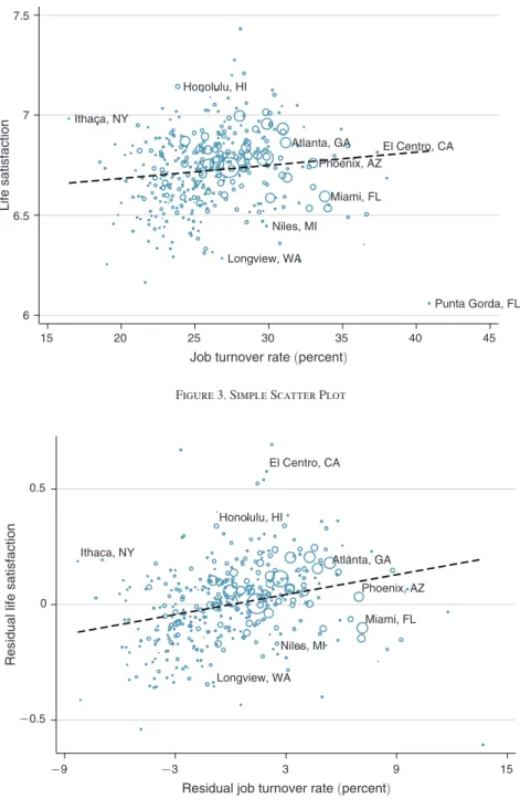
MSA-Level Results.—Before displaying the regression results, we show two scat-ter plots where one observation corresponds to an MSA. Figure 3 plots the MSA’s average life satisfaction on MSA-level job turnover, where circle sizes are propor-tional to MSA population levels. We then regress these MSA-level life satisfaction and job turnover variables on the MSA’s unemployment rate and plot the residuals in Figure 4. We see that well-being is more strongly positively associated with job turnover, once we control for the unemployment rate.

Figure 3. Simple Scatter Plot

Atlanta, GA _{El Centro, CA} Honolulu, HI Ithaca, NY Longview, WA Miami, FL Niles, MI Phoenix, AZ Punta Gorda, FL 6 6.5 7 7.5 Life satisfaction 15 20 25 30 35 40 45

Job turnover rate (percent)

Atlanta, GA El Centro, CA Honolulu, HI Ithaca, NY Longview, WA Miami, FL Niles, MI Phoenix, AZ −0.5 0 0.5

Residual life satisfaction

−9 −3 3 9 15

Residual job turnover rate (percent) Figure 4. Residual Scatter Plot

Now moving to the regression results, Table 2, panel A, shows the results from baseline OLS regressions at the MSA level. We see that job turnover has a positive but statistically insignificant effect on current well-being. Column 2 shows that once we control for unemployment, job turnover has an effect on well-being that is more than twice as large and strongly statistically significant. This is in line with our model which predicts that, controlling for unemployment, turnover should have a more positive effect on well-being as it implies higher growth and a higher probability for currently unemployed workers of finding a new job.19 _{In column 3, we add}

addi-tional MSA controls: population, crime rate, and share of African Americans.20 _We

see that these potential confounders do not significantly affect the coefficients of the creative destruction variable.

The difference between the estimates on creative destruction in column 1 ver-sus 2 and 3 is statistically significant at the 1 percent level. The last row in each panel of Table 2 reports the p-value associated with a Wald test of the hypothesis that _{α CD;column1 = α CD;column2 .}

Column 4 repeats the same specification as column 3 but with future well-being as the dependent variable. We first see that job turnover has a stronger effect on the future ladder than on the current Cantril ladder. This in turn points to the notion that individuals disentangle the short-run losses from becoming unemployed as a result of job turnover from the long-term gains associated with higher growth and more new job opportunities in the future.

The magnitude of the effect of creative destruction on current life satisfaction is in the same ballpark as that of the effect of the unemployment rate. In particular, moving from an MSA which is at the twenty-fifth percentile in terms of its level of creative destruction _{(i.e., with a job creation rate + destruction rate at 23.5 percent)} to an MSA at the seventy-fifth percentile (i.e., with a job creation rate plus job destruction rate at 28.3 percent_{) is associated with an increase in the current ladder} of life of 0.06 points (column 2 in Table 2, panel A). As a benchmark, looking at the same regression, moving from the seventy-fifth to the twenty-fifth percentile in terms of the unemployment rate (that is, from a 9.4 percent to a 6.7 percent unemploy-ment rate_{) is associated with an increase in life satisfaction of 0.07 points. Another} way to put it is that a one standard deviation increase in job turnover increases the current ladder by 0.25 standard deviation: that effect is equivalent to a 0.7

(

)

Individual-Level Results.—In Table 2, panel B, we perform individual-level regressions and find qualitatively similar results as in panel A. The difference is that we now also control for individual-level characteristics and for year and month fixed effects. We thus control for household income brackets and we keep the control for the MSA-level log of income. Note that the MSA-level income has a negative impact on well-being once we control for individual-level income, which suggests 19 _{The correlation between the MSA-level average job turnover rates over the period 2008–2011 and the} MSA-level average unemployment rates over the same period, is equal to 0.344.

20 _{The share of African Americans is a weighted average of the number of respondents in the surveys that report} being black in the race question. Weights used to compute the weighted average are those attached to the respondent by Gallup.

Table 2—Test of Prediction 1

Current ladder Future ladder

(1) (2) (3) (4)

Panel A. MSA-level analysis

Job turnover rate 0.599 1.288 1.322 1.726

(0.361) (0.410) (0.424) (0.306)

Unemployment rate −2.727 −2.581 −0.930

(0.786) (0.823) (0.507)

log of income 0.342 0.195 0.225 0.297

(0.0839) (0.088) (0.106) (0.079)

Additional MSA controls x x

Observations 363 363 344 344

R2 _{0.100 0.198 0.217 0.459}

p-value job turnover _{[1] = job turnover [2]} 0.000

Panel B. Individual-level analysis

Job turnover rate 0.0676 0.521 0.611 0.984

(0.236) (0.237) (0.285) (0.148)

Unemployment rate _{−2.299 −2.168 −0.0857}

(0.443) (0.502) (0.298)

MSA-level log of income −0.187 −0.285 −0.263 −0.0424

(0.048) (0.046) (0.051) (0.038)

Additional MSA controls x x

Individual controls (incl. income) x x x x

Year and month fixed effects x x x x

Observations 556,300 556,300 461,054 450,908

R2 _{0.103 0.104 0.103 0.095}

p-value job turnover [1] = job turnover [2] 0.000

Panel C. Panel analysis

Job turnover rate 0.678 0.787 0.249 0.234

(0.0970) (0.105) (0.142) (0.140)

Unemployment rate −2.238 −1.743 −1.074

(0.301) (1.054) (1.057)

log of income 0.410 0.360 0.412 0.192

(0.0301) (0.0307) (0.0373) (0.0390)

MSA fixed effects x x

Additional MSA controls x x x x

Year and quarter fixed effects x x x x

Observations 4,884 4,884 4,884 4,884

R2 _{0.189 0.203 0.325 0.256}

p-value job turnover _{[1] = job turnover [2]} 0.041

Notes: The dependent variables are SWB measures from Gallup: columns 1 through 3 use the current Cantril lad-der of life whereas column 4 uses the future ladlad-der of life. Sample years are 2008–2011 and the sample is restricted to working-age respondents. Column 1 regresses SWB on the job turnover rate, which comes in panels A and B, from the BDS, and in panel C, from the LEHD which provide data at the quarterly level. Column 2 adds a control for the MSA-level unemployment rate. Columns 3 and 4 further add some MSA-level controls: population (in lev-els), crime rates, and share of African Americans. All specifications control for income at the MSA-level. All data sources and variable definitions are in the main text. Panel A carries a cross-sectional analysis at the MSA-level, where the variables are averaged across years within each MSA. The SWB measures are averaged using the weights attached by Gallup to each respondent. Panel B carries a repeated cross-section analysis at the individual-level. Month and Year fixed effects are added to the specification as well as individual controls: age, age squared, a dummy for being female, six dummies for family status, six dummies for education, and four race dummies (black, Asian, white, other, or missing), as well as nine dummies for household income brackets. Regressions are weighted by individual weights attached by Gallup to each respondent. Panel C shows the results of a quarterly panel analysis at the MSA-level. The SWB measures are averaged at the MSA-quarter level using the weights attached by Gallup to each respondent. All regressions include year and quarter fixed effects, quarterly controls for the MSA’s average log of income, and the share of African Americans in the MSA, as well as annual controls for population levels and crime rates. Columns 3 and 4 add MSA fixed effects.

that well-being depends on relative income of an individual. The creative destruc-tion variable now varies at the MSA-year level.

We can still reject at the 1 percent level that the coefficient of job turnover on well-being is the same whether or not we control for the unemployment rate. We also see that the effect of turnover is stronger on the future ladder than on the current ladder.

The magnitude of the creative destruction effect is smaller than that displayed at the MSA level. A one standard deviation increase in job turnover has an effect on the current ladder of life which is equivalent to a 0.3 standard deviation increase in the MSA-level unemployment rate

(

)

Panel Results.—In panel C, we show results from quarterly panel regressions with year and quarter fixed effects, with and without MSA fixed effects. However, we want to stress why we have a preference for the cross-sectional analysis. The theoretical concept of creative destruction is being proxied in our empirical analysis by a job turnover variable. So we are proxying x(t) by x ∗ (t) which is equal to x(t) plus some measurement _{(or proxy) error ϵ(t) . Adding MSA fixed effects into the} regression changes in an unfavorable way the relative variances of the signal, the variance of x_{(t) , and the noise, the variance of ϵ(t) . If the job destruction variable} changes only slowly over time within each MSA, which is the case here, looking at the deviation of job destruction from its MSA time-mean is going to be problematic, as more of that deviation is going to come from the proxy error, not from the vari-able itself. Hence our predictions are better captured by cross-sectional regressions than by panel regressions that cover such short time periods.

Because our sample period is very short, we use a quarterly frequency to look at panel specifications. Thus we use the LEHD dataset constructed by the Census Bureau, based on the Quarterly Census of Employment and Wages and other administrative and survey data. Indeed, these data contain information on employment, earnings, and job flows at the MSA and quarterly level. In terms of creative destruction: rather than job creations and destructions, the data give us the number of hires and separations. To compute the turnover rates, we divide these hires or separations by the average stock of employment in that quarter. The results are reported in Table 2, panel C.

If we compare column 1 to column 2, we see again that the coefficient for job turn-over is higher when we control for the MSA-level unemployment rate than when we do not. The difference is significant at the 5 percent level. These two columns are with-out MSA fixed effects. When we add MSA fixed effects (column 3), the coefficient of job turnover is still significantly positive at the ten percent level, although of a smaller magnitude. Note that all the specifications in panel C control for time-varying poten-tial MSA-level controls: population levels, crime rates, share of African Americans.

D. Testing Prediction 2

In this section, we test Prediction 2: A higher job creation rate increases

well-be-ing, whereas a higher job destruction rate decreases well-being.

MSA-Level Results.—Table 3, panel A, shows the results from the baseline OLS regressions at the MSA level. The first two columns use current ladder whereas

Table 3—Test of Prediction 2

Current ladder Future ladder

(1) (2) (3) (4)

Panel A. MSA-level analysis

Job creation rate 5.486 5.567 3.588 3.103

(0.978) (1.015) (0.825) (0.682)

Job destruction rate _{−3.586 −3.433 −0.158} 0.144

(0.838) (0.870) (0.702) (0.668)

log of income 0.277 0.293 0.221 0.324

(0.077) (0.094) (0.061) (0.073)

Additional MSA controls x x

Observations 363 344 363 344

R2 _{0.218 0.246 0.149 0.460}

Panel B. Individual-level analysis

Job creation rate 1.098 1.274 1.068 0.944

(0.395) (0.445) (0.206) (0.220)

Job destruction rate _{−0.791 −0.702} 0.926 0.987

(0.274) (0.306) (0.197) (0.225)

MSA log of income −0.197 −0.173 −0.0408 −0.0382

(0.046) (0.048) (0.031) (0.038)

Additional MSA controls x x

Individual controls (incl. income) x x x x

Year and month fixed effects x x x x

Observations 556,300 461,054 544,228 450,908

R2 _{0.103 0.103 0.094 0.095}

Panel C. Panel analysis

Job creation rate 2.276 1.213 1.690 1.155

(0.316) (0.357) (0.293) (0.349)

Job destruction rate _{−0.617 −0.466 −0.647 −0.460}

(0.274) (0.314) (0.249) (0.285)

log of income 0.416 0.416 0.266 0.195

(0.0299) (0.0371) (0.0304) (0.0389)

MSA fixed effects x x

Additional MSA controls x x x x

Year and quarter fixed effects x x x x

Observations 4,884 4,884 4,884 4,884

R2 _{0.195 0.325 0.145 0.257}

Notes: The dependent variables are SWB measures from Gallup: columns 1 and 2 use the current Cantril ladder of life whereas columns 3 and 4 use the future ladder of life. Sample years are 2008–2011 and the sample is restricted to working-age respondents. Columns 1 and 3 regress these life satisfaction measures on the job creation and the job destruction rates, which come, in panel A and B, from the BDS, and in panel C, from the LEHD which provide data at the quarterly level. All specifications control for income at the level. Columns 2 and 4 add some MSA-level controls: the unemployment rate, population (in levels), crime rates, and share of African Americans. All data sources and variables definitions are in the main text. Panel A carries a cross-sectional analysis at the MSA-level, where the variables are averaged across years within each MSA. The SWB measures are averaged using the weights attached by Gallup to each respondent. Panel B carries a repeated cross-section analysis at the individual-level. Month and Year fixed effects are added to the specification as well as individual controls: age, age squared, a dummy for being female, six dummies for family status, six dummies for education, and four race dummies (black, Asian, white, other, or missing), as well as nine dummies for household income brackets. Regressions are weighted by individual weights attached by Gallup to each respondent. Panel C shows the results of a quarterly panel analysis at the MSA level. The SWB measures are averaged at the MSA-quarter level using the weights attached by Gallup to each respondent. All regressions include year and quarter fixed effects, quarterly controls for the MSA’s average log of income, and the share of African Americans in the MSA, as well as annual controls for population levels and crime rates. Columns 2 and 4 add MSA fixed effects.

the last two columns use the future ladder as dependent variables. In the first and third columns, we see the positive effect of job creation and the negative effect of job destruction on current and future well-being which are very much in line with Prediction 2. Columns 2 and 4 introduce additional MSA-level confounders: the MSA’s average population level over the period, its average crime rate and its average share of African Americans. These controls do not change the pattern: over-all, job creation and destruction have opposite effects on well-being, as the theory predicted.

Now, consider the magnitudes of the various effects. A one standard deviation increase in the job creation rate is associated with an increase in the current ladder of life of slightly more than half a standard deviation

(

)

(

)

Individual-Level Results.—In Table 3, panel B, we perform individual-level regres-sions and find qualitatively similar results as in panel A. Again, we control for many demographic characteristics as well as income brackets. All specifications include year and month fixed effects as well as a control for the MSA’s log of income. The job creation and destruction rates vary at the MSA-year level. Standard errors are clus-tered at the MSA level. Again, columns 2 and 4 are similar to columns 1 and 3 except that additional MSA-level potential confounders are added. We see that these addi-tional controls barely change the coefficient on the job creation and destruction rates. Similar to Prediction 1, the magnitudes are smaller than for the MSA-level results.

Panel Results.—In panel C, we show results of panel specifications using quar-terly data on job creation and destruction rates coming from the LEHD, as in panel C of Table 2. Columns 1 and 3 are without MSA fixed effects, whereas col-umns 2 and 4 are with MSA fixed effects. All specifications include year and quarter fixed effects as well as MSA-level potential confounders such as share of African Americans, population level, and crime rate. Prediction 2 remains verified in panel analysis, with a positive effect of the job creation rate on SWB and a negative effect of the job destruction rate.

E. Testing Prediction 3

In this section, we test Prediction 3: A higher turnover rate increases well-being

more, whereas a higher job destruction rate decreases well-being less, the more

generous the unemployment benefits.

The generosity of unemployment insurance _{(UI) varies at the state level. To avoid} the endogeneity of the total number of benefits claimed, we use, as is standard in the literature, the maximum weekly benefit amount as a measure of the state’s UI generosity. We normalize it by the average taxable wage. Our results are robust to whether or not we do this normalization. Panel A of Table 4 carries the analysis at the MSA-level whereas panel B shows the results when using individual level regressions, controlling for the same individual characteristics used in panel B of Tables 2 and 3. The coefficients of interest are that of the interaction term between job turnover and UI generosity, as well as that of the interaction term between job

destruction and UI generosity. Indeed we expect the effect of UI generosity to alle-viate the negative effect of the job destruction rate by making the risk of unemploy-ment less costly. On the contrary, there is no clear prediction on how UI generosity should interact with the job creation rate. Thus we do not report the interaction terms and main effect of the job creation rate although these variables are included in all the specifications that feature the job destruction rate _{(i.e., columns 3 and 4). Note} that we demean our measure of the state’s UI generosity such that the coefficients for the main effect of the job turnover or the job destruction rate show the effect for MSAs located in a state where the UI generosity is at its mean value.

MSA-Level Results.—We see that the effect of the job turnover rate on SWB at the mean value of UI generosity is positive and that the coefficient of the interaction

Table 4—Test of Prediction 3

Current ladder

(1) (2) (3) (4)

Panel A. MSA-level analysis

Job turnover rate 0.524 0.662

(0.362) (0.378)

Job turnover _{× UI generosity} 0.989 0.897

(0.422) (0.416)

Job destruction rate −3.661 −3.536

(0.789) (0.816)

Job destruction _{× UI generosity} 2.357 2.369

(1.105) (1.113)

UI generosity −0.288 −0.253 −0.167 −0.137

(0.114) (0.113) (0.128) (0.128)

Additional MSA controls x x

Observations 363 344 363 344

R2 _{0.116 0.136 0.237 0.262}

Panel B. Individual-level analysis

Job turnover rate 0.0845 0.209

(0.230) (0.262)

Job turnover _{× UI generosity} 0.675 0.670

(0.310) (0.357)

Job destruction rate −0.794 −0.720

(0.272) (0.300)

Job destruction _{× UI generosity} 0.620 0.673

(0.329) (0.372)

UI generosity −0.198 −0.183 −0.212 −0.200

(0.085) (0.096) (0.083) (0.094)

Individual controls _{(incl. income)} x x x x

Year and month fixed effects x x x x

Additional MSA controls x x

Observations 556,300 461,054 556,300 461,054

R2 _{0.103 0.103 0.104 0.103}

Notes: Panel A carries a cross-sectional analysis at the MSA-level, where the variables are averaged across years within each MSA, whereas panel B carries a repeated cross-section analysis at the individual-level. The first two columns are similar to the columns 1 and 3 of Table 2, and the last two columns are similar to the first two col-umns of Table 3, except that the creative destruction variables ( job turnover, job creation, and destruction rates) are interacted with state-level UI generosity. UI generosity is measured by the average maximum weekly benefit amount over the period 2008–2011 normalized by the average taxable wage in covered employment. The variable is demeaned. We don’t report the interaction coefficient for job creation as the interaction of interest is the job destruc-tion one (see main text).