Analysis of crystallographic texture information by the hyperspherical harmonic expansion

(1)

Analysis of Crystallographic Texture Information by the Hyperspherical Harmonic Expansion

by

MASSACHUSETTS INSTiTUTE OFTECHNOLOGY

Jeremy K. Mason OF TECHNOLOGY

S.B., Physics (2005)

JUL 2 8 2009

Massachusetts Institute of Technology

LIBRARIES

ARCHIVES Submitted to the Department of Materials Science and Engineering

in Partial Fulfillment of the Requirements for the Degree of Doctor of Philosophy in Materials Science and Engineering

at the

Massachusetts Institute of Technology June 2009

Signature of Author... ...

Department of Materials Stience and Engineering May 18, 2009

Certified by ...

Christopher Schuh Danae and Vasilios Salapatas Associate Professor of Metallurgy A Thesis Aupervisor A ccepted by ... .. ... .

Christine Ortiz Chair, Departmental Committee on Graduate Students

(2)

Analysis of Crystallographic Texture Information by the Hyperspherical Harmonic Expansion

by

Jeremy K. Mason

Submitted to the Department of Materials Science and Engineering on May 18, 2009 in Partial Fulfillment of the Requirements for the Degree of

Doctor of Philosophy in Materials Science and Engineering

Abstract

The field of texture analysis is fundamentally concerned with measuring and analyzing the distribution of crystalline orientations in a given polycrystalline material. Traditionally, the orientation distribution function describing crystallographic orientation information is written as a linear combination of the generalized spherical harmonics. Since the use of generalized spherical harmonics requires that orientations be described by sets of Euler angles, the field of texture analysis suffers from the inherent limitations of Euler angles. These include difficulty of presentation and interpretation, discontinuous changes in the description of a changing orientation, and singularities in many equations of Euler angles. An alternative expansion of the orientation distribution function as a linear combination of the hyperspherical harmonics is therefore proposed, with the advantage that this expansion allows rotations to be described by angles that directly relate to the axis and angle of a rotation. Apart from the straightforward and intuitive presentation of orientation statistics that this allows, the utility of the hyperspherical harmonic expansion rests on the fact that the orientation distribution function inherits the useful mathematical properties of the hyperspherical harmonics. The relationship of the hyperspherical harmonics to the three- and four-dimensional rotation groups is investigated, and expressions for the matrix elements of the irreducible representatives of these rotation groups as linear combinations of the hyperspherical harmonics are found. These expressions allow an addition formula for the hyperspherical harmonics to be derived, and provide the means to write a simple conversion between the generalized spherical harmonic and hyperspherical harmonic expansions. This allows results derived via the hyperspherical harmonic expansion to be related to the texture analysis literature. Furthermore, a procedure for calculating the symmetrized hyperspherical harmonics consistent with crystal and sample symmetries is indicated, and used to perform the expansion of an orientation distribution function significantly more efficiently. The capability of the hyperspherical harmonic expansion to provide results not traditionally accessible is demonstrated by the generalization of the Mackenzie distribution to arbitrary textures. Finally, further areas where the application of the hyperspherical harmonic expansion is expected to advance the field of texture analysis are discussed. Thesis Supervisor: Christopher Schuh

(3)

List of Figures

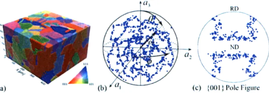
Figure 1: The progressive abstraction of microstructural information. (a) Three-dimensional reconstruction of the microstructure of a commercial austenitic stainless steel; reproduced from Figure 5 of Ref. [2], with kind permission of Springer Science and Business Media. (b) Axis-angle representation of the texture of a crystalline material, completely characterizing the crystallographic orientations present. (c) Stereographic projection indicating the orientation of {100} _{crystallographic planes of a material with a copper} texture.

Figure 2: Comparison of rotations performed in the active and passive conventions. (a) Rotations in the active convention. A vector u is rotated by ff2 about the z

axis to u', then by vz2 about the x axis to u". (b) Rotations in the passive

convention. The coordinate system is rotated by r/12 about the x axis, then by /2 about the z' axis. (c) Effect of the passive rotations in (b) on v from the viewpoint of an observer attached to the coordinate system. The vector v appears to be rotated by -7r12 about the x axis, then by -r1/2 about the z' axis. Figure 3: Indication of a crystallographic plane's orientation by a point on the surface

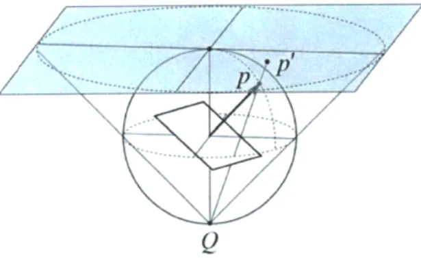
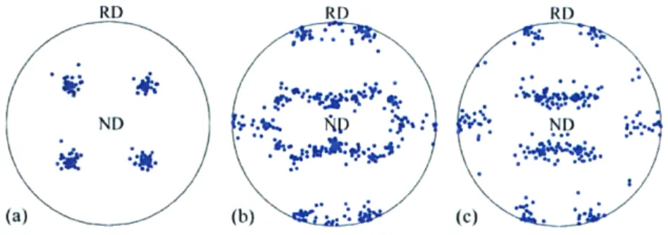
of a sphere, projected onto a plane by stereographic projection. The stereographic projection of a point p may be performed by placing a light source at Q and observing the shadow cast by the point p onto the plane at p'. Figure 4: _{{111 } pole figures for (a) a cube texture, (b) a copper texture, and (c) a brass} texture. _{"ND" and "RD" correspond to the "normal direction" and the} "rolling direction", respectively, of a sample deformed by rolling.

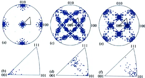
Figure 5: Normal-direction inverse pole figures for the three textures in Figure 4. The inverse pole figure at the top of a given column is divided into twenty-four stereographic triangles, with the standard stereographic triangle outlined. This triangle appears alone at the bottom of the column. Miller indices in the figure refer to directions in the local crystallographic frame. (a) A cube texture, and (b) the standard stereographic triangle of the cube texture. (c) A copper texture, and (d) the standard stereographic triangle of the copper texture. (e) A brass texture, and (f) the standard stereographic triangle of the

brass texture.

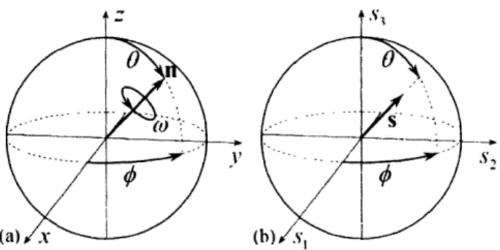
Figure 6: Relationship of the vector n and angle c to the parameters of a neo-Eulerian mapping. (a) The result of any series of rotations is equivalent to some rotation, performed about an axis parallel to n by an angle w. The vector n can be written in terms of the spherical angles 0 and 0. (b) The corresponding point in the group space of a neo-Eulerian mapping with parameters s = _{nf(wc). The result is nearly as straightforward to interpret as}

(6)

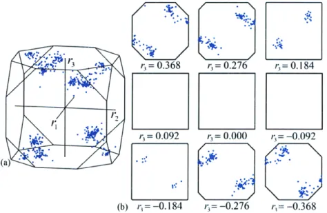
Figure 7: A collection of discrete orientations from a copper textured material with cubic crystal symmetry, depicted in the fundamental zone of Rodrigues space. (a) The cubic fundamental zone containing the origin is a truncated cube with six octagonal faces and eight triangular faces. (b) The distribution is conventionally plotted in equidistant sections perpendicular to the r3 axis. Figure 8: A collection of discrete orientations from a copper textured material with

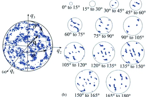
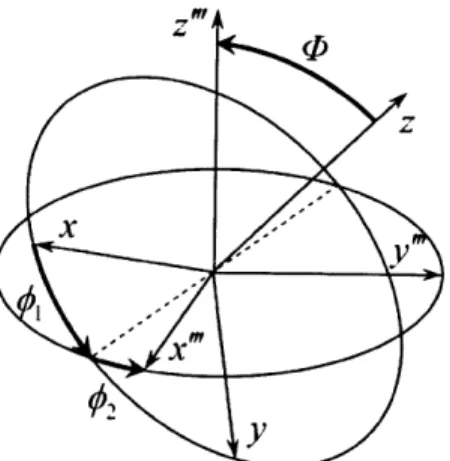
cubic crystal symmetry, depicted in (a) the three dimensions inhabited by the vector part q of a quaternion q, and (b) in two dimensions as a collection of stereographic projections of concentric spherical shells of the space in (a). This presentation is naturally suited to the spherical shape of the space, and has the advantage that the rotation angle is constant within a given spherical shell, promoting an intuitive interpretation of points displayed in this format. Figure 9: Definition of the orientation of a coordinate system, following the

conventional interpretation of the Euler angles. The orientation is determined as the result of three consecutive rotations, performed about z, x', and z" axes

by the angles 01, P, and 02, respectively.

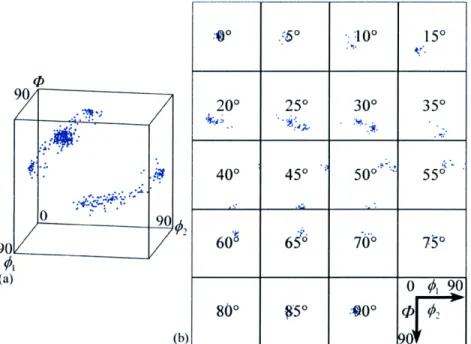
Figure 10: A collection of discrete orientations from a copper textured material with cubic crystal symmetry, depicted in Euler angle space. (a) The conventional volume used for cubic crystal symmetry and orthorhombic sample symmetry is bounded by planar surfaces, but contains three fundamental zones. (b) The distribution is conventionally plotted in equidistant sections perpendicular to the 0₂axis.

Figure 11: {1 11} _{pole figures of the continuous pole distributions for (a) a cube texture,}

(b) a copper texture, and (c) a brass texture, corresponding to the respective discrete pole figures in Figure 4. The distribution functions are determined by Equation (15), with Imax = 15. Regions of finite probability density appear in some areas that are empty in the corresponding discrete pole figures due to the use of a limited number of terms, while regions of negative probability density were removed by applying a positivity constraint.

Figure 12: Continuous Euler angle distribution for the crystal orientations in a copper textured material, corresponding to the collection of discrete orientations in Figure 10. The distribution function is determined by Equation (18), with Imax = 12. (a) A single contour of the distribution function in the conventional volume used for cubic crystal symmetry and orthorhombic sample symmetry. (b) The distribution function, sectioned perpendicular to the O2 axis. Regions of finite probability density appear in some areas that are empty in Figure 10b due to the use of a limited number of terms, while regions of negative probability density were removed by applying a positivity constraint.

Figure 13: Relationship shared by the axis-angle parameterization of a rotation, the quaternion parameterization of a rotation, and the parameterization of a quaternion by three angles. (a) A three-dimensional rotation by the angle Co about the unit vector n, pointing along the axis of rotation. The direction of n

(7)

is specified by the angles 0 and 4. (b) The vector part q of the quaternion q, corresponding to the rotation in (a). The vectors q and n point in the same direction, though the length of q is sin(o/2) rather than one.

Figure 14: Continuous quaternion distribution for the crystal orientations in a copper textured material, corresponding to the collection of discrete quaternions in Figure 8. The distribution function is determined by Equation (31), with

nmax = 24. (a) A single contour of the distribution function in the space of the vector part q of a quatemion q. (b) The distribution function, shown in two dimensions as stereographic projections of concentric spherical shells of the space in (a). Regions of finite probability density appear in some areas that are empty in Figure 8b due to the use of a limited number of terms, while regions of negative probability density were removed by applying a positivity constraint.

Figure 15: A random texture, corresponding to a uniform distribution of points on the surface of the unit four-dimensional sphere, presented using the volume-preserving (4D to 3D) and equal-area (3D to 2D) projections. The equal-area projection causes the uniformity of the distribution for a particular rotation angle, and the volume-preserving projection causes the uniformity of the distribution among the various rotation angles.

Figure 16: The physical interpretation and relationship of the quantities Tm'm

(10

, 2 D'm m ( ₁, gP, 4 2), and U,,

(,

0, ). Tn'm( , , 02 ) is considered to passively

bring the coordinate system into coincidence with an oriented crystal.

Dml,m(4,0 ( 2) is considered to actively bring an oriented crystal into coincidence with the coordinate system; this is identical to the effect of

Tm' (0, , 2 _{) from the perspective of an observer attached to the coordinate}

system. U'~,n (c, 0, ) is considered to actively bring a reference crystal into coincidence with the oriented crystal; this is the inverse of the effect of

Figure 17: The normal direction inverse pole figure of a copper sample, as measured experimentally by EBSD.

Figure 18: The ODF of the copper sample in Figure 17, expressed via the hyperspherical harmonic expansion given in Equation (96). Blue and red indicate regions of positive and negative probability density, respectively. (a) The coefficients of the expansion are calculated using Equation (97). (b) The coefficients of the expansion are calculated using Equations (95) and (122), i.e. by means of the coefficient conversion formulas. Inspection of the figures reveals that the expansions are identical.

Figure 19: The ODF given in Figure 18a, constrained to positive values by the procedure described in Section 4.6. Apart from the removal of the regions of negative probability density and a slight broadening of the peaks, the distribution function is identical.

(8)

Figure 20: An example of the reduction in the number of linearly independent harmonics required for the expansion of a function on the surface of a sphere with cubic point group symmetry; blue and red correspond to positive and negative values respectively. (a) The nine spherical harmonics defined by Equation (14) for 1 = 4. The value of the index m is indicated above the columns, with the harmonics Y,'"c on the top and Y,'"' on the bottom of a given column. (b) The single linear combination of the harmonics in (a) that satisfies the requirements of cubic point group symmetry.

Figure 21: Examples of the symmetrized hyperspherical harmonics, as calculated from the tables of coefficients in Appendix E. Specifically, these are sets of the three lowest-order, non-trivial symmetrized hyperspherical harmonics for orthorhombic sample symmetry and for the crystal point symmetries (a) 222, (b) 422, and (c) 432. In each of the projections, the z and x axes of the projections point out of the page and to the right, respectively.

Figure 22: Conventional methods of viewing a simulated cube texture. (a) The (100) and (b) (111) pole figures are presented in stereographic projection, with the z

and x axes pointing out of the page and up the page, respectively. (c) The blue and red regions in the Euler angle space indicate regions of positive and negative probability density, respectively.

Figure 23: The current method of viewing a simulated cube texture. The z and x axes of the projections point out of the page and to the right, respectively. (a) Projection of the discrete quaternions corresponding to the simulated texture, including all of the rotations in the crystallographic point group 432. (b) ODF corresponding to the discrete distribution of part (a), calculated using the first thirty-seven hyperspherical harmonics of orthorhombic sample symmetry and cubic crystal symmetry. Blue and red regions indicate regions of positive and negative probability density, respectively.

Figure 24: Conventional methods of viewing a simulated copper texture. (a) The (100) and (b) (1 11) pole figures are presented in stereographic projection, with the z

and x axes pointing out of the page and up the page, respectively. (c) The blue and red regions in the Euler angle space indicate regions of positive and negative probability density, respectively.

Figure 25: The current method of viewing a simulated copper texture. The z and x axes of the projections point out of the page and to the right, respectively. (a) Projection of the discrete quaternions corresponding to the simulated texture, including all of the orientations described in Ref. [89]. (b) ODF corresponding to the discrete distribution of part (a), calculated using the first thirty-seven hyperspherical harmonics of orthorhombic sample symmetry and cubic crystal symmetry. Blue and red regions indicate regions of positive and negative probability density, respectively.

Figure 26: The cubic orientation (light lines) and disorientation (bold lines) spaces, displayed in the orthographic projection of the quaternion space. The solid

(9)

points mark the intersection of the axes with the surface of the orientation space. The q, are the components of the vector part of the quaternion.

Figure 27: {100} pole figure plots for simulated cube textures of varying degrees of sharpness, plotted in equal area projection. The angles indicate the maximum allowed disorientation angle of a cubic crystal from the reference orientation. The normal direction is out of the page, and the rolling direction is vertical in the plane of the page.

Figure 28: Disorientation angle distribution functions corresponding to simulated cube textures of varying degrees of sharpness (cf. Figure 27). Labels given in degrees indicate the maximum allowed disorientation angle of a cubic crystal from the reference orientation (smaller values denote sharper textures), while the heavy dark line corresponds to a material in which every misorientation is equally likely.

Figure 29: Disorientation angle distribution function for a copper texture, assuming the absence of correlations relating the orientations of neighboring grains or relating the orientation and shape of a single grain. The solid line is the result of our simulation, while the bars indicate the probability density for an experimental material with a similar texture, as measured by Mishin, Gertsman and Gottstein [106]. The dashed line corresponds to a material in which every misorientation is equally likely (i.e., the Mackenzie distribution). Figure 30: Representative triple junction depicting the physical significance of the quantities co and #. Grain A is rotated by the angle oA and is located opposite the boundary with orientation #A; a similar geometry applies for grains B and C.

Figure 31: Comparison of the quantities used to define the state of a grain boundary. A single boundary is depicted in terms of (a) co, co' and # and (b) 0 and p. Notice that in (b) the grains share the misorientation equally, resulting from a rotation of the system in (a).

Figure 32: Labeling scheme for the grain rotations o and the quantities Oand p around a triple junction. The misorientations 0 are the rotations that bring the grain at the tail of the arrow into coincidence with the grain at the head. Our labeling scheme differs in sense from some similar examples in the literature [97]. Figure 33: Lattices of symmetrically equivalent points and corresponding unit cells for 0

and (p at a single grain boundary. (a) 0 and p display independent periodicities of ao and co/2, respectively, resulting in a rectangular lattice and simply described boundaries. (b) 0 and p display joint periodicities, leading to a sparser lattice, an extended range of unique quantity pairs, and more complicated boundaries.

Figure 34: Lattices of symmetrically equivalent points and corresponding unit cells for OA, OB and Oc at a triple junction. (a) OA, 8B and Oc each display independent periodicities of co, resulting in a cubic lattice. The size of the markers indicates the relative positions of points residing in the three (111) type

(10)

planes shown. (b) The three misorientations display joint periodicities, such that the lattice resides entirely in the (111) plane and each lattice point

satisfies the constraint OA + OB + 0. = 0.

Figure 35: Representation of the distribution functions for misorientations about a triple junction. Triple junctions are classified by the number of misorientations smaller in magnitude than O; for this figure, 0 9, < w, /3. Darker shading corresponds to more special boundaries, e.g., white is a Jo region, and dark grey is a J3 region. Solid lines indicate unit cell borders in the current representation, and dashed lines in the alternate representation. (a) Classification of triple junctions as defined by Equation (211). For clarity of representation, the distribution is projected into the plane spanned by OA and 0B. This representation is preferred for integration due to the simplicity of the equations of the region boundaries. (b) Classification of the triple junction distribution defined by Equation (209). Bands of special boundaries occur in a high symmetry configuration, and classification is continued outside of the fundamental zone to emphasize this symmetry. The three regions in dashed lines correspond to the three parallel planes that intersect the unit cell appearing in Figure 34a.

Figure 36: Analytic solutions for the special fraction of boundaries in correlated boundary networks, for the specific case where w is uniformly distributed on

the interval - omax : o < Imax , and 0, = o, /6 with cos the angle of rotational

symmetry of the crystallites. Our exact solution (Equation (213)) is given by the solid black line, and is valid over the full range of Cmax

/w,

. The vertical

dashed lines appear at omax = 9,/2 and cm,ax = O, /2 - 9, /2. The solutions

of Frary and Schuh [97] and Van Siclen [98] are represented by the dashed grey line, which deviates for cmnax < , /2 and excludes the effects of crystal symmetry for co, /2 - O,/2 < oma, . A further result for Omax = O, /2, found

by Van Siclen, is denoted by the black dot. Equation (222), our simplification for sharp textures, is shown by the series of grey points.

Figure 37: Triple junction fractions plotted as a function of the special boundary fraction in correlated boundary networks, for the specific case where co is distributed

uniformly on the interval - omwax c < wmnax. For comparison, the dotted

lines show the predicted triple junction fractions for a random (uncorrelated) spatial distribution of misorientations. Solutions by Frary and Schuh [97]

and Van Siclen [98] for cwmax < c, /2 - , /2 appear as the solid lines, and the specific case derived by Van Siclen for cOnax = Cs /2 is given by the dashed lines. Our solutions, presented in Appendix I, migrate continuously over the regions shaded in grey with changes in the values of co, and O.

(11)

1. State of the Field'

The field of materials science and engineering is fundamentally concerned with manipulating the microstructure of materials in order to control their properties. Recent improvements in instrumentation, which include electron backscatter diffraction (EBSD), dramatically enhance our abilities in this regard by providing extensive crystallographic orientation information of a given two-dimensional section of a microstructure. As this technique has been developed and combined with chemical analysis and serial sectioning methods, it has become possible to access complete three-dimensional chemistry, phase, and crystal orientation information; in short, the microstructural state of a polycrystal may now be completely quantified.

While these techniques allow an unprecedented opportunity for examining the microstructure-property relationships of materials, in many cases the controlling physics depend on only a relatively small subset of the available information. For example, a variety of the effective tensor properties of materials (e.g. elasticity and transport coefficients) as well as inherently anisotropic, nonlinear properties at the single crystal level (e.g. plasticity and cracking) are governed primarily by the crystallographic texture, or the distribution of crystal orientations within a polycrystal. When properties of this type are of interest, it may be reasonable to simplify the analysis of a material by neglecting the spatial information of the microstructure and examining only the orientations of the crystalline grains.

Figure 1 illustrates schematically the process of abstraction that is useful when studying texture and the effects of texture on material properties. Figure la shows a complete microstructure, reconstructed from a progression of EBSD maps obtained through serial sectioning, where each grain is colored differently according to its orientation. The central purpose of texture representation is to preferentially examine the orientation of the crystallites without concern for their spatial characteristics, e.g. their arrangement, size and morphology; to this end, Figure lb shows a schematic representation of the distribution of discrete orientations sampled from the polycrystal. Numerous alternatives exist for the representation of texture information, and these will

(12)

& 'T ND

(a) (b) i (c) 0011 Pole Figure

Figure 1: The progressive abstraction of microstructural information. (a) Three-dimensional reconstruction of the microstructure of a commercial austenitic stainless steel; reproduced from Figure 5 of Ref. [2], with kind permission of Springer Science and Business Media. (b) Axis-angle representation

of the texture of a crystalline material, completely characterizing the crystallographic orientations present. (c) Stereographic projection indicating the orientation of {100} crystallographic planes of a material with a copper texture.

be covered at length later in this chapter. However, all of these alternatives, including that used in Figure lb, significantly distill the dataset represented by Figure la. Even more selective presentation of texture information is not only sometimes feasible, but may be necessary; in certain situations, only a portion of the orientation information is relevant or readily accessible. For example, many properties depend predominantly on the orientation of a single crystallographic axis, as for the c axis in transversely isotropic crystals. The representation of these crystallographic axes, or poles, is illustrated in Figure Ic.

The paradigm of data reduction and distillation exemplified in Figure 1 is not only powerful, but necessary. The acquisition of increasing amounts of data, in and of itself, does not provide the insights that advance the field. These insights depend entirely upon the depth of our understanding, and therefore on the skillful and judicious refinement of the data to a form that is both transparent and useful. Unfortunately, as with many unintuitive subjects, the essential content may be unintentionally obscured, or even discarded, during the process of simplification; in the case of crystallographic texture, it is altogether too easy to abandon the most critical information in the interest of depicting the data in a familiar form.

We explore the abstractions of Figure 1 in this chapter, both in a general sense and with specific emphasis on forms common in the materials science community. Since

(13)

this chapter is intended as an overview of a complex and well-developed field, the reader is referred to various works in the literature for more complete mathematical treatments as the need arises, e.g., Morawiec [3] and Bunge [4].

1.1. Rotations and Orientations

EBSD measures the discrete crystallographic orientations of volume elements arranged in a regular manner on the surface of a material. The analysis of material texture therefore begins with an examination of the available methods to parameterize discrete crystallite orientations and present the accumulated orientation information in a clear and concise format. Of course, this requires the definition of an orientation, which in turn requires the definition of a rotation.

.1.1. Defining a Rotation

While often not appreciated, a certain amount of precision is necessary in the definition of a rotation to be able to relate the rotation to the orientation of a particular object. For example, we may be provided with a rotation matrix, but unless the quantity on which the matrix acts and a method for applying the matrix are specified, the resulting orientation is obscured. One difficulty is that two conventions for defining a rotation appear in the literature, known as the active and passive conventions.

An active rotation is defined as a transformation of space relative to a stationary coordinate system. A rotation B then brings the vector u to the vector u', which is found to by left multiplying the column vector of the coordinates of u by a suitable matrix B:

u' = Bu. ₍₁₎

A second rotation of space A with respect to the same, stationary coordinate system similarly brings the vector u' to the vector u", found by left multiplying the coordinates of the vector u' with a suitable matrix A:

u"= Au'= ABu. (2)

By the associativity of matrix multiplication, the combined effect of these rotations on the vector u may instead be expressed as a left multiplication of u by the single matrix AB; that is, the combined effect AB of two rotations, B and A, is still a rotation.

(14)

A rotation in the passive convention behaves rather differently, by leaving the space fixed and rotating the coordinate system by which points are identified. For an observer attached to the rotating coordinate system, space appears to rotate in the reverse sense to that of the active convention. For example, perform the same rotation B as above, but on the coordinate system rather than on the space. Then the coordinates of the stationary vector v, relative to the rotated coordinate system, become

v' = B-'v, (3)

the matrix B-' performing the inverse operation of B. This result is generalized to the following relationship: the matrix transforming the coordinates of a vector during a passive rotation is the inverse of the matrix transforming the coordinates of a vector during the corresponding active rotation. The rotation AB that transforms coordinates by the matrix AB in the active convention, then, transforms coordinates by the matrix (AB)- = B-'A-' when interpreted in the passive convention; not only the sense of the individual rotations is reversed, but the order of application is reversed as well.

The difference between these conventions is demonstrated in Figure 2. The active convention is used in Figure 2a, where a vector initially on the x axis is aligned with the z

axis by a rotation of ;r/2 about the z axis and a rotation of ;r/2 about the x axis. The equivalent operation to that in Figure 2a is performed in the passive convention in Figure 2b by applying the individual rotations to the coordinate system in the same sense, but

A I #1

,U -

-u

----(a)/x (b) x, x' (c) x"

Figure 2: Comparison of rotations performed in the active and passive conventions. (a) Rotations in the active convention. A vector u is rotated by r/2 about the z axis to u', then by r/2 about the x axis to u". (b) Rotations in the passive convention. The coordinate system is rotated by //2 about the

x axis, then by r/2 about the z' axis. (c) Effect of the passive rotations in (b) on v from the viewpoint of an observer attached to the coordinate system. The vector v appears to be rotated by

(15)

reversed in order; the coordinate system is rotated by n/2 about the x axis, then by n-/2 about the resulting z' axis. This operation is equivalent to that in Figure 2a in the sense that the space in Figure 2a and the coordinate system in Figure 2b experience the same effective rotation by 2r/3 about the [1 11] direction. Figure 2c demonstrates that from the viewpoint of an observer attached to the coordinate system, the apparent rotation in Figure 2b is exactly the inverse, namely, a rotation by -2d/3 about the [1 1 ] direction.

While equivalent in the sense that one may be transformed into the other, the interpretation of matrices expressed in these conventions is clearly different. The convention used must therefore be clearly specified for a discussion of rotations to be meaningful. We use the active convention in the majority of the present work, for the reason that we find it simpler to interpret a rotation performed relative to a stationary frame of reference than a rotation performed with respect to a frame of reference that changes with every operation.

1.1.2. Defining an Orientation

An orientation is simply the physical result of a sequence of rotations. Rotations must be performed with respect to a coordinate system, usually defined as that system with coordinate axes aligned along the edges (often assumed to be orthogonal) of the sample being examined. The orientation of a crystal is identified with an active rotation that brings a reference crystal aligned with the coordinate system into coincidence with the crystal embedded in the material. The matrix corresponding to this rotation is designated by O, though there could be many equivalent such rotations. For example, the configuration resulting from an active rotation of a crystal by )r/2 about the z axis is equivalent to that resulting from a rotation by 57d2 about the same axis. Some of this redundancy is eliminated by considering only rotations by angles between 0 and r, but there is additional ambiguity that depends on the symmetries of the system.

A reference crystal with cubic symmetry could be initially aligned with the coordinate system in any of twenty-four physically indistinguishable ways. Indicating the symmetry operations of the crystallographic point group by C, all of the matrices OC, describe equivalent orientations of the crystal. Furthermore, the sample often exhibits

(16)

statistical symmetry in the distribution of crystal orientations as a result of processing history. When this symmetry is present, any of the symmetry operations S, can be applied to the sample without changing the observable characteristics, thereby expanding the set of rotations resulting in physically indistinguishable orientations to S,OC. A reasonable discussion of texture requires that an orientation be uniquely identified with just one of these rotations; usually, selecting the rotation with the minimum rotation angle about an axis lying in the standard stereographic triangle is sufficient. A discussion of more subtle cases, where this criterion does not uniquely identify the rotation, is given

elsewhere [5].

1.2. Pole Figures

One of the conventional methods for representing a texture is by means of pole figures. These originated as a natural result of diffraction experiments, and reveal the orientations of particular crystallographic planes rather than of individual crystals. Despite the development of more sophisticated methods of texture representation, the use of pole figures persists for a number of reasons; these include the familiarity of the materials science community with this method of presentation, the relative simplicity of physically interpreting the information displayed in this format, and the existence of many situations in which the orientation of a particular crystallographic plane controls some property of interest.

The orientation of a particular crystallographic plane is completely specified by a single line, passing through the origin and oriented in the direction normal to the plane. This line intersects a unit sphere centered on the origin in two diametrically opposed points. Since the line passes through the origin, either one of these two points uniquely identifies the line. The orientation of a single crystallographic plane is then completely specified by the point of intersection of the normal vector to the plane with the positive hemisphere of the unit sphere; this point is referred to as the pole. (Incidentally, the pole is identical to the crystallographic axis with the same indices for cubic crystals). An example of a pole, p, corresponding to a given plane orientation is shown in Figure 3.

When the poles of a particular crystallographic plane are considered, and the hemisphere is projected into two dimensions, a pole figure is obtained. The most

(17)

Figure 3: Indication of a crystallographic plane's orientation by a point on the surface of a sphere, projected

onto a plane by stereographic projection. The stereographic projection of a point p may be performed by placing a light source at Q and observing the shadow cast by the point p onto the plane at p'.

common projection for this purpose is the stereographic projection, which preserves angles but not area; the angle between two lines drawn on the hemisphere is the same as the angle between their projections on the plane, though this comes at the price of changing the apparent density of the poles in the projection. Occasionally, an equal-area projection is useful instead of the stereographic; this projection preserves the apparent density of the poles, but distorts the angles between projected lines. While we use the stereographic projection for the present case, several discussions of the benefits of one projection or the other exist in the literature, e.g. Refs. [6, 7].

The stereographic projection of the point p in Figure 3 is given by the point of intersection of the unique line passing through Q and p with the plane of projection at z = 1. Mathematically, this projection is given by

2x 2y

x , y , (4)

l+z l+z

where x, y, and z are the coordinates of the point p, and x' and y' are the coordinates of the point p'. Since they depend on the choice of the point Q and the plane of projection, other formulas for the stereographic projection may differ.

As the method delineated above permits a single pole to be represented as a point in the plane of projection, a distribution of poles can be represented as a collection of points in this plane. A complete description of the discrete poles in a polycrystalline sample is provided by depicting one point per crystal, or one point per volume element.

(18)

RD RD RD

ND f ::. : ND ..

(a) (b) . (c)

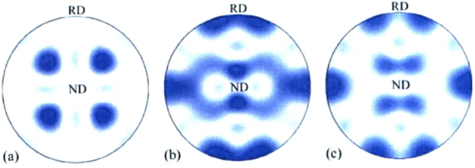
Figure 4: {111) pole figures for (a) a cube texture, (b) a copper texture, and (c) a brass texture. "ND" and "RD" correspond to the "normal direction" and the "rolling direction", respectively, of a sample deformed by rolling.

Schematic {11 l} pole figures for a number of commonly observed textures appear in Figure 4, including the cube, copper and brass textures. These projections are conventionally depicted in the plane parallel to that of a sheet sample, and the "normal direction" to this plane is labeled "ND". The transverse direction of highest symmetry is usually called the "rolling direction" and is labeled "RD", although this notation is used for non-rolled materials as well.

Since the geometry of the sample indicates a suitable set of axes for this projection, any sample symmetry is generally visible in the resulting pole figures; for example, samples with orthorhombic symmetry were used to generate the pole figures of Figure 4, meaning that a statistically identical pole figure could be reproduced from any one of the four quadrants. Although this symmetry is occasionally exploited and only a portion of the pole figure provided, it is quite common to find the entire pole figure in the literature.

The same is not true for so-called inverse pole figures. Whereas a pole figure shows sample directions aligned with a particular crystallographic pole, an inverse pole figure does the opposite, indicating the crystallographic poles aligned with a specified sample direction. This is often of interest for samples in which the processing history strongly identifies a single direction, e.g., the axis of a fiber or wire, or the growth direction of a thin film. The procedure for constructing an inverse pole figure is quite similar to that of a pole figure, with one exception; instead of projecting a crystallographic pole onto a plane determined by the sample geometry, the vector pointing along a given sample direction is projected onto planes determined by the local

(19)

crystallographic orientation. That is, the projection procedure illustrated in Figure 3 is performed for each crystal or volume element, with the frame of reference always given by the local crystallographic frame. An inverse pole figure is obtained by plotting the results of all of these projections together.

Figure 5 shows the normal-direction inverse pole figures for samples with the three textures shown in Figure 4, namely, the cube, copper and brass textures. Since the frame of reference for an inverse pole figure is always defined by the local crystal orientation, the symmetry of the crystals is reflected in the inverse pole figures. As indicated by the fine lines in Figures 5a, 5c and 5e, the cubic crystal symmetry of the samples with these textures divides the projections into twenty-four stereographic triangles, each containing identical orientation information. The crystal symmetry is exact, rather than statistical as is the case for sample symmetry, allowing the entire inverse pole figure to be recovered exactly from any one of the stereographic triangles. Hence, the twenty-four-fold redundancy strongly encourages presentation by a single stereographic triangle. The standard stereographic triangle of the cubic system is that

010 010 ₀₁₀ : 100 100 00 . .. (a) (C) (e) (b) .(d) _. _(f) _{" -.} 001 101 001 101 001 101

Figure 5: _{Normal-direction inverse pole figures for the three textures in Figure 4. The inverse pole figure at}

the top of a given column is divided into twenty-four stereographic triangles, with the standard stereographic triangle outlined. This triangle appears alone at the bottom of the column. Miller indices in the figure refer to directions in the local crystallographic frame. (a) A cube texture, and (b) the standard stereographic triangle of the cube texture. (c) A copper texture, and (d) the standard stereographic triangle of the copper texture. (e) A brass texture, and (f) the standard stereographic triangle of the brass texture.

(20)

containing the crystallographic directions {hkl} for which 1 > h 2 k 2 0, which we have outlined using bold lines in Figure 5. The usual presentation of an inverse pole figure provides only this standard stereographic triangle, as shown in Figures 5b, 5d and 5f.

It is important to remember that pole figures and inverse pole figures do not explicitly indicate the orientations of crystals in a polycrystalline sample, only the orientations of selected crystalline planes or directions. As suggested by Figure 1, these constructions represent only a fraction of the orientation information that is accessible via techniques that include EBSD. Occasionally, multiple pole figures, each of a different crystallographic axis, may be presented as a means of illustrating texture; however, there is no explicit means to identify the points on two pole figures originating from a single crystal. There do exist highly developed methods for determining the most probable crystal orientation distribution consistent with the pole figures of multiple crystallographic planes [4], but in general pole figures unnecessarily discard a great deal of the available orientation information. Therefore, methods of texture representation that accurately reflect the orientations of the crystals, rather than their planes, are frequently more useful than representation by pole figures.

1.3. Discrete Orientations

Any real, orthogonal, three-by-three matrix of determinant one corresponds to a proper rotation of space in the active convention. The group of rotation matrices with these properties is often considered to be the canonical parameterization of rotations, partly due to the simplicity of applying a rotation matrix to either a vector or to another rotation matrix via the matrix product. As a result, rotation matrices are quite convenient for the algebraic manipulation of discrete orientations; on the other hand, the visualization of a collection of orientations via rotation matrices is rather difficult.

A unique description of an orientation in three dimensions only requires three independent parameters [8]. If these can be identified, they can be taken as coordinates of a three-dimensional group space in which individual orientations appear as points. In the case of rotation matrices, each matrix contains nine components. While the direct use of these nine components to form a nine-dimensional group space is unreasonable, there is no obvious way to use only three of the matrix components to represent an orientation

(21)

(though there is some motivation for using six [9, 10]). A related difficulty lies in interpreting the physical effect of a rotation matrix; at least to the current authors, this is not transparent except in the simplest cases. The regrettable result is that the use of this convenient and familiar parameterization of rotations is sharply restricted to the algebraic manipulation of discrete orientations, rather than to their visualization.

Partly for this reason, the materials science community employs a number of other parameterizations side by side with rotation matrices, each with their own particular advantages and weaknesses. The analysis of texture information requires familiarity with the most common parameterizations in order to be able to select the most appropriate one for the application at hand. We provide a brief overview of these parameterizations in this section, with particular emphasis on their relative strengths.

1.3.1. Axis-Angle Parameters

A theorem due to Euler states that every displacement of a sphere with a fixed center is equivalent to some rotation of that sphere about an axis by an angle [11]. Although this description of a rotation requires four parameters, three for the coordinates of the unit vector n pointing along the axis of rotation and one for the angle co, it has the advantage that the physical effect of a rotation described by an axis and angle is easily visualized (see Figure 6a). These four parameters may be reduced to three without loss of information by observing that the constraint on the length of n allows only two of its three coordinates to be chosen independently. For instance, n may be expressed in terms of the spherical coordinates 0 and 0, at the expense of introducing an asymmetry into the parameters which is inherent to the spherical coordinate system. As pointed out by Frank [12], a more symmetric method for combining these four parameters into three is to multiply n by a simple function f(c):

s = nf((w). ₍₅₎

Varying the function f(w) converts the quantity s into various neo-Eulerian mappings. The close relationship between the axis and angle of a rotation and the corresponding point in the group space of one of these neo-Eulerian mappings is illustrated in Figure 6.

(22)

(a) Jx ₍_(b)Is,

-Figure 6: Relationship of the vector n and angle w to the parameters of a neo-Eulerian mapping. (a) The result of any series of rotations is equivalent to some rotation, performed about an axis parallel to

n by an angle co. The vector n can be written in terms of the spherical angles 0 and 0. (b) The

corresponding point in the group space of a neo-Eulerian mapping with parameters s = nf(co). The result is nearly as straightforward to interpret as the description using n and w directly. The simplest function of this type is the rotation angle itself. The vector a then points in the same direction as the axis of rotation and scales linearly in length with the rotation angle:

a = nco. (6)

We refer to the components of a, and not the four parameters of the separate axis and angle of rotation, as the axis-angle parameters because their behaviour is more reasonable for small rotations and because they appear more often in the literature. Since n may point in any direction and co is constrained to the values 0 co _; z, the group space of

these parameters is a solid ball of radius ir. Each point on the interior of this ball corresponds to a unique rotation, and diametrically opposed points on the surface correspond to the same two-fold rotation. While the redundant points can be removed by excluding certain portions of the surface [13], the topological properties of the space nevertheless allow small variations in a physical orientation to correspond to discontinuous changes in the axis-angle parameters as a point jumps from one part of the group space to another. This behaviour is rather inconvenient from the standpoint of numerical calculations.

A more serious drawback of the axis-angle parameterization is the complexity of the multiplication law, or the formula required to calculate the single rotation equivalent to two rotations performed in succession. This difficulty may be addressed by more

(23)

deliberate selection of the function multiplying n, which provides neo-Eulerian parameterizations with simpler combination laws and certain other useful properties. As a result, the simplicity of the axis-angle parameterization is useful when introducing certain ideas concerning the rotation group, but this parameterization is rarely used for the representation of texture due to the existence of more attractive alternatives.

1.3.2. Rodrigues Vectors

The Rodrigues vector parameterization is a neo-Eulerian mapping introduced into the discussion of texture by Frank [12]. The three parameters of a Rodrigues vector are constructed by multiplying n by the tangent of half of w:

r = n tan(c/2). ₍₇₎

As with all of the neo-Eulerian parameterizations, this vector points in the same direction as the axis of rotation and increases monotonically in length with the rotation angle co for angles 0 co zr. Hence, the interpretation of a Rodrigues vector, as with the axis-angle parameters, is nearly as simple as that of the axis and angle of a rotation directly. One disadvantage of this parameterization, though, is that the magnitude of a Rodrigues vector diverges as the rotation angle approaches r, meaning that a binary rotation cannot be represented with a Rodrigues vector. Furthermore, the unbounded group space brings into question the feasibility of visualizing a texture as a collection of points distributed throughout an infinite volume.

Nevertheless, certain properties of Rodrigues vectors make this parameterization quite favorable for the presentation of texture information. These may be derived from the multiplication law for rotations expressed as Rodrigues vectors; the result of a rotation rB followed by a rotation rA is determined by [14]

rA +r + rA x rB

rA B ₍₈₎

1- r_A rB

which is a slight rearrangement of the form appearing in the literature. Apart from its relative simplicity, the particular advantage of this multiplication law is that it may be used to show that the trajectory for a continuing rotation about a single axis is a straight

(24)

line in the Rodrigues space, regardless of the orientation of the reference frame; similarly, any change of the reference frame transforms a line into another line, and a plane into another plane [12]. The benefit of these properties becomes apparent when considering the effect of symmetry on the group space.

The presence of sample or crystal symmetry partitions the group space into distinct regions known as fundamental zones, defined by the requirement that they contain a unique point for every physically distinguishable orientation of a crystal. That is, a given fundamental zone contains only one of the points corresponding to the set of symmetrically equivalent rotations SOCj. The presence of symmetry thereby reduces the matter of visualizing the group space to that of a single fundamental zone, since all of the texture information is contained in each fundamental zone. While for most parameterizations the surfaces of these fundamental zones are curved, it follows from Equation (8) that the boundaries of the fundamental zones in Rodrigues space are always planar [12]. The specific forms of these fundamental zones have been derived for a variety of crystal and sample symmetries, and are generally finite and bounded by planar surfaces [14, 15]. For materials with sufficiently high crystal symmetry, this has encouraged the presentation of texture information in two dimensions by equidistant

? 3 3 ,s t= 0.368 r= 0.276 r,=0.184

r/

S. ~ =0.092 r,=0.000 ,=-0.092

(b) r,= -0.184 r = -0.276 i = -0.368

Figure 7: A collection of discrete orientations from a copper textured material with cubic crystal symmetry, depicted in the fundamental zone of Rodrigues space. (a) The cubic fundamental zone containing the origin is a truncated cube with six octagonal faces and eight triangular faces. (b) The distribution is conventionally plotted in equidistant sections perpendicular to the r3axis.

(25)

planar sections of the fundamental zone. This presentation is used in Figure 7 for a collection of orientations from a copper textured material with cubic crystal symmetry. Figure 7a displays the orientations in the cubic fundamental zone, and Figure 7b gives the conventional sections of this space in two dimensions.

1.3.3. Quaternions

Although quaternions often receive less notice than other parameterizations, their attractive mathematical properties have proven indispensable for a number of subjects with particular relevance to the analysis of orientation information. Specifically, quaternions have been used for texture analysis [12, 16-19], disorientation and mean orientation calculations [5, 15, 20-25], expression of certain specific textures [26-28], and in connection with the equations of texture evolution [29, 30]. Quaternions appear in related fields of materials science as well, as in the development of the theory of coincident site lattices [21, 31, 32] and in the investigation of the symmetry groups for modulated crystals and quasicrystals [33].

A quaternion q is often interpreted as a vector in four-dimensional space. For the study of rotations, the quaternions of interest satisfy the normalization constraint q2 + q + q2 + q3 = 1, which is assumed throughout the remainder of this document. A

quaternion is then related to the quantities n and o of a rotation by

q = (q0,q)= [cos(w/2),n sin(w/2)], ₍₉₎

where qo and q are conventionally referred to as the scalar and vector parts of the quaternion, respectively. While the description of a three-dimensional rotation requires three parameters and a quaternion contains four, we observe that a rotation is completely specified by just the vector part q, which may be interpreted as a neo-Eulerian mapping. Although the scalar part qo appears redundant, the properties of this four-component parameterization strongly encourage the use of the parameter qo as well, at the price of a little redundancy.

As normalized vectors in four-dimensional space, quaternions inhabit the region defined as the set of points at a distance of one from the origin, i.e. the unit sphere in four dimensions (or S3_,_{for those familiar with this notation). Exactly as for a sphere in three}

(26)

dimensions, there is no closed path on the unit sphere in four dimensions that contains a discontinuous change in the values of the quaternion components; the discontinuous change in the values of the axis-angle and Rodrigues vector parameters for rotations in the vicinity of co = ;r is simply not present. By including all of the quaternions on this hypersphere, though, every physical orientation is represented twice. Equation (9) indicates that given a quaternion +q, increasing co by 2;r results in the antipodal quaternion -q with the signs of all the components reversed. Although these quaternions correspond to distinct rotations, they clearly result in the same physical orientation (meaning that one may consider the space inhabited by orientations as RP3). This may be interpreted as resulting from the trivial symmetry of three-dimensional space, that is, a rotation by 2;r about any axis results in an indistinguishable orientation. As in Rodrigues space, the presence of symmetry partitions the quaternion group space into distinct fundamental zones (actually, Heinz and Neumann derived the boundaries of these regions in Rodrigues space from the properties of the quaternion group space [15]). The symmetry through a rotation by 2;" identifies the fundamental zones as one half of the unit sphere, and we select the half with positive values of qo for the representation of textures. Hence, the parameterization of a single orientation by two quaternions is not a particularly serious obstacle.

The advantage of writing the quaternion in Equation (9) in terms of half-angle trigonometric functions (and thereby introducing the redundancy in +q and -q) rather than full-angle functions is that this form permits the multiplication law to be written in

an exceptionally simple form; a rotation expressed by the quaternion q followed by qA results in the quaternion given by [13]

[qqAo9A ,qB ]= [qAoqBo- 9qA q9B'qAOqB + q ₀q9A +9A xqB], (10)

where quaternions operate to the right. The simplicity of this multiplication law lies in the fact that the components of the resulting quaternion are all linear functions of the components of q, and q. Although this is a feature of other parameterizations as well (e.g. rotation matrices), the quatemion parameterization is the parameterization of smallest dimension with this property [10]. With respect to numerical calculations, this

(27)

type of multiplication law tends to be efficient and robust, and there is some indication that quaternions may even be preferable to rotation matrices for this purpose [34].

There remains the matter of visualizing a collection of points embedded in a four-dimensional space, i.e., of the necessity of projecting from four dimensions to three, and from three dimensions to two. While there are many projections of the quaternion group space with qo 2 0 into three dimensions, we mention only the orthographic and gnomic projections at the moment (stereographic and equal-volume projections into three dimensions should generally be considered as well, though the formulas for these are slightly more complex [6, 12]). The first, the orthographic projection, follows from the observation that the vector part q of a quaternion q resembles a neo-Eulerian mapping, for which all orientations may be plotted in the analog of the representative spherical volume in Figure 6b. _{This method is attractive because there is little additional} computation involved, and knowledge of the vector part allows the final component of the quaternion to be quickly reconstructed by applying the normalization constraint. An

0 ₀

00 to 150 150 to 300 300 to 450 450 to 600 600 to 750 _{75 to 900} _{900 to 1050} 105" to 120' 1200 to 1350 1350 to 1500 (a) q1 _{/__} (b) 1500 to 1650 1650 to 1800

Figure 8: A collection of discrete orientations from a copper textured material with cubic crystal symmetry,

depicted _{in (a) the three dimensions inhabited by the vector part q of a quatemion q, and (b) in two}

dimensions as a _{collection of stereographic projections of concentric spherical shells of the space}

in (a). This presentation is naturally suited to the spherical shape of the space, and has the advantage that the rotation angle is constant within a given spherical shell, promoting an intuitive interpretation of points displayed in this format.

Analysis of crystallographic texture information by the hyperspherical harmonic expansion

JUL 2 8 2009

LIBRARIES

Table of Contents

List of Figures

(10

(,

/w,

1. State of the Field'

0

0

₀