HAL Id: hal-02996675
https://hal.archives-ouvertes.fr/hal-02996675
Submitted on 9 Nov 2020
HAL is a multi-disciplinary open access
archive for the deposit and dissemination of
sci-entific research documents, whether they are
pub-lished or not. The documents may come from
teaching and research institutions in France or
abroad, or from public or private research centers.
L’archive ouverte pluridisciplinaire HAL, est
destinée au dépôt et à la diffusion de documents
scientifiques de niveau recherche, publiés ou non,
émanant des établissements d’enseignement et de
recherche français ou étrangers, des laboratoires
publics ou privés.
The MUSE Hubble Ultra Deep Field Survey. XIII.
Spatially resolved spectral properties of Lyman α haloes
around star-forming galaxies at z > 3
Floriane Leclercq, Roland Bacon, Anne Verhamme, Thibault Garel, Jérémy
Blaizot, Jarle Brinchmann, Sebastiano Cantalupo, Adélaïde Claeyssens, Simon
Conseil, Thierry Contini, et al.
To cite this version:
Floriane Leclercq, Roland Bacon, Anne Verhamme, Thibault Garel, Jérémy Blaizot, et al.. The MUSE
Hubble Ultra Deep Field Survey. XIII. Spatially resolved spectral properties of Lyman α haloes around
star-forming galaxies at z > 3. Astronomy and Astrophysics - A&A, EDP Sciences, 2020, 635, pp.A82.
�10.1051/0004-6361/201937339�. �hal-02996675�
https://doi.org/10.1051/0004-6361/201937339 c ESO 2020
Astronomy
&
Astrophysics
The MUSE Hubble Ultra Deep Field Survey
XIII. Spatially resolved spectral properties of Lyman
α
haloes around
star-forming galaxies at z
>
3
Floriane Leclercq
1,2, Roland Bacon
1, Anne Verhamme
2, Thibault Garel
1,2, Jérémy Blaizot
2, Jarle Brinchmann
3,4,
Sebastiano Cantalupo
5, Adélaïde Claeyssens
1, Simon Conseil
1, Thierry Contini
6, Takuya Hashimoto
7,
Edmund Christian Herenz
8, Haruka Kusakabe
2, Raffaella Anna Marino
5, Michael Maseda
4, Jorryt Matthee
5,
Peter Mitchell
4, Gabriele Pezzulli
5, Johan Richard
1, Kasper Borello Schmidt
9, and Lutz Wisotzki
91 Univ Lyon, Univ Lyon1, Ens de Lyon, CNRS, Centre de Recherche Astrophysique de Lyon UMR5574, 69230 Saint-Genis-Laval,
France
2 Observatoire de Genève, Universite de Genève, 51 Ch. des Maillettes, 1290 Versoix, Switzerland
e-mail: [email protected]
3 Instituto de Astrofísica e Ciências do Espaço, Universidade do Porto, CAUP, Rua das Estrelas, 4150-762 Porto, Portugal 4 Leiden Observatory, Leiden University, PO Box 9513, 2300 RA Leiden, The Netherlands
5 Department of Physics, ETH Zürich, Wolfgang-Pauli-Strasse 27, 8093 Zürich, Switzerland
6 Institut de Recherche en Astrophysique et Planétologie (IRAP), Université de Toulouse, CNRS, UPS, 31400 Toulouse, France 7 Tomonaga Center for the History of the Universe (TCHoU), Faculty of Pure and Applied Sciences, University of Tsukuba, Tsukuba,
Ibaraki 305-8571, Japan
8 ESO Vitacura, Alonso de Córdova 3107, Vitacura, Casilla 19001, Santiago de Chile, Chile 9 Leibniz-Institut fur Astrophysik Potsdam (AIP), An der Sternwarte 16, 14482 Potsdam, Germany
Received 17 December 2019/ Accepted 6 February 2020
ABSTRACT
We present spatially resolved maps of six individually-detected Lyman α haloes (LAHs) as well as a first statistical analysis of the Lyman α (Lyα) spectral signature in the circum-galactic medium of high-redshift star-forming galaxies (−17.5 > MUV > −21.5)
using the Multi-Unit Spectroscopic Explorer. Our resolved spectroscopic analysis of the LAHs reveals significant intrahalo variations of the Lyα line profile. Using a three-dimensional two-component model for the Lyα emission, we measured the full width at half maximum (FWHM), the peak velocity shift, and the asymmetry of the Lyα line in the core and in the halo of 19 galaxies. We find that the Lyα line shape is statistically different in the halo compared to the core (in terms of width, peak wavelength, and asymmetry) for ≈40% of our galaxies. Similarly to object-by-object based studies and a recent resolved study using lensing, we find a correlation between the peak velocity shift and the width of the Lyα line both at the interstellar and circum-galactic scales. This trend has been predicted by radiative transfer simulations of galactic winds as a result of resonant scattering in outflows. While there is a lack of correlation between the spectral properties and the spatial scale lengths of our LAHs, we find a correlation between the width of the line in the LAH and the halo flux fraction. Interestingly, UV bright galaxies (MUV < −20) show broader, more redshifted, and less
asymmetric Lyα lines in their haloes. The most significant correlation found is for the FWHM of the line and the UV continuum slope of the galaxy, suggesting that the redder galaxies have broader Lyα lines. The generally broad and red line shapes found in the halo component suggest that the Lyα haloes are powered either by scattering processes through an outflowing medium, fluorescent emission from outflowing cold clumps of gas, or a mix of both. Considering the large diversity of the Lyα line profiles observed in our sample and the lack of strong correlation, the interpretation of our results is still broadly open and underlines the need for realistic spatially resolved models of the LAHs.
Key words. galaxies: high-redshift – galaxies: formation – galaxies: evolution – cosmology: observations 1. Introduction
Lyman α λ1215.67 (Lyα) emission is the brightest recombina-tion line of the hydrogen atom. As such, a number of galaxies at various redshifts have been discovered through the detection of the Lyα line (e.g., Cowie & Hu 1998; Malhotra & Rhoads 2002;Ouchi et al. 2003,2008,2010). Lyα emission has there-fore become a prime tool for the exploration of the Universe and, particularly, in the study of the distant and faintest star-forming galaxies which represent the bulk of the galaxy population in the early Universe.
While historically it was seen simply as a powerful tool for detecting high redshift objects, it is now possible to use Lyα
emission as a tracer of the interstellar medium (ISM) of galaxies as well as their gaseous envelopes, known as the circum-galactic medium (CGM). It also traces the gas exchanges between a galaxy and the environment which primarily drives its evolution. The cold circum-galactic gas is observed in emission in the form of a Lyα halo (LAH) which reflects the properties of the medium in terms of H
i
gas kinematics, column density, and opacity.Detecting diffuse LAHs around high-redshift star-forming galaxies is very challenging because of sensitivity limitations. The first tentative detections of extended Lyα emission using narrowband (NB) imaging were reported twenty years ago by Møller & Warren (1998). In order to counteract those limitations, a number of authors adopted stacking methods
(e.g., Fynbo et al. 2001;Hayashino et al. 2004;Matsuda et al. 2012;Momose et al. 2014;Xue et al. 2017) and provided statis-tical evidence for the ubiquity of extended Lyα emission around classical Lyα emitters (LAE). Yet these statistical methods have been criticized and contradictory results reported (e.g., Bond et al. 2010; Feldmeier et al. 2013) casting doubts on the exis-tence of the LAHs. While extended Lyα emission has then been observed around individual massive galaxies and quasars (e.g.,
Steidel et al. 2000,2011; Matsuda et al. 2004,2011; Miley & De Breuck 2008;Cantalupo et al. 2012), the detection of LAHs around low-mass star-forming galaxies was difficult and required expensive procedure, such as the acquisition of an ultra-deep long-slit observation (Rauch et al. 2008) or the use of the mag-nification power of gravitational lensing (Swinbank et al. 2007). When it was installed at the Very Large Telescope (VLT/ ESO) three years ago, the Multi-Unit Spectroscopic Explorer (MUSE, Bacon et al. 2010), thanks to its unrivaled sensitivity, revolutionized the study of the cold CGM of star-forming galax-ies by allowing the detection of LAHs around 21 individual low-mass and distant galaxies (Wisotzki et al. 2016; hereafter W16) in the MUSE Hubble Deep Field South (Bacon et al. 2015). One year later, we (Leclercq et al. 2017; hereafter L17) extended the W16 LAE sample by a factor of ten using the MUSE Hubble Ultra Deep Field (UDF,Bacon et al. 2017) and reported the detec-tion of LAHs around 80% of our tested sample of LAEs. This result showed the ubiquity of the Lyα haloes around star-forming galaxies at redshift 3 < z < 6, suggesting that there are significant hydrogen reservoirs in their CGM. In the L17 study, we under-took a statistical study of the spatial properties of the detected LAHs. We found that the Lyα emission has a median exponen-tial scale length of 4.5 physical kpc and is, on average, ten times more extended than the UV continuum of the host galaxy. We also performed a detailed investigation of the origin of the LAHs and concluded that we were not able to disentangle the possible mech-anisms: scattering from star-forming regions, fluorescence, cool-ing radiation from cold gas accretion, and emission from satellite galaxies (Gould & Weinberg 1996;Katz et al. 1996;Haiman et al. 2000;Haiman & Rees 2001;Cantalupo et al. 2005;Dijkstra et al. 2006;Kollmeier et al. 2010;Barnes & Haehnelt 2010;Lake et al. 2015).
Another way to get information about the CGM of distant galaxies is to study the spectral properties of the diffuse Lyα emission. Following the pioneering work of Swinbank et al.
(2007) and using the MUSE instrument coupled to the mag-nification power of lensing, such investigations have recently been carried out for a few z > 3 galaxies (Smit et al. 2017;
Vanzella et al. 2017). Those highly magnified systems allow a well-resolved analysis of the Lyα spectral properties. Unfortu-nately, such systems are very rare at high redshift and rely on lens modeling. Until today and aside from very extended Lyα blobs (e.g.,Vanzella et al. 2017), significant spatial variations in the Lyα line profiles have been reported within only three lensed LAHs at z > 3.5 (Patrício et al. 2016;Smit et al. 2017;Claeyssens et al. 2019; hereafter C19) and one un-lensed extended LAE at z '2 (Erb et al. 2018). The resolved study ofErb et al.(2018) reports the detection of spatial variation in the peak ratio and peak separation of a double-peaked Lyα emitter. While the red peak is dominant at the center of the galaxy, the peak ratio becomes close to unity at the outskirts of the halo. The authors indicated that such observations agree with the presence of outflows in the system. They also measured variations of ≈300 km s−1in the Lyα peak separation which they interpreted as variations in the medium properties in terms of column density, covering fraction or velocity. The C19 analysis presents detailed maps of Lyα line
properties (velocity peak shift and width) at sub-kpc scales for two lensed LAEs. For the two objects, significant spatial varia-tions in the line shape were found, as well as a global trend for the Lyα line to be redder and wider at large radii.
Following those recent studies, here we go further into the analysis of the diffuse Lyα emission surrounding non-lensed galaxies by looking at the spatially resolved properties of the Lyα haloes detected in our previous study L17. A significant improvement in the data reduction of the MUSE UDF data (Bacon et al., in prep.) allows for a detailed analysis of the brightest LAHs. By taking advantage of the three-dimensional (3D) information provided by the MUSE data cubes, we first look at spectral variations by creating spatially resolved maps of the Lyα surface brightness and line properties. Then, we adopt an approach similar to L17 and describe the Lyα distribution with two components, but which now also consider the spectral dimension. This 3D parametric method allows us to disentangle the contribution of the central and diffuse components to the total Lyα spectral signature. The connection between the spectral and spatial properties of the LAHs can shed light on their origin, as well as, provide important information about the gas properties in the CGM of the fainter and smaller galaxies, which represent the bulk of the galaxy population at high redshift.
The paper is organized as follows: we describe our data and sample construction in Sect.2. Section3explains our binning and fitting procedures for the construction of spatially resolved maps of the Lyα distribution. Section4describes the model that we use to determine the spectral characteristics of the LAHs presented in Sect.5. Section5also includes a statistical comparison with the central Lyα line properties. In Sect.6we connect the spectral and spatial Lyα properties and investigate the link with the UV properties of the host galaxies. Finally, we discuss and present our summary and conclusions in Sects.7and8, respectively.
In this paper, we use AB magnitudes, physical distances and assume aΛCDM cosmology with Ωm= 0.3, ΩΛ= 0.7 and
H0= 70 km s−1Mpc−1.
2. Data and sample definition 2.1. Observations and data reduction
The MUSE UDF data were taken as part of the MUSE Guaran-tee Time Observations program between September 2014 and February 2016 under a clear sky, photometric conditions and good seeing (full width at half maximum, FWHM, of 000. 6 at
7750 Å). More details about the data acquisition can be found inBacon et al.(2017).
Several 10×10pointings (corresponding to the MUSE field of
view) were completed at two levels of depth: a 30× 30
medium-deep field consisting of a mosaic of nine ten-hour pointings denoted udf-0[1-9] and an ultra-deep field, denoted udf-10, of a single ≈20 h pointing that overlaps with the mosaic reaching a total of ≈30 h depth.
The data reduction of both the udf-10 and mosaic data cubes has been improved with respect to the one we used in L17 (ver-sion 0.41) resulting in less systematics and an improved sky sub-traction. Those latest data cubes (version 1.0) will be described in a forthcoming paper Bacon et al. (in prep.).
The data cubes contain 323 × 322 and 945 × 947 spatial pixels (spaxel) for the udf-10 and mosaic field, respectively. The spatial sampling is 000. 2 × 000. 2 and the spectral sampling
is 1.25 Å. The number of spectra matches the number of spa-tial pixels in each data cube with a wavelength range of 4750 Å to 9350 Å (3681 spectral pixels) and a wavelength-dependent
spectral resolution ranging from ≈180 to ≈90 km s−1 from blue to red (see Fig. 15 of Bacon et al. 2017). The data cubes also contain the estimated variance for each pixel. The data reaches a limiting surface brightness (SB) sensitivity (1σ) of 2.8 and 5.5 × 10⁻²⁰erg s−1cm−2Å−1arcsec−2for an aperture of 100× 100
in the 7000−8500 Å range for the udf-10 and mosaic data cubes, respectively (see Bacon et al., in prep. for more details).
Based on the reduced data cubes presented inBacon et al.
(2017),Inami et al.(2017; hereafter I17) constructed the MUSE UDF catalog. The source detection and extraction were per-formed using (i) priors detected in the Hubble Space Telescope (HST) data (Rafelski et al. 2015), imposing a magnitude cut at 27 in the F775W band for the mosaic field only, and (ii) the ORIGIN detection software (Mary et al. 2020). A complete description of the strategy used for the catalog construction can be found in I17. The ORIGIN software (see Bacon et al. 2017 for techni-cal details) is designed to detect emission lines in 3D data sets. This software enabled the discovery of a large number of LAEs that were barely seen or even undetectable in the HST images (Maseda et al. 2018).
2.2. Lyman alpha emitter sample
Our parent sample was constructed from the MUSE UDF LAH catalog (L17, Sect. 2.2). In this study, extended Lyα emission has been reported around 145 star-forming galaxies between the red-shift range of 3 to 6. From this sample of 145 LAEs, we removed 16 galaxies (i.e., 11%) which have a double-peaked Lyα line pro-file. The study of such objects, which do not represent the bulk of the LAE population, is beyond the scope of this paper and will be subject of a future study. Next, we impose a signal-to-noise ratio (S/N) cut requiring a minimum value of 6 in the core component and in the halo component. The S/N of each compo-nent was calculated in L17 and can be found in Table1. Below this S/N value the 1σ errors on the resulting parameters of our fitting procedure (see Sect.4.1) are very large, on the order of 100 km s−1and 250 km s−1on average for the peak position and width of the line, respectively. Our final sample consists of 19 LAEs surrounded by a Lyα halo: 4 are in the udf-10 field and 15 are found only in the mosaic field.
In this analysis, we use two samples with different S/N cuts: S/N > 6 and S/N > 10. The high S/N subsample consists of six LAEs and is used for our spatially resolved analysis (see Sect.3). The redshift, absolute UV magnitude, Lyα luminosity, Lyα rest-frame equivalent width, and Lyα halo scale length dis-tributions of the parent sample (grey), the S /N > 6 (purple) and the S /N > 10 (red) samples are shown in Fig.1. Those general properties are taken from the Table B.1 of L17 and are summa-rized in Table 1. The UV continuum slopes of our LAEs cal-culated inHashimoto et al. (2017; hereafter H17) and the S/N values of the core and halo component calculated in L17 used for our sample selection are also indicated in this table. In order to test the null hypothesis that our subsamples of LAHs are sim-ilar to the parent sample, we perform a Kolmogorov-Smirnov (KS) test. Our S /N > 6 sample has similar properties to that of the parent sample in terms of redshift (2.99 < z < 5.98) and equivalent width (31.2 < EW0[Å] < 322.5) with KS statistic
DKS < 0.2 and corresponding p-value p0 > 0.5. They are also
statistically similar regarding their halo scale length distributions (2.1 < rshalo[kpc] < 16.4, DKS= 0.33 and p0= 0.05). By
con-struction, our S /N > 6 sample is brighter in Lyα emission (1.5 × 1042 < LLyα[erg s−1] < 2.4 × 1043) and UV continuum
(−18 ≥ MUV≥ −21) with DKS > 0.4 and p0< 0.006.
3. Resolved spectroscopy of the Ly
α
haloesIn order to construct detailed and reliable maps of the diffuse Lyα emission properties around galaxies, we need objects with rela-tively bright Lyα haloes. We therefore run our binning and fitting procedures on the six galaxies of the high S/N subsample. In this spectral study of the Lyα haloes, the measured parameters are the peak velocity shift (∆v) relative to the central (r < 000. 4) line, the
FWHM and the asymmetry parameter (aasym) of the Lyα line.
3.1. Data binning
In order to reveal the spatial variations of the Lyα line pro-files within the extended gaseous haloes, we construct two-dimensional (2D) binned resolved maps. This method allows us to increase the S/N in the outermost parts of the LAH where the surface brightness drops significantly.
The 2D binning is performed on the Lyα NB image con-structed from the MUSE data cube using the Voronoi tessellation method introduced inCappellari & Copin(2003). The spectral window of the NB images varies from source to source and is defined to include the total Lyα line within a spatial aperture of radius rCoG determined by using a curve of growth (CoG)
method1. The borders of the line are set when the flux goes below zero. The spectral bandwidth is then widened by few angstroms on each side to ease the fit procedure (see Sect.3.2). This method allows us to encompass all the Lyα flux while limiting the noise. We choose a target S/N of 6 for the binning meaning that the spaxels above this threshold are not combined with others. We note that the S/N values of the bins resulting from the 2D Voronoi binning method (seeCappellari & Copin 2003) are sym-metrically clustered around the target S/N, value of 6 here. This explains why some bins have a S/N lower than 6.
3.2. Line extraction and measurements
We extract the Lyα line in each resulting Voronoi bin and mea-sure its properties by fitting an asymmetric Gaussian function. The line model used was introduced by Shibuya et al. (2014) and is expressed by:
f(λ)= A exp −(λ − λ0)
2
2 (aasym(λ − λ0)+ d)2
!
, (1)
where A, λ0, aasymand d are the amplitude, the peak wavelength,
the asymmetry parameter and a typical width of the line, respec-tively.Shibuya et al.(2014) argue that Eq. (1) provides a more robust peak position for the typical LAE profiles than a sym-metric Gaussian profile. From Eq. (1), we derive the analytic expression for the full width at half maximum (not corrected for instrumental effects) of the line as:
FW H M= 2 √ 2 ln 2 d 1 − 2 ln 2 a2 asym · (2)
In each bin, we fit the Lyα line and its associated variance using the Python package EMCEE (Foreman-Mackey et al. 2013) as our Markov chain Monte Carlo (MCMC) sampler to deter-mine the joint likelihood of our parameters in Eq. (1). We use the measured parameters of the Lyα line integrated in an aperture of radius rCoGas priors for the parameter space exploration.
To perform the fit, we use 50 walkers and run the MCMC for 5000 steps for each Voronoi bin discarding the initial 1000 1 The CoG method is applied on the Lyα NB image optimized in S/N
Table 1. Global properties of our LAEs and their Lyα halo (taken from Table B.1 of L17).
ID z −MUV log10LLyα EW0 β rshalo rscore S/Nhalo S/Ncore
[AB] [erg s−1] [Å] [kpc] [kpc] 82 3.6079 19.82 42.75 85.0 −1.7 ± 0.1 7.00 ± 0.58 0.62 ± 0.01 14.4 14.1 149 3.7218 18.95 42.49 87.7 −2.3 ± 0.1 6.16 ± 0.74 0.51 ± 0.02 11.3 45.2 180 3.4607 18.55 42.19 77.0 −1.7 ± 0.1 3.69 ± 0.96 0.65 ± 0.02 7.1 7.7 547 5.9776 19.02 42.77 150.7 −2.2 ± 0.4 6.61 ± 1.23 0.32 ± 0.02 6.8 24.9 1059 3.8063 21.32 43.09 52.8 −1.2 ± 0.0 6.87 ± 0.45 0.47 ± 0.00 18.1 42.0 1113 3.0905 20.67 42.68 31.2 −1.9 ± 0.0 5.22 ± 0.47 0.99 ± 0.01 19.4 17.4 1185 4.4996 21.17 43.38 97.9 −1.9 ± 0.2 5.73 ± 0.21 1.35 ± 0.00 39.2 35.5 1283 4.3648 20.76 42.86 54.2 −1.5 ± 0.1 5.71 ± 0.51 0.52 ± 0.00 15.9 7.3 1711 3.7662 19.25 42.47 71.8 −1.8 ± 0.2 5.90 ± 1.42 0.59 ± 0.02 6.5 14.3 1723 3.6016 19.15 42.67 134.4 −1.6 ± 0.2 5.23 ± 0.93 0.37 ± 0.01 6.0 30.8 1726 3.7075 19.2 42.79 145.9 −2.0 ± 0.2 5.41 ± 0.59 0.25 ± 0.01 12.6 26.2 1761 4.0284 19.34 42.39 60.0 −1.8 ± 0.2 7.71 ± 1.61 0.49 ± 0.00 6.8 6.2 1817 3.4155 18.86 42.55 120.8 −2.0 ± 0.1 4.45 ± 1.30 0.45 ± 0.01 6.1 17.5 1950 4.4718 19.55 42.49 59.3 −1.7 ± 0.1 11.32 ± 3.06 0.55 ± 0.01 7.3 9.1 2365 3.5975 18.18 42.91 – – 4.77 ± 0.81 0.28 ± 0.01 6.7 10.9 6416 4.2311 19.95 42.88 – – 2.14 ± 0.31 0.22 ± 0.00 10.6 8.4 6680 4.5046 18.86 42.7 139.8 −2.3 ± 0.2 16.43 ± 8.78 0.87 ± 0.02 7.0 105.6 7047 4.2291 19.23 42.62 96.2 −2.1 ± 0.3 4.67 ± 0.99 0.51 ± 0.01 7.6 15.3 7159 2.9958 17.63 42.49 322.5 −2.1 ± 0.4 3.80 ± 0.80 0.29 ± 0.02 7.3 15.1
Notes. ID: source identifier in the MUSE UDF catalog by I17. z: redshift in I17. MUV: absolute far-UV magnitude. log10LLyα: logarithm of the
Lyα luminosity in erg s−1. EW
0: total Lyα rest-frame equivalent width in Å. β: UV continuum slope calculated in H17. rshalo: exponential scale
length of the Lyα halo in physical kpc. rscore: exponential scale length of the UV continuum in physical kpc. S /Nhalo: signal-to-noise ratio of the
Lyα halo. S /Ncore: signal-to-noise ratio of the Lyα core (i.e., “continuum-like”) component.
3 4 5 6 z 0 10 20 30 40 number L17 LAHs S/N > 6 S/N > 10 16 18 20 22 MUV [mag] 0 10 20 30 40 41 42 43 log(LLy /erg s 1) 0 10 20 30 40 0 200 400 EW0 [Å] 0 10 20 30 40 50 5 10 15 rshalo [kpc] 0 5 10 15 20
Fig. 1.From left to right: redshift, absolute UV magnitude, Lyα luminosity, Lyα rest-frame equivalent width, and Lyα halo scale length distributions of the parent sample (grey), the S /N > 6 (purple) and the S /N > 10 (red) samples.
steps. We use the median values of the resulting posterior prob-ability distributions for all the model parameters. The errors on the parameters are estimated using the 16th and 84th percentiles. We check the lines and the corresponding fits in each Voronoi bin. A visual inspection per bin shows that below a S/N of 4, the quality of the fit in the bin is poor. It is confirmed when look-ing at the uncertainties of the fit parameters. As a consequence, we reject the bins whose S/N is lower than 4. The selected bins are located in areas where the surface brightness is brighter than 10−18erg s−1cm−2arcsec−2. We also check the reduced χ2 and
found that it is <1.5 and >0.1 for all the S /N > 4 fitted lines and <1 for more than 90% of the spectra for each object. This result confirms that the Lyα lines are fairly well described by an asymmetric Gaussian function.
3.3. Resolved Lyα spectral properties
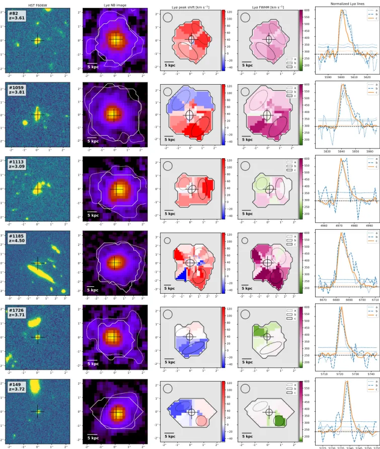
The Lyα emission maps of the six galaxies which meet our S/N criterion are shown in Fig. 2. By requiring a S /N > 4 in the bins (see Sect.3.2), our maps consist of 14, 41, 23, 106, 16 and 21 bins for object #82, #1059, #1113, #1185, #1726 and #149, respectively, probing the LAH in a radius of ≈10−15 kpc. In
order to facilitate the visual comparison between the central and the halo components of the galaxies, the diverging colormaps of the peak velocity shift and FWHM maps (third and fourth columns, respectively) are centered on the best-fit parameter val-ues of the Lyα line extracted in the central region (aperture of radius 0.400 or 2 MUSE pixels) of the galaxy. By construction,
the central best-fit peak value is very close (<25 km s−1 di ffer-ence) to the position corresponding to the Lyα redshift from the I17 catalog where a point spread function (PSF) weighted extraction has been used. The last column in Fig. 2 shows the Lyα lines extracted in three different and arbitrarily chosen regions, one is located in the inner region of the galaxy (solid orange ellipse) and the others in the surrounding halo (dotted and dashed blue ellipses).
It is apparent from Fig. 2that the LAEs exhibit significant differences in their line profiles as a function of spatial position. 3.3.1. Lyα line properties
The resolved maps of the Lyα peak velocity shift (third column) reveal that the peak position does vary. The amplitudes of those variations are lower than ≈200 km s−1for the six tested objects.
-2'' -1'' 0'' 1'' 2'' -2'' -1'' 0'' 1'' 2'' HST F606W #82 z=3.61 -2'' -1'' 0'' 1'' 2'' -2'' -1'' 0'' 1'' 2'' 5 kpc Ly NB image -2'' -1'' 0'' 1'' 2'' -2'' -1'' 0'' 1'' 2'' 5 kpc Ly peak shift [km s1] 40 20 0 20 40 60 80 100 120 -2'' -1'' 0'' 1'' 2'' 5 kpc Ly FWHM [km s1] a b c 200 250 300 350 400 450 500 550 600 5590 5600 5610 5620 Normalized Ly lines a b c -2'' -1'' 0'' 1'' 2'' -2'' -1'' 0'' 1'' 2'' #1059z=3.81 -2'' -1'' 0'' 1'' 2'' -2'' -1'' 0'' 1'' 2'' 5 kpc -2'' -1'' 0'' 1'' 2'' -2'' -1'' 0'' 1'' 2'' 5 kpc 4020 0 20 40 60 80 100 120 -2'' -1'' 0'' 1'' 2'' 5 kpc a b c 200 250 300 350 400 450 500 550 600 5830 5840 5850 5860 a b c -2'' -1'' 0'' 1'' 2'' -2'' -1'' 0'' 1'' 2'' #1113 z=3.09 -2'' -1'' 0'' 1'' 2'' -2'' -1'' 0'' 1'' 2'' 5 kpc -2'' -1'' 0'' 1'' 2'' -2'' -1'' 0'' 1'' 2'' 5 kpc 4020 0 20 40 60 80 100 120 -2'' -1'' 0'' 1'' 2'' 5 kpc a b c 200 250 300 350 400 450 500 550 600 4960 4970 4980 4990 a b c -3'' -2'' -1'' 0'' 1'' 2'' 3'' -3'' -2'' -1'' 0'' 1'' 2'' 3'' #1185 z=4.50 -3'' -2'' -1'' 0'' 1'' 2'' 3'' -3'' -2'' -1'' 0'' 1'' 2'' 3'' 5 kpc -3'' -2'' -1'' 0'' 1'' 2'' 3'' -3'' -2'' -1'' 0'' 1'' 2'' 3'' 5 kpc 40 20 0 20 40 60 80 100 120 -3'' -2'' -1'' 0'' 1'' 2'' 3'' 5 kpc a b c 200 250 300 350 400 450 500 550 600 6670 6680 6690 6700 6710 a b c -2'' -1'' 0'' 1'' 2'' -2'' -1'' 0'' 1'' 2'' #1726 z=3.71 -2'' -1'' 0'' 1'' 2'' -2'' -1'' 0'' 1'' 2'' 5 kpc -2'' -1'' 0'' 1'' 2'' -2'' -1'' 0'' 1'' 2'' 5 kpc 4020 0 20 40 60 80 100 120 -2'' -1'' 0'' 1'' 2'' 5 kpc a b c 200 250 300 350 400 450 500 550 600 5710 5720 5730 5740 a b c -2'' -1'' 0'' 1'' 2'' -2'' -1'' 0'' 1'' 2'' #149 z=3.72 -2'' -1'' 0'' 1'' 2'' -2'' -1'' 0'' 1'' 2'' 5 kpc -2'' -1'' 0'' 1'' 2'' -2'' -1'' 0'' 1'' 2'' 5 kpc 4020 0 20 40 60 80 100 120 -2'' -1'' 0'' 1'' 2'' 5 kpc a b c 200 250 300 350 400 450 500 550 600 5725 5730 5735 5740 5745 5750 5755 a b c
Fig. 2.Sample of six LAEs surrounded by a Lyα halo with S /N > 10 from the L17 sample. Each row shows a different object. First column: HST/F606W image of the LAE. The HST coordinates (Rafelski et al. 2015) are indicated by the black cross in all panels. The MUSE ID and z are indicated. Second column: Lyα narrowband image (plotted with a power-law stretch) with SB contour at 10−18erg s−1cm−2arcsec−2(dashed
white). The solid white contour shows the outer limit of the Voronoi bins group (S /N > 4) used in this study (see Sect.3.1). Third column: map of the Lyα line peak velocity shift relative to the central (r < 000.4) Lyα line peak (see Sect.3.3). The diverging colormaps are centered on the
parameter values of the central line and have the same dynamical range to ease the visual comparison. The FWHM of the PSF is plotted in the upper-left corner. Fourth column: map of the Lyα line FWHM. Fifth column: lines extracted in the ellipsoid areas designated by the same line style on the maps. They aim to highlight the spectral variations in the core and halo components. The dotted and dashed colored horizontal lines show the 1σ error and the dashed black line shows the zero.
300 400 500 FWHM [km s1] 200 100 0 100 200 Ly p ea k s hif t [ km s 1] =0.62 p0=1.7e-02 #82 best fit=0.7±0.2 300 400 500 600 FWHM [km s 1] =0.69 p0=5.1e-07 #1059 best fit =0.36±0.05 300 400 FWHM [km s1] =0.45 p0=3.2e-02 #1113 best fit=0.5±0.1 500 1000 FWHM [km s 1] =0.58 p0=1.1e-10 #1185 best fit =0.31±0.04 200 250 FWHM [km s1] =-0.02 p0=9.4e-01 #1726 best fit=0.1±0.2 175 200 225 250 FWHM [km s 1] =-0.19 p0=4.1e-01 #149 best fit=0.6±0.2 0 50 100 peak shift [km s 1] 1018 1017 SB [e rg s 1 cm 2 ar cs ec 2] #82 0 100 200 peak shift [km s1] #1059 0 50 100 150 peak shift [km s 1] #1113 0 100 200 peak shift [km s1] #1185 50 25 0 25 peak shift [km s 1] #1726 50 0 50 peak shift [km s1] #149 300 400 500 FWHM [km s 1] 1018 1017 SB [e rg s 1 cm 2 ar cs ec 2] 300 400 500 600 FWHM [km s 1] 300FWHM [km s4001] 500FWHM [km s10001] FWHM [km s200 2501] 150 FWHM [km s200 1]250
Fig. 3.Lyα haloes spectral analysis of the six galaxies presented in Fig.2. First row: peak velocity shift relative to the central Lyα line (r < 000.4)
plotted against the FWHM of the Lyα lines extracted in the different Voronoi bins for the six tested objects (MUSE IDs are indicated). The brightness of the points indicates the bin surface brightness (darker point meaning higher SB). Pearson correlation coefficients ρ and corresponding p0values are shown in each panel. The solid colored line indicates the best fit of our data, while the dashed colored lines show the 1σ errors (the
slope α and its error are indicated in the legend). The square point (last panel) is discarded for the fit (sigma clipping factor of 4). The parameters measured on the total Lyα lines are indicated by the star symbols. For comparison the re-scaled V18 relation (solid line) and its dispersion (dotted lines) are plotted in black. The black dashed lines show the V18 relation 1σ errors by taking into account the errors of the re-scaling procedure (see Sect.3.3.2). Bottom rows: Lyα surface brightness of the bins as a function of the peak velocity shift (top) and FWHM (bottom) of the Lyα line for the six tested objects. The black dotted vertical lines indicate the central Lyα line values. The black horizontal dashed line represents the arbitrary SB threshold at 10−17erg s−1cm−2arcsec−2. The colored vertical dashed lines show the median values of the SB < 10−17erg s−1cm−2arcsec−2bins.
We do not observe any obvious velocity field in the Lyα distri-butions except for the object #1059 (second row) and possibly object #1726 (second to last row) where a structured velocity field is suggested (see discussion in Sect.7.2).
The resolved maps of the Lyα FWHM (fourth column) reveal that the width of the Lyα line varies spatially as well. The ampli-tude of those variations can be higher, notably for the objects #1059 and #1185 for which the line width variations reach ≈250 and >500 km s−1, respectively.
Generally, a large diversity in the line profiles is observed: while some galaxies globally show a wider and redder Lyα line in the outer regions (e.g., objects #82, #1059 and #1113), others show slightly narrower and bluer lines (e.g., objects #1726 and #149). One can also observe spectral variations at small spatial scales (<5 kpc) within the LAHs. The last column of Fig.2 illus-trates some of those spectral changes by showing three spectra integrated in three arbitrarily chosen regions. Interestingly, the Lyα line extracted in the bins are all single-peaked except for object #149 where a blue bump is visible (dashed line) although its S/N is low (see discussion Sect.7.3.3).
3.3.2. Peak velocity shift versus width of the Lyα line
The top row of Fig.3displays the relation between the best-fit parameters of the Lyα lines extracted in the different bins for the six tested objects in terms of peak velocity shift and FWHM. The points are color coded by the SB of the bins (darker point meaning higher SB).
We find a significant correlation between the Lyα peak veloc-ity shift and the FWHM for four objects out of six (see the Pearson coefficients). This result is in good agreement with C19 which also found this correlation for spatially resolved spectra of two lensed galaxies. For #1726 and #149, the small dynamic range in FWHM and peak velocity shift precludes any statement about the lack of existence of a correlation with the present data. We compare our results to the empirical relation established inVerhamme et al.(2018; hereafter V18) between the Lyα peak velocity shift relative to the systemic redshift and the FWHM of the Lyα line. This object-by-object based relation has been established using 13 LAEs detected in various MUSE fields for which the systemic redshift is known as well as spectroscopic
Lyα data found in the literature spanning a wide redshift range. We performed a vertical re-scaling of the V18 relation (using a least-squares minimization method) in order to aid the visual comparison of the slopes. This is due to the fact that we do not know the systemic redshift of our objects. The re-scaled V18 relation (solid black line) and its dispersion (dotted black lines) are superimposed on our data in Fig.3(top row). Remarkably, most of our data points fall close to this relation and within its 1σ dispersion. The dashed black lines represent the V18 disper-sion when including the errors from our re-scaling procedure. The colored solid and dashed lines show our best fit to the data and the 1σ errors, respectively. Similarly to V18, we run the LTS_LINEFIT routine2 introduced in Cappellari et al. (2013)
which uses a robust least-squares fitting technique and takes into account the errors of both variables. A sigma-clipping factor of 4 is used in the fit procedure. The excluded point is shown by the square symbol (last panel).
We find a trend similar as V18 for spatially resolved spectra but the slope of the relation is lower and varies from one object to another (see values on Fig.3, top row). Interestingly, the best-fit parameters measured on the total Lyα lines (extracted in an aperture of radius rCoG) of the six objects (black star symbols)
are well located on the V18 relation. 3.3.3. Surface brightness effects
The bottom rows of Fig. 3shows the surface brightness in the bins as a function of the Lyα peak velocity shift relative to the Lyα central line (top panels) and the FWHM of the line in the Voronoi bins (bottom panels). In a similar way to C19, the vertical dashed lines show the median values of the faintest bins (SB < 10−17erg s−1cm−2arcsec−2, horizontal dashed line).
On average, the Lyα lines extracted from the brightest bins (SB > 10−17erg s−1cm−2arcsec−2) have smaller velocity offset (<50 km s−1) and are narrower compared to the ones extracted in
the faintest bins for which we observe more scatter. This result is in good agreement with C19 (see their Fig. 4). We remark that the bins of low SB are also, by construction, the more spa-tially extended and thus more prone to artificial broadening (see Sect.7.2for discussion).
This statement does not apply to object #1726 and #149 for which the variations are smaller. The object #1113 is also inter-esting as we find broad Lyα lines in both faint and bright bins.
All in all, even at the MUSE spectral and spatial resolution, we detect significant variations of the Lyα line profile within the spatial Lyα distribution, for this sample of six bright LAHs with high S/N.
4. Ly
α
halo 3D decompositionIn order to test the robustness of the trends found in the first part of the paper on a larger sample, we set up a new statisti-cal method based on the W16 and L17 analyses which consists of the simultaneous 3D (i.e., spectral and spatial) decomposition of the Lyα emission. This parametric fit procedure is less sensi-tive to the noise. It therefore allows us to increase the sample by including lower S/N Lyα haloes (S/N > 6).
4.1. Three-dimensional two-component fits
Our previous studies (W16 and L17) have demonstrated that the spatial distribution of Lyα radiation emitted from and 2 Cappellari(2014) andhttp://www-astro.physics.ox.ac.uk/
~mxc/software/#lts
around distant star-forming galaxies is well-described by a two-dimensional, two-component circular exponential distribution. In order to push the analysis further, we upgrade the model by adding the spectral dimension to the model. We thus use a 3D, two-component modeling approach, fitting MUSE Lyα subcubes. This method aims to disentangle and compare the averaged Lyα spectral signatures of the host galaxy and its sur-rounding gaseous envelop.
4.1.1. Model
We describe here how we characterize the 3D Lyα distribution of our extended LAEs. In W16 and L17 we decomposed the observed spatial Lyα distribution into a central and an extended circular and co-spatial exponential component using the HST morphological information as prior (see Sect. 4.1 of L17). Using this method, we parametrized the spatial distribution of the Lyα emission with four parameters: the scale lengths and central flux intensities of the central and extended components (rscore, rshalo,
Icore, and Ihalo, respectively). Our 3D model is based on this 2D,
two-component, circularly symmetric model of L17 and addi-tionally takes into account the spectral dimension. It is defined by Eq. (3) where C(r, λ) describes the total Lyα flux distribution in the subcube of the source:
C(r, λ)= " Icore(λ) exp − r rscore ! + Ihalo(λ) exp − r rshalo !# × PSF3D,MUSE(λLyα), (3)
The central flux intensity parameters Icore and Ihalo depend on
the wavelength and are described by the asymmetric Gaussian function given by Eq. (1). Our fit procedure takes into account the MUSE 3D PSF so that the spatial and spectral parameters are corrected from the spatial PSF and line spread function (LSF) effects, respectively.
4.1.2. Subcubes construction
From the MUSE data cubes, we extract subcubes centered on the spectral and spatial flux maxima of our objects. The spatial and spectral apertures used are different for each source. The radius of the spatial aperture corresponds to the measured CoG radius (see Sect. 5.3.2. of L17). The spectral window corresponds to the Lyα full line width extracted in the aperture of radius rCoG
expanded by 2.5 Å (i.e., 2 MUSE pixels) on each side of the line. This 3D aperture ensures that most of the detectable Lyα flux is encompassed for each object while limiting noise. The continuum is removed by performing a spectral median filtering on the MUSE cubes (see Sect. 3.1.1 of L17 for more details).
Following this procedure, we construct Lyα subcubes with spatial and spectral apertures ranging from 100. 8 to 400. 6 (median
value of 200. 8) in radius and 11.25 Å to 31.25 Å (median value of
21.25 Å), respectively. This represents typically a total spectral windows of 1100 km s−1.
4.1.3. Fitting procedure
The modeling is performed by fitting the subcube of our sources by (i) fixing the core and halo scale length parameters rscoreand
rshaloto the values measured in L17 – this step reduces the
num-bers of fitted parameters and therefore makes the fit more robust –, (ii) taking into account the 3D PSF by convolving the model with the MUSE spatial PSF similarly to L17 and the MUSE LSF, and (iii) making use of the variance of each 3D pixel of the subcube.
Table 2. Fitting results from our 3D two-component analysis.
ID FW H MCORE FW H MHALO aasym,CORE aasym,HALO λpeakCORE λpeakHALO ∆vHALO−CORE
[km s−1] [km s−1] [Å] [Å] [km s−1] 82 121+37−28 419+30−29 0.32+0.02−0.03 0.05+0.05−0.05 5599.9+0.2−0.2 5603.7+0.4−0.4 204+32−32 149 55+10−8 37+27−16 0.29+0.01−0.01 0.04+0.17−0.17 5737.9+0.0−0.0 5737.8+0.3−0.3 −4+17−20 180 326+37−41 294+89−110 0.14+0.08−0.08 0.23+0.13−0.17 5421.2+0.6−0.7 5420.3+1.5−0.9 −47+115−88 547 147+22−21 168+105−82 0.37+0.03−0.03 0.19+0.18−0.27 8479.5+0.2−0.2 8480.0+1.0−0.8 17+42−36 1059 224+19−18 420+28−29 0.32+0.02−0.02 0.18+0.06−0.06 5840.5+0.1−0.1 5842.1+0.5−0.5 80+31−31 1113 82+42−26 326+30−31 0.32+0.01−0.01 0.12+0.06−0.06 4970.6+0.2−0.1 4973.1+0.4−0.4 150+35−32 1185 278+14−14 471+15−16 0.30+0.01−0.02 0.12+0.03−0.03 6683.4+0.1−0.1 6685.6+0.3−0.3 99+18−18 1283 192+95−82 458+65−66 0.39+0.05−0.05 0.36+0.09−0.10 6518.5+0.4−0.3 6521.1+0.8−0.7 118+55−48 1711 220+31−39 146+99−114 0.23+0.06−0.06 0.18+0.12−0.20 5792.2+0.4−0.3 5791.5+0.7−0.6 −40+56−50 1723 156+18−16 295+112−98 0.26+0.02−0.02 −0.20+0.34−0.18 5591.8+0.1−0.1 5594.2+1.1−1.5 129+62−84 1726 103+25−25 45+31−16 0.30+0.02−0.02 0.07+0.21−0.18 5720.5+0.1−0.1 5720.8+0.3−0.4 12+20−25 1761 104+101−64 252+207−101 0.38+0.08−0.12 0.21+0.33−0.47 6109.9+0.6−0.6 6111.3+1.7−1.2 67+114−89 1817 135+22−21 33+34−17 0.27+0.02−0.03 0.08+0.13−0.20 5366.0+0.1−0.1 5365.9+0.4−0.3 −2+30−25 1950 240+48−52 285+122−99 −0.15+0.18−0.17 0.14+0.21−0.35 6650.8+0.9−0.9 6648.9+1.9−1.2 −84+123−98 2365 153+38−37 178+80−63 0.32+0.05−0.06 0.25+0.10−0.16 5586.9+0.2−0.2 5588.0+0.6−0.5 64+46−39 6416 294+24−25 115+24−20 0.12+0.04−0.04 0.27+0.03−0.04 6359.1+0.4−0.4 6356.6+0.2−0.2 −115+26−27 6680 106+6−6 70+76−41 0.24+0.01−0.01 0.29+0.07−0.20 6689.3+0.0−0.0 6688.8+0.6−0.6 −22+27−28 7047 143+42−48 141+71−75 0.31+0.04−0.05 0.20+0.11−0.18 6355.0+0.3−0.2 6355.7+0.9−0.5 37+53−36 7159 40+18−18 331+83−85 0.01+0.16−0.14 −0.15+0.11−0.11 4856.4+0.2−0.2 4856.2+0.6−0.7 −12+51−56
Notes. ID: source identifier in the MUSE UDF catalog by I17. FW H MCORE: rest-frame full width at half maximum of the Lyα line extracted in
the core component in km s−1. FW H M
HALO: rest-frame full width at half maximum of the Lyα line extracted in the halo component in km s−1.
aasym,CORE: asymmetry parameter of the Lyα line in the core. aasym,HALO: asymmetry parameter of the Lyα line in the halo. λpeakCORE: peak
wavelength position of the Lyα line in the core in Å. λpeakHALO: peak wavelength position of the Lyα line in the halo in Å.∆vHALO−CORE: halo/core
peak separation in km s−1. Those values are corrected for the MUSE LSF (see TableB.1for non-corrected values). We thus have eight parameters in total to fit the Lyα 3D
dis-tribution: the amplitudes, the peak wavelengths, the asymmetry parameters and the full widths at half maximum of the two asym-metric Gaussian functions describing the flux intensity in the core and halo components as a function of wavelength.
To perform a robust fit of our MUSE subcubes and sim-ilarly to the 1D spectral fit performed in the first part of the paper (see Sect. 3.2), we use the Python package EMCEE (Foreman-Mackey et al. 2013) as our MCMC sampler to deter-mine the joint likelihood of our parameters in Eq. (3). We start by initializing the walkers with the following priors on the parameters:
– The total flux of the lines in the core and halo are equal and are two times smaller than the total Lyα line integrated in an aperture of radius rCoG,
– the wavelength of the core/halo line peaks are equal and correspond to the peak position of the total Lyα line,
– FW H MCORE and FW H MHALO are equal and correspond
to the FWHM of the total Lyα line, – the lines are symmetrical (aasym= 0).
We use 100 walkers and run the MCMC for 5000 steps for each subcubes discarding the initial 1000 steps. We use the median values of the resulting posterior probability distributions for all the model parameters. The errors on the parameters are estimated using the 16th and 84th percentiles. The fitting results are given in Table2.
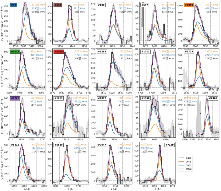
Figure 4 shows the spectral projection of the best-fit 3D model obtained for our 19 LAEs (S /N > 6 sample). We show
the spectral decomposition of the total Lyα line (purple) into the core Lyα line (orange) and the halo Lyα line (blue). We overplot the total observed Lyα line (black line with the 1σ errors shown by the grey area) integrated in the MUSE subcubes (see previous section). For most of our objects, the modeled line is a good fit to the observed Lyα line. The adopted model thus appears to be a good representation of the observed data.
4.2. Model robustness
In order to test our model, we compare the resulting 3D best-fit parameters to the binned resolved Lyα maps (see Fig. 2) obtained in the first part of the paper (Sect. 3). Because the line parameters of the resolved maps are not corrected for instrumental effects, we consider the 3D best-fit parameters not corrected for the LSF (presented in TableB.1) for this exercise.
As a first step, a qualitative visual inspection shows that the trends are similar for the six tested galaxies:
– In Fig.2the objects #82, #1059 and #1185 show broader and redder Lyα lines in the outermost regions of the Lyα spatial distribution. It is in good agreement with the 3D fit parameters.
– On the contrary, the maps of the objects #1726 and #149 indicate that the Lyα lines of the outer bins are bluer and nar-rower compared to the ones of the inner bins, although the vari-ations are small (<30 km s−1). It again agrees with the 3D fit results.
– The resolved maps of the object #1059 are more contrasted in the halo. The shift of the peak goes from ≈−50 km s−1 to
5590 5600 5610 5620 0 50 100 150 200 250 300 350 F [1 0 20 er g s 1 cm 2 Å 1] 121 +3727 km/s 419+2928 km/s 204+3232 km/s #82 5730 5740 5750 0 100 200 300 400 500 5437+98+2615 km/s km/s -4+1719 km/s #149 5410 5420 5430 5440 0 25 50 75 100 125 150 175 325+3741 km/s 293+88109 km/s -46+11587 km/s #180 8470 8480 8490 8500 0 25 50 75 100 125 150 147+2221 km/s 168+10482 km/s 17+4235 km/s #547 5830 5840 5850 5860 0 200 400 600 800 1000 223+1817 km/s 420+2829 km/s 79+3031 km/s #1059 4960 4970 4980 4990 0 200 400 600 800 F [1 0 20 er g s 1 cm 2 Å 1] 82 +4226 km/s 325+3030 km/s 149+3432 km/s #1113 6670 6680 6690 6700 6710 0 200 400 600 800 1000 1200 278+1313 km/s 470+1515 km/s 99+1817 km/s #1185 6510 6520 6530 6540 0 50 100 150 200 250 300 350 400 191+9482 km/s 457+6565 km/s 117+5547 km/s #1283 5780 5790 5800 5810 0 50 100 150 200 250 300 350 220+3138 km/s 145+99113 km/s -39+5549 km/s #1711 5580 5590 5600 5610 0 100 200 300 400 500 600 155+1815 km/s 295+11297 km/s 128+6184 km/s #1723 5710 5720 5730 5740 0 200 400 600 800 F [1 0 20 er g s 1 cm 2 Å 1] 102 +2524 km/s 45+3016 km/s 11+2024 km/s #1726 6100 6110 6120 0 50 100 150 200 103+10063 km/s 251+207100 km/s 67+11488 km/s #1761 5360 5370 5380 0 100 200 300 400 500 600 135+2221 km/s 33+3316 km/s -2+3024 km/s #1817 6640 6650 6660 0 25 50 75 100 125 150 175 239+4751 km/s 284+12299 km/s -84+12397 km/s #1950 5560 5570 5580 5590 5600 0 50 100 150 200 250 300 350 152+3836 km/s 178+7962 km/s 64+4638 km/s #2365 6350 6360 6370 6380 [Å] 0 100 200 300 400 500 F [1 0 20 er g s 1 cm 2 Å 1] 293 +2425 km/s 114+2320 km/s -114+2627 km/s #6416 6680 6690 6700 [Å] 0 100 200 300 400 500 105+56 km/s 69+7641 km/s -21+2727 km/s #6680 6350 6360 6370 [Å] 0 100 200 300 400 143141+41+704774 km/s km/s 36+5235 km/s #7047 4840 4850 4860 4870 [Å] 0 100 200 300 400 500 600 700 40+1818 km/s 330+8284 km/s -11+5055 km/s #7159 data core halo total
Fig. 4.1D profiles of the 3D modeled Lyα distribution decomposed into central (orange lines) and extended (blue lines) components (see Sect.4.1
and Eq. (3)). These represent the 19 galaxies for which the S/N in the core and halo components is higher than 6. The MUSE identifier are indicated
in each panel. The colored labels correspond to the S /N > 10 objects where the same color coding as in Fig.3is used. The total spectra of the modeled Lyα emission are shown in purple. For comparison, the observed Lyα lines and their 1σ errors (see Sect.4.1.2) are overplotted in black and grey respectively. The vertical dotted black lines delimit the spectral window used for the fit (see Sect.4.1.2). The best-fit line parameters (halo/core FWHM and peak separation) are indicated in km s−1(blue, orange and black, respectively) in each panel.
≈+150 km s−1 and the FWHM varies significantly throughout
the halo. In this case the 3D fit provides information about the average Lyα line and as a consequence conceals the spectral variations (see the discussion Sect.7.2). Considering this effect, the line parameters resulting from the two methods are in rather good agreement.
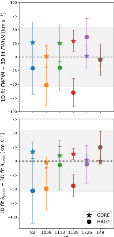
Figure5provides a comparison between the parameter val-ues resulting from the 3D fit procedure and direct measurements using 1D fit. To do so, we extract a core-like (circular aperture of radius <000. 4) and halo-like (annular aperture of radius >100) line
from the subcubes of the six S /N > 10 LAHs and fit those lines with an asymmetric Gaussian function (see Sect.3.2). The peak velocity shift and FWHM values of the two methods are iden-tical within the errorbars and the differences are smaller than one MUSE pixel error (grey shaded area where the error value in km s−1 is set at z= 3) for most of the galaxies. The largest
differences are observed for the objects #1059 and #1185 and are discussed in Sect.7.2). We also note that the central flux of
the halo component is not taken into account for the 1D halo line measurements. This could be responsible for the resulting differences between the two methods.
We underline here that we do not expect the agreement to be perfect, considering that a simple parametric model cannot capture the complex structure and kinematics of the CGM in its entirety, but the fact that we find very good agreement in most cases is reassuring and means that deviations due to additional complexity are not dramatic and that our simple modeling does capture the overall properties of the haloes.
5. Spectral characterization of the Ly
α
emission5.1. Line parameters
The adopted model provides parameters reflecting the width, the peak wavelength and the asymmetry of the Lyα lines cor-rected for LSF for the two components. The top row of Fig.6
100 75 50 25 0 25 50 75 100
1D
fi
t F
W
HM
3
D
fit
FW
HM
[k
m
s
1]
82 1059 1113 1185 1726 149ID
100 75 50 25 0 25 50 751D
fi
t
pe ak3
D
fit
pe ak[k
m
s
1]
CORE HALO CORE HALOFig. 5.Comparison between the core (stars) and halo (dots) line param-eters (top: FWHM, bottom: peak position) resulting from our 3D fit method and 1D fit performed on the Lyα lines extracted in the central region (r < 000.4) and outer regions (r > 100
) of the LAH. This exercise is performed for the six brightest LAHs of our sample (same color coding as Fig.3). The grey shaded area indicates a difference of less than one
MUSE pixel (set for z= 3).
shows the distributions of the core (orange) and halo (blue) line FWHM (left), their peak velocity shift (middle) relative to the peak position of the total fitted line (purple line in Fig. 4) and their asymmetry parameters (right). The median values are indi-cated by the vertical solid lines.
The FWHM values of the Lyα lines span a range from 40 to 325 km s−1 (median value of 147 km s−1) in the core com-ponent and from 33 to 471 km s−1 in the halo (median value of 252 km s−1). The velocity shift∆v values between the peak
of the Lyα line in a given component and the peak of the total Lyα line range from −142 to+75 km s−1in the core and −53 to
+93 km s−1in the halo with a respective median value of −36 and
−6 km s−1. The median asymmetry parameter values are 0.30
and 0.18 and vary from −0.15 to 0.39 and from −0.20 to 0.36 for the core and halo Lyα lines, respectively.
5.2. Halo-Core line profiles comparison
Focusing on the median values of the line parameters in the core and halo taken separately (solid vertical lines in the top panels of Fig.6), the median Lyα line in the halo appears broader, redder, and less asymmetric than the median Lyα line in the core but still asymmetric with a red tail. It is, however, important to note that those distributions show large dispersions (see Sect.5.1).
Now, when comparing the median Lyα line parameters between the components of each galaxy (bottom panels), we see that those differences are less obvious. Indeed, the Lyα line in the halo appears only slightly broader (median value of the FWHM ratio of 1.16, bottom left) and slightly redder (+17 km s−1,
bot-tom middle) than in the core component. On the contrary, the direct core/halo comparison, with a median asymmetry param-eter ratio of 0.5 (bottom right), reinforces the fact that the line in the halo is less asymmetric. It is again important to note here that the dispersion of the distributions is high. The Lyα line in the halo of our galaxies can be up to about two times broader but also narrower than in the core. Some objects have a blueshifted (up to ≈100 km s−1) or redshifted (up to 200 km s−1) Lyα line in the halo compared to the line in the core. We also find that the Lyα line can be more asymmetric in the halo or even show an opposite asymmetry profile (ratio < 0) compared to the line in the core.
Those results demonstrate that the Lyα lines in the halo and in the core can have very different spectral profiles in terms of width, wavelength peak position and asymmetry.
5.3. Halo-Core parameters correlation analysis
We show the most significant correlations between the line parameters in Fig. 7. The relations between all best-fit param-eters are displayed in Fig.A.1.
The results of the Spearman rank correlation test (ρs= 0.56,
p0 = 0.01, left panel) suggest that a positive correlation exists
between the width and the peak velocity shift of the Lyα line in the halo: the wider the Lyα line in the halo is the more it is redshifted compared to the Lyα line in the core. This result is in good agreement with our spatially resolved analysis of the Lyα haloes (Sect.3.3).
We also find that the peak velocity shift of the Lyα line in the halo relative to the peak position in the core correlates with the asymmetry parameter of the central Lyα line (ρs = 0.76,
p0 ' 10−4, right panel). In other words, the more asymmetric
the Lyα line in the core is, the more redshifted the Lyα line in the halo is. This correlation is not seen in the halo component.
We do not find any other significant correlation between the line parameters (see Fig.A.1).
5.4. Statistical significance of the spectral differences In order to answer the question of whether the Lyα line is sig-nificantly different in the central region and in the CGM of our galaxies, we calculate the probability p0of the two line
parame-ter sets (FWHM, λ0, and aasymof the core and halo components)
to be identical by considering normal distributions for the param-eters with dispersion equal to the statistical error on the best fit. We consider the parameters as statistically different if p0< 10−5.
Out of the 19 objects of our sample, seven (37%) show sta-tistical evidence for a difference in their core/halo Lyα spectral profiles in terms of width, peak position and asymmetry. Consid-ering the FWHM, λ0and aasym parameters separately, 74% (14
objects), 84% (16 objects) and 79% (15 objects) of our sample show statistically significant differences, respectively. The galax-ies for which the core and halo Lyα lines are not statistically different are designated with open circles in Figs.9and10.
6. Connecting host galaxies to their Ly
α
linesIn this section we investigate the relations between the spectral and spatial properties of the Lyα haloes (Sect. 6.1). Then we
0
100 200 300 400 500 600
FWHM [km s
1]
0
2
4
6
8
10
number
halo core150 100 50
0
50 100
v [km s
1]
0
1
2
3
4
5
6
number
0.2
0.0
a
0.2
0.4
asym0
2
4
6
8
10
number
0
FWHM
1
2
3
4
HALO/ FWHM
CORE0
1
2
3
4
5
number
200
100
0
100
200
v
HALO CORE[km s
1]
0
1
2
3
4
5
6
number
2
a
1
0
1
2
asym, HALO
/ a
asym, CORE0
2
4
6
number
Fig. 6.Distributions of the best-fit parameters in the halo (blue) and core (orange) components (top) and their ratio or difference (bottom). The
median values are indicated by the vertical solid lines. The typical errors (median values) are indicated by the horizontal solid lines in each panel. Left: distributions of the FWHM parameters. The median values for the core, halo and ratio are 147 km s−1, 252 km s−1and 1.16, respectively.
Middle: distributions of peak positions in the core and halo component relative to the peak of the total Lyα line (top) and halo/core peak separation (bottom). The median values are −36 km s−1, −6 km s−1and+17 km s−1, respectively. Right: distributions of the asymmetry parameters. The median
values for the core, halo and ratio are 0.30, 0.18, and 0.5, respectively. For visibility, the object (#7159) with halo/core FWHM ratio of 8.2 and aasymratio of −19.2 is not shown here.
0 100 200 300 400 500
FWHM
HALO[km s
1]
200 100 0 100 200v
HALO CO RE[k
m
s
1]
s=0.56 p0=0.01 0.2 0.0 0.2 0.4a
asym, CORE s=0.76 p0=1.8e-04Fig. 7.Peak velocity shift of the Lyα line extracted in the halo relative to the peak position of the Lyα line extracted in the core component plotted as a function of the FWHM of the line in the halo (left) and the asymmetry parameter of the line in the core (right). The larger symbols indicate the six S /NHALO> 10 objects. Spearman rank correlation
coef-ficients ρs and corresponding p0 values are shown in each panel. This
figure shows the relations between the best-fit line parameters resulting from our 3D fit procedure (see Sect.4.1.3) for which a correlation is found. The other relations are shown in Fig.A.1.
connect the LAH spectral characteristics to the UV content of the host galaxies (Sect. 6.2). The figures of this section aim to illustrate the tentative correlations found. The other relations are shown in Figs.A.2andA.3.
6.1. Lyα spatial extent and flux
We start by investigating the relation between the spectral (in terms of FWHM, asymmetry, and peak separation) and spatial (in terms of scale length and flux) characteristics of the Lyα
emission; in each component first (Sect.6.1.1) and then between the core and halo components (Sect.6.1.2).
6.1.1. Connection in each component
Figure8shows the relations between the Lyα spectral and spa-tial properties in terms of FWHM and, exponenspa-tial scale length and flux, respectively. We find no correlation between the scale length (rs) and the width of the line neither in the core com-ponent nor in the halo (left panel). A lack of correlation is also observed between the scale lengths and the asymmetry param-eter as well as the peak separation of the lines (see panels a3 and a5 of Fig.A.2, respectively). In the halo component, we find a positive correlation (ρs = 0.69, p0 = 10−3) between the Lyα
flux and the width of line (and therefore the peak separation as those properties appear correlated, see Sect.5.2and panel c5 of Fig.A.2) which is not found in the core component (Fig.8, right panel).
6.1.2. Connection between components
Next we compare the Lyα emission properties between the core and the halo of each galaxy. Figure9displays the halo flux frac-tion as a funcfrac-tion of the FWHM of the line in the halo (left) and halo/core FWHM ratio (right). The halo flux fraction Xhalois
defined as the ratio between the Lyα flux in the halo and the total Lyα flux. We find a connection between Xhaloand the width of
the Lyα line (ρs= 0.69, p0= 10−3) as well as a suggestive
corre-lation between Xhaloand the halo/core FWHM ratio (ρs = 0.57,
p0= 0.01).
We find no link between the spatial extent of the LAHs (nor-malized to the UV-continuum spatial extent) and the spectral properties of the Lyα emission (see Fig.A.2, Col. b).
100 101 rs [kpc] 100 0 100 200 300 400 500 FW HM [k m s 1] s=0.13 p0=0.6 ps0=0.1=0.68 core halo 1017 Flux [erg s 1 cm 2] s=-0.14 p0=0.57 ps0=0.69=1e-03
Fig. 8.Comparison between the spectral and spatial Lyα properties in each component taken separately. The FWHM of the Lyα line in the core (orange) and in the halo (blue) is plotted against the Lyα emission scale length in the left panel and against the flux in the component in the right panel. The larger symbols indicate the six S /NHALO> 10 objects.
Spearman rank correlation coefficients ρsand corresponding p0values
are shown in each panel. FigureA.2(panels a3 and a5) show the rela-tions with the peak velocity shift in the halo and the asymmetry where no correlation is found. 0 100 200 300 400 500 FWHMHALO [km s1] 0.2 0.4 0.6 0.8
X
halo s=0.69 p0=1e-03 101 100 101 FWHMHALO / FWHMCORE s=0.57 p0=0.01Fig. 9.Halo flux fraction plotted against the FWHM of the line in the halo (left) and halo/core FWHM ratio (right). The larger symbols indi-cate the six S /NHALO > 10 objects. Spearman rank correlation
coeffi-cients ρs and corresponding p0values are shown in each panel. Open
circles represent the objects for which the core/halo Lyα lines are not statistically different in terms of width, peak position and asymmetry parameter (see Sect.5.4). See also Fig.A.2for the relations between the spatial and spectral properties of the LAHs.
In addition to the lack of Lyα halo size evolution with red-shift already presented in L17 (see Sect. 6.3 of L17), we find no significant evolution of the Lyα halo spectral properties (see last column of Fig.A.3).
6.2. UV properties of the host galaxy
Here we investigate the connection between the measured Lyα line parameters and the host galaxy properties in terms of total rest-frame Lyα equivalent width EW0, absolute UV magnitude
MUV, and UV continuum slope β.
While we find no strong link between the Lyα line parame-ters in the halo and either EW0or MUV(first and second columns
of Fig.A.3), there is a suggestion of a correlation between the UV magnitude of the host galaxy and the FWHM of the Lyα line extracted in the halo (ρs = 0.5, p0 = 0.03, top panel of
Fig.10). This is not the case for the line in the core component (see orange symbols in the second top panel of Fig.A.3).
Interestingly, the Lyα line of the haloes surrounding bright galaxies (MUV< − 20 mag) are among the broadest
(FW H MHALO> 300 km s−1); and they are both broader and
redder than the line in the inner regions (FW H MHALO /
0 100 200 300 400 500
FW
HM
HA LO[k
m
s
1]
s=0.5 p0=0.03 18 19 20 21 MUV [mag] 200 100 0 100 200v
HALO CO RE[k
m
s
1]
s=0.42 p0=0.07Fig. 10.Lyα halo spectral properties in terms of FWHM (top) and peak shift relative to the central line (bottom) plotted against the absolute UV magnitude of the host galaxy. The larger symbols indicate the six S/NHALO > 10 objects. Spearman rank correlation coefficients ρs and
corresponding p0values are indicated. Open circles (bottom) represent
the objects for which the core/halo Lyα lines are not statistically differ-ent (see Sect.5.4). See also Fig.A.3for other relations between the Lyα line properties and the UV properties of the host galaxy.
FW H MCORE> 1.7 and ∆vHALO−CORE > 80 km s−1, see bottom
panel of Fig. 10). They also have a red tail (aasym,HALO> 0)
and are less asymmetric than the line in the galaxy core
(aasym,HALO/aasym,CORE< 1). We do not find such trends with the
equivalent width (see first column of Fig.A.3).
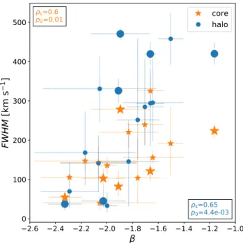
The most significant correlation is found between the width of the line and the UV continuum slope (calculated in H17) as shown in Fig. 11. This trend applies to the Lyα lines in the core (orange) and in the halo (blue) component (ρs' 0.75,
p0' 5 × 10⁻⁴). The β slope is known to be steeper for galaxies
with low dust content (Meurer et al. 1999), young stellar age or low metallicity. Our results may therefore suggest that more evolved galaxies, i.e., dustier, more metal-rich, and potentially more massive (Finkelstein et al. 2009;Yuma et al. 2010; Ono et al. 2010), show broader Lyα lines.
Finally, we find no correlation between the Lyα halo spec-tral profiles and the UV spatial extent of the host galaxies (i.e., rscore, see orange symbols in the first column of Fig. A.2).
The Spearman rank correlation coefficients of the two relations which are not shown in Fig. A.2 (FW H MHALO − rscore and
aasym,HALO− rscore) are (ρs = 0.36, p0 = 0.13) and (ρs = 0.09,
p0= 0.7), respectively.
7. Discussion
7.1. Diversity of the Lyα line profiles in the halo
This study allows for the first statistical analysis of the spectral signature of the Lyα emission in the CGM of LAEs. We find