On the Constancy of the Diameter of the Sun during the Rising Phase of Solar Cycle 24

HAL Id: insu-01176338

https://hal-insu.archives-ouvertes.fr/insu-01176338

Submitted on 7 Jul 2020

HAL is a multi-disciplinary open access

archive for the deposit and dissemination of

sci-entific research documents, whether they are

pub-lished or not. The documents may come from

teaching and research institutions in France or

abroad, or from public or private research centers.

L’archive ouverte pluridisciplinaire HAL, est

destinée au dépôt et à la diffusion de documents

scientifiques de niveau recherche, publiés ou non,

émanant des établissements d’enseignement et de

recherche français ou étrangers, des laboratoires

publics ou privés.

stancy of the Diameter of the Sun during the Rising Phase of Solar Cycle 24. The

Astrophysi-cal Journal, American AstronomiAstrophysi-cal Society, 2015, 808 (1), pp.808.4. �10.1088/0004-637X/808/1/4�.

�insu-01176338�

The potential relationship between solar activity and changes in solar diameter remains the subject of debate and requires both models and measurements with sufficient precision over long periods of time. Using the PICARD instruments, we carried out precise measurements of variations in solar diameter during the rising phase of solar cycle 24. From new correction methods we found changes in PICARD space telescope solar radius amplitudes that were less than ±20 mas (i.e. ±14.5 km) for the years 2010–2011. Moreover, PICARD ground-based telescope solar radius amplitudes are smaller than±50 mas from 2011 to 2014. Our observations could not find any direct link between solar activity and significant fluctuations in solar radius, considering that the variations, if they exist, are included within this range of values. Further, the contribution of solar radiusfluctuations is low with regard to variations in total solar irradiance. Indeed, wefind a small variation of the solar radius from space measurements with a typical periodicity of 129.5 days, with±6.5 mas variation.

Key words: space vehicles: instruments– Sun: activity – Sun: fundamental parameters – Sun: general – telescopes

1. INTRODUCTION

The Sun is an enormous ball of gas with a radius of 696,156 ± 145 km (Hauchecorne et al. 2014; Meftah et al. 2014c). Before the growth of astrophysics, the study of our star concerned mainly its geometric properties. This is why measurement of the Sunʼs diameter started as far back as antiquity, and Aristarque of Samos (∼310–230 B.C.) was the first to carry out measurements of the diameter of our star. Nowadays, the diameter of the Sun is a fundamental parameter used in physical models of our star. In particular, it could indirectly provideinformation about the amount of energy transmitted to Earthand thereforeabout the impact that this could have on our planetʼs climate. In fact, the only source of energy for the Earthʼs ocean-atmosphere system is the Sun. Any significant variation in this amount of energy could lead to a more or less direct variation in its average temperature due to the complexity of the climatic system in which ocean, atmosphere, aerosols, ground albedo, and biosphere are all likely to give rise to positive and negative feedback. This is why the study of variations in solar diameter is of particular interest. Is the solar diameter very much constant? Possible temporal variations of the solar diameter are of great interest for solar physics and climatology, e.g., as a mechanism for changes in total solar irradiance(TSI). Cyclic variability in TSI can be related to the corresponding changes in the solar radius R_e and effective temperature Teff of the Sun by deriving the Stefan–Boltzmann law. Thus, it is interesting to measure the changes in solar radius during an 11 yrcycle. If we assume that the variations observed over a solar cycle(∼0.1%) represent an upper limit for luminosity variation, and assuming no variation in temperature Teff, the greatest possible variation in the Sun radius ΔR_e cannot exceed 0.5 arcsec during a solar cycle. Periods of solar activity that are longer (the 87 yrGleissberg cycle or the 210 yrSuess cycle) than those of the solar cycle, lasting an average period of 11.2 yr, have been found and have

fueled discussion about the influence of solar variability on the Earthʼs climate (Braun et al.2005). The potential link between solar activity and variations in solar radius remains a matter of debate and requires models and measurements with sufficient precision over long periods of time.

Eddy & Boornazian (1979) were pioneers in the field of measuring solar radius variations. By analyzing Greenwich meridian transit measurements over a period of more than a century(1836–1953), they found a significant decrease in the solar diameter of around 0.1% per century. However, years later, by analyzing a larger data set covering 265 yr, Gilliland (1981) found a decrease of around 0.01% per century, or 10 times smaller than Eddy & Boornazian. Other analyses concluded that there has been no detectable change in the Sun over the course of the previous 250 yr(Parkinson et al. 1980). Hence, Shapiro (1980) argued that the solar radius had not decreased over time. Furthermore, Toulmonde collated all the solar radius measurements made between 1660 and 1995 and concluded that the mean solar radius at one astronomical unit is equal to 960.0 ± 0.1 arcsec. His research did notfind a substantial secular variation in the radius of the Sun(Toulmonde 1997). Nevertheless, it is extremely difficult to extract a trend in the Sun radius from historic data. Thus, the existence of any long-term trend in solar radius variability is still open to debate. In addition, studies of this variability during an 11 yrcycle or at least during a rising or descending phase of a solar cycle led to different results. Historic measurements of the solar radius carried out at the Calern site found anticorrelation with solar activity (Laclare et al. 1996) for a period covering solar cycles 21 and 22 (1978–1994). However, during solar cycle 23, ground-based measurements (with the solar astrolabe and Définition et Observation du RAYon SOLaire) found no clear correlation or anticorrelation between the solar radius and the activity of the Sun (Morand et al.2010). The Solar Disk Sextant (SDS) experiment, using seven balloon flights between 1992 and 2011, showed solar

showed that the solar radius can vary up to 0.2 arcsec (Sofia et al. 2013). However, the measurements carried out by the SDS reveal that the solar radius is not in phase with solar activity. Data collected by the Michelson Doppler Imager (MDI) on board the Solar and Heliospheric Observatory cover the whole of solar cycle 23 and show no sign of variations attributable to the 11 yrsolar cycle. Systematic changes in the solar radius with the sunspotcycle were found to be under 23 mas peaktopeak (Kuhn et al.2004; Bush et al.2010). The question thus remains open: does the solar diameter vary as a function of time, and is it related to solar activity? In order to ascertain this we now have at our disposal ground-based measurements, balloon measurements, and measurements out-side the atmosphere (space telescopes in orbit). Several measurements of the solar diameter were previously obtained by different methods(meridian transit, Mercury transit in front of the Sun, Venus transit in front of the Sun, astrolabes, imaging telescopes, eclipses, etc.). The measurementperiods differed, and the measurements themselves were carried out in spectral domains that varied from one instrument to another and contained the Fraunhofer lines susceptible to variability as a function of chromospheric activity. Thus, it is difficult to get a coherent picture on long-term trends from these results, and the subject is still a matter of debate.

Using measurements taken with instruments of the PICARD mission, we will determine the change in solar radius during the rising phase of solar cycle 24. We first present the developed mathematical methods and then discuss whether there is any significant correlation between solar diameter variation and magnetic activity during that period.

2. OBSERVATIONS

The PICARD program owes its name to Jean Picard (1620–1682), who is considered to be a pioneer of modern astrometry. The project involves not only a space mission but also a ground-based observatory at Calern (latitude N 43°44′ 53″, longitude E 6°55′36″, and altitude of 1271 m). Thus, measurements are taken in orbit by the PICARD mission satellite in order to avoid the impact of atmospheric effects. Nevertheless, it is important to understand and interpret the ground-based measurements, which actually constitute the longest series of currently available measurements. This is why an important ground-based measurement program (“PICARD SOL”) is associated with the space operation before, during, and after the PICARD space mission. The observationfields of the two instruments dedicated to the study of the Sun are summarized in Table 1.

Imager and Surface Mapper (SODISM) performed measure-ments of the Sunʼs diameter between 2010 August and 2014 March on the basis of an image of our star formed by a Ritchey–Chrétien telescope on a charge-coupled device (CCD). The main objectives of SODISM (Meftah et al.2014d) are as follows:

1. Measurement of the solar diameter at three wavelengths in the photospheric continuum as a function of helio-graphic latitude (at 535.7, 607.1, and 782.2 nm in the spectral bands excluding the Fraunhofer lines).

2. Detection of active regions (faculae and sunspots). The wavelength chosen corresponds to the emission of Ca IIat 393.37 nm, which is used also to measure differ-ential rotation.

3. Study of the effects of solar activity(solar image taken at 215.0 nm).

4. Study of the impact of active regions on the solar diameter.

5. Carrying out a deep Sun survey (using another filter at 535.7 nm dedicated to helioseismology study).

On the ground(at Calern, France), the SODISM II telescope has been carrying out complementary measurements since 2011 May. Ground-based observations of solar diameter are affected by the transit of photons in the atmosphere where scattering, turbulence, and absorption degrade the measure-ments. A turbulence monitor (Moniteur d’Image SOLaire Franco-algérien[MISOLFA]) was developed in order to characterize atmospheric turbulence. In addition, the data have to be corrected for astronomical refraction.

2.1. Problems Associated with Solar Diameter Measurements Measuring with precision the diameter of a gaseous sphere whose envelope is constantly changing represents a seemingly unachievable challenge, especially as the terrestrial atmosphere through which observations are made constitutes an immense handicap. To these difficulties are added the definition of the solar limb, which acts as a geometric reference point to demarcate the solar sphere. However, in spite of these hindrances, measurement of the solar diameter and its variations have been the subject of research programs in many observatories for many years. Indeed, the diameter of the Sun was a source of curiosity and study. Rozelot & Damiani(2012) gave a summary of efforts made since antiquity. The observations made outside the atmosphere are, in principle, more favorable. However, the effects of the space environment (ultraviolet [UV]effects, radiation, South Atlantic Anomaly, thermal cycling, etc.) leadto considerable degradation of the

instruments in orbit, which directly observe the Sun (combina-tion of the effects of contamina(combina-tion, radia(combina-tion, temperature variations, and detector responses). All these effects require correction(optical, thermal, electrical, etc.). On the ground, the instruments are far less affected by degradation processes and maintenance is possible. Nevertheless, measurements are affected by the atmosphere and require other types of correction (refraction, turbulence, etc.) that do not make it easy to obtain an absolute measurement of the Sunʼs diameter and to monitor variations in solar radius. Finally, the apparent solar radius is dependent on the distance between the Earth and the Sunand thus varies with the season. The amplitude of this distance effect is on the order of 25 arcsec on the solar radius. Measurements are thus corrected for this distance effect and are all adjusted to the distance of one astronomical unit(AU).

2.2. Measurements Carried out by PICARD Instruments Figure 1 shows the evolution of variations in solar radii observed at one AU by the two telescopes of the PICARD mission. We determined the solar radius from the inflection point position (IPP) of solar limb profiles taken at different angular positions of the image. The IPP for a given angular position is obtained by locating the zerocrossing of the second derivative of the solar limb profile. The mean radius is obtained from calculating all the inflection points of the different angular positions. For this study, we focused exclusively on observa-tions carried out in the solar continuum (535.7, 607.1, and 782.2 nm), in order to understand the spectral behavior of the telescope. The ground-based measurements carried out by the SODISM II instrument show the expected variations(impact of atmosphere on measurements). On the other hand, measure-ments carried out in orbit by SODISM show solar radius variations that are much greater than the expected order of magnitude (several milliarcseconds). The different measure-ments obtained from space show a temporal trend, which is wavelength dependent (this can be up to 3 arcsec on solar

radius variations). Moreover, the different variations associated with different wavelengths are not correlated. Understanding the source of this evolution is of major importance in order to correct the data obtained in orbit with SODISM.

2.3. Impact of the Space Environment on Measurements in Orbit

2.3.1. Evolution of the Intensity of Images Formed by SODISM

From 2010 August to 2014 March, SODISM collected more than a million images of the Sun at different wavelengths. Around 10 full-field, full-resolution images perday are produced in each wavelength. One of the primary roles of these images is to ensure a monitoring of the solar radius. From those images, we can also determine time series of the integrated intensities. Figure2 shows the long-term evolution in the normalized integrated intensity of images for each wavelength. This evolution in intensity is a function of wavelength and can go up to 95% of degradation for the spectral band centered at 215 nm. This change in transmission is not considered to be a major problem in itself with regard to the scientific objective of metrology associated with measure-ments of variations in solar diameter. In fact, it was compensated for by modifying the exposure time and change inflat field. Nevertheless, this evolution reveals a phenomenon, which has an impact on the performance of SODISM. For a given spectral band, there are alternating periods of decreases and increases in intensity. These variations do not seem to be correlated from one spectral band to another. These changes can only be explained by a modification in the optical properties of SODISM. We could suspect that the detection pathway (detector, reading circuit, post-processing, etc.) also plays a role in this change. However, the observed phenom-enon is wavelength dependent without following a monotone evolution. The hypothesis of a modification in optic config-uration that highlights interference effects is therefore the preferred option. Thus, the only remaining hypothesis is Figure 1. Top:evolution of raw solar radius variability over time (measurements in orbit). This shows the impact of space environment on measurements carried out by the SODISM instrument. Bottom:evolution of raw solar radius variability over time (measurements on the ground). This shows the impact of atmosphere on measurements carried out by the SODISM II instrument.

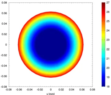
contamination of the optical surfaces operating in transmission (contamination of the front window and/or contamination of interference filters). Generally, the first optical surface of a space instrument exposed to the Sun corresponds to the surface, which will suffer degradation before any other optical element. In the follow-up to this study, we will focus on analysis of SODISMʼs front window contamination effects, characterized by an increase in the temperature T r t( , ) of this fundamental optical parameter. Computer-aided design representation of the SODISM telescope is shown in Figure 3, where the front window subassembly is represented. The appearance of the temperature gradient(ΔT) is represented in Figure4.

2.3.2. Temperature Evolution of the SODISM Front Window

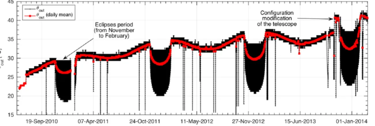
The temperature (θout) of the front window mechanical interface evolves over time (Figure 5). This change in temperature reveals contamination over the course of time of the telescopeʼs optical surface (modification of thermo-optical properties[αf] of the front window induced by effects such as solar flux absorption). Just before the end of the PICARD space mission (2013 November), we modified the telescope configuration (modification of a temperature set point, which leads to the evolution of the front window radiative environ-ment). From that moment, the temperature θout changed significantly. Similarly, we observed a change in solar radius variability after that event(Figure 1). This clearly shows that there is indeed a relationship between the front window temperature and the evolution of the raw solar radius (Irbah et al.2014). We wish to point out that these variations in solar radius are slow and not associated with noise.

2.3.3. Impact on SODISM Observations

Owing to the increase of the space instrument degradation, the final results will be given from 2010 August to 2012 December(for a more extensive explanation, see Section4.2). 2.4. Impact of Atmosphere on Ground-based Measurements

The main causes of disturbance acting on solar images are related to the transparency of the atmosphere and to turbulence effects (modifying the apparent mean solar radius up to over 1 arcsec). The installation of complementary instrumentation (photometer, pyranometer, and wide-field camera) provided us with additional information.

3. MODELS

The observations that contribute to build the model are as follows:

1. Mechanical interface temperature of the front win-dow(θout).

Figure 2. Normalized time series of integrated intensity from the beginning of the PICARD mission (normalized transmission tλ of the telescope at a given wavelength). The degradation is considerable in the UV spectral bands.

Figure 3. Location of the front window at the telescope level.qoutrepresents the front window interface temperature, and r is the radial coordinate.

Figure 4. Front window temperature gradient (ΔT = 9°C). Under this scenario, the front window temperatures (T(r, t)) ranged between 18°C and 27°C.

2. Normalized time series of integrated intensity at each wavelength.

3. Evolution over time of the absorbed solar flux and absorbed infrared (IR) flux.

4. Evolution of the uncorrected solar radii at one astronom-ical unit for each wavelength.

3.1. Models Associated with the Space Instrument SODISM

3.1.1. Optical Model

In the previous section, we noted that the temperature of the front window T r t( , ) could have an impact on solar radius measurements. We therefore developed an optical model in order to better understand the phenomena we had observed during the PICARD space mission. In fact, modification of the optical wavefront can disrupt the measurement. The wavefront w0corresponds to the sum of all Zernike polynomials Zk(ρ, θ) combined with the terms Ck.

w C Z ( , ) (1 )a k k k 0 1 36

å

r q = ´ = C D f n T h T b 16 1 2 ( ) (1 ) w f 3 PS 2 S 2 d l l a = ´ ´ ´ + ´ ´ ¶ ¶ ´ ´ D n T A0 A1 exp B1 A exp B , (1c) 2 2 l l ¶ ¶ = + ´ æ è çç çç- öø÷÷÷÷+ ´ æ è çç çç- öø÷÷÷÷

whereρ and θ represent cylindrical coordinates. C3corresponds to a focus term associated with de-focalization of the image plane(δ) and to a radial temperature gradient in the telescope front window (ΔT(αf)). DPS represents the diameter of the telescope pupil (90 mm), fScorresponds to the telescope focal length (2629 mm), λ corresponds to the observation wave-length (in nm), hw represents the thickness of the telescope front window, and n

T

¶

¶ (ppm K−1) corresponds to the variation in

the useable wavelength indices(for silica: A0= 8.241466462, A1 = 524.4619629, A2 = 7.836746871, B1 = 45.22476821, and B2= 211.2250895). The term C9, combined with Zernikeʼs

polynomial Z9, corresponds to an astigmatism defect(As). The complex wavefront W takes into account central obstruction (A_DPS is a surface limited by the telescope spiders and

secondary mirror mask). The SODISM point-spread function (PSF) depends on the complex wavefront W(px, py). The line-spread function(LSF) is obtained by integrating over the PSF columns. We carry a convolution(symbol ⊗) of the LSF with the desired theoretical solar limb profile HM98 (see Hestroffer & Magnan 1998), where LDF r( ,S l represents the limb-) darkening function(rSrepresents the Sunʼs radial coordinates, andαS(λ) is a parameter given by the HM98 model, which is wavelength dependent). Whatever the solar profile used, when we have a significant defect (radial temperature gradient, focus, astigmatism, etc.), the PSF represents the predominant factor in our calculation. These relationships reveal the complexity of our system and the many parameters associated with it:

(

)

W p px, y =ADPS ´e2i w0 (2 )a p ´ ´

(

)

(

)

x y W p p e dp dp b PSF ( , ) , (2 ) x y i x p y p x y SODISM 2 _{x y}

ò

ò

= ´ p -¥ +¥ -¥ +¥ ´ ´ ´ + ´

(

r

)

r c LDF S, 1 S2 (2 ) ( ) S l = - a l

(

)

x y dy r d LDF PSF ( , ) LDF , . (2 ) y y SODISM SODISM S 1 2

ò

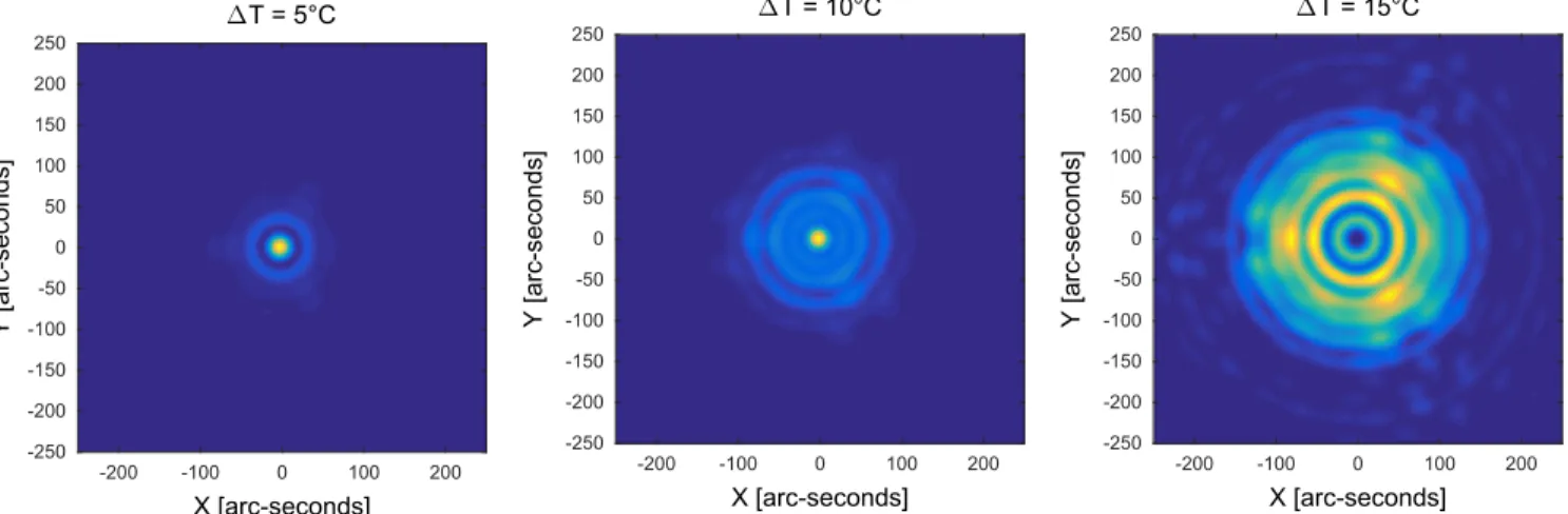
l = Ä

Using the optical model (see Equations (2a)–(2d)), we can determine the theoretical PSF of our telescope at a given wavelength and for a given temperature gradient. The effect of a temperature gradient on the PSF of our telescope at 782.2 nm is shown in Figure6. The change in thefirst derivative of the solar limb at 782.2 nm convolved to the PSF of the instrument is given in Figure 7 (LDFSODISM). These various simulations show the sensitivity of our telescope when it is subjected to a temperature gradient. Finally, evolution of the solar radius as a function of the temperature gradient can be seen in Figure 8 and reveals the dependency with wavelength.

3.1.2. Thermal Model

In this section, we will establish the equation for the temperature of the SODISM instrument front window as a function of the various inputfluxes. As stated in the previous section, the temperature of the telescope front window has a major impact on the instrumentʼs performance. This model is Figure 5. Evolution of the front window mechanical interface temperature (θout). The front window temperature (T(r, t)) depends on the mechanical interface temperature(θout). Around two milliontemperatures were recorded (black curve with dots).

necessary and explains the variations in solar radius observed with the space instrument of the PICARD mission. It is thus important to characterize the evolution of the temperature range of the front window over time, and this is why we wanted to set up a numerical model. The front window temperature(T(r, t)) is a function of the radial coordinate r(Figure3). To simplify the calculations, we will assume that we have the context of

ahomogeneous isotropic material, where it can be assumed that the thermal conductivity coefficient of the material (Λ) is constant and independent of both the spatial variables and time (data depending on daily mean parameters). It consists of a circular silica disk of limited thickness (hw = 8 mm) and an external radius of 57 mm (Rf = rout). Considering a small element of volume dV= 2πr × dr × hw of our front window, Figure 6. Evolution of SODISM telescope PSF for different temperature gradient values (ΔT = 5°C, 10°C, and 15°C) at the front window.

Figure 7. Evolution of the solar limb first derivative LDFSODISMas seen by the SODISM instrument(from the LDF of the Sun convolved with the instrumentʼs PSF). Left:effect of a temperature gradient (ΔT). Right:effect of a temperature gradient (ΔT) combined with an astigmatism defect (C9= −0.25).

Figure 8. Left:evolution of the solar radius (determined by the inflection point method) as a function of a temperature gradient (ΔT) for different wavelengths. Right:ΔT effects combined with an astigmatism defect (C9= −0.25) on solar radius measurements.

where dr represents a ring element, and placed in a temperature range characterized at all points by a given vector grad T , and after solving the differential equation, we obtain

T r t T t T t C t J i r C t C t Y i r C t a ( , ) Flux( ) ( ) ( ) ( ( )) ( ) ( ( )) (3 ) it b 1 out 1 0 2 0 e s = + ´ ´ + ´ ´ ´ + ´ ´ ´ + ¥ t t t fv t t t fv t t b Flux( ) ( ) ( ) ( ) ( ) ( ) ( ) ( ) (3 ) f ir f a A S out IR a j e j a j = ´ + ´ ´ + ´ ´

(

)

(

)

T t( ) = T¥+T r tit( , ) ´ T¥2 +T r tit( , )2 (3 )c C t T t h d ( ) b ( ) (3 ) w out e s = ´ ´ L ´

(

)

(

)

(

)

(

)

(

)

(

)

(

)

C t t Y i r C t J i r C t Y i r C t J i r C t Y i r C t e ( ) ( ) ( ) ( ) ( ) ( ) ( ) (3 ) c c c 1 out 1 1 0 out 0 out 1 q = - ´ ´ ´ ´ ´ ´ ´ ´ - ´ ´ ´ ´ ´

(

)

(

)

C t C t J i r C t Y i r C t f ( ) ( ) ( ) ( ) , (3 ) c c 2 1 1 1 = - ´ ´ ´ ´ ´

where the sum of the absorbedfluxes by the front window is represented by the parameter“Flux,” which evolves over time. Emissivity ɛout takes into account the capacity of the material on the external side of the window to emit energy by radiation toward cold space(4 K), whose temperature corresponds to T¥.

σb represents the Stefan–Boltzmann constant. The telescope front window is subjected to external fluxes such as solar flux (ϕS), infrared flux (ϕIR), and albedo flux (ϕA). The PICARD satellite permanently observes the Sun (outside of eclipse periods). The view factor between the Sun and the external side of the front window of SODISM is equal to 1. The relative position of the external side of the front window with respect to the Earth evolves during an orbit and over time. The view factors fvirand fvAtake into consideration this effect. J0, J1, Y0, and Y1represent Bessel functions J and Y of order 0 and order 1;rc represents the internal radius of the front window and tends toward 0 (numerical stability of calculation). The

imaginary unit is represented by i. This model is associated with an iterative process(it).

Using the thermal model, we can determine the evolution of the front window temperature gradient over time. Starting with values measured in the laboratory (αf = 0.14 and ɛout = 0.81)and assuming that no degradation of our system takes place (αf is constant), ΔT(αf) can vary from 10°C to 14°C (Figure9). This variation is related to the evolution over time of the front window temperature interface(see Figure5). These temperature gradients have a significant impact on the PSF of the telescope and on the performance of our system(see Figure 8). They cause a shrinking back in the IPP of the measured solar radius (value below 957 arcsec) whatever the observation wavelength. This model shows the criticality of our optical configuration when it is subjected to a temperature gradient, which is difficult to characterize on the ground (environment tests on space instrumentation). A thermal vacuum test with a solar simulator does not allow us to identify this type of effect. In fact, the sensitivity of our system is manifested through parameters, which vary with time (αf varies[contamination], absorbed IR flux varies, etc.).

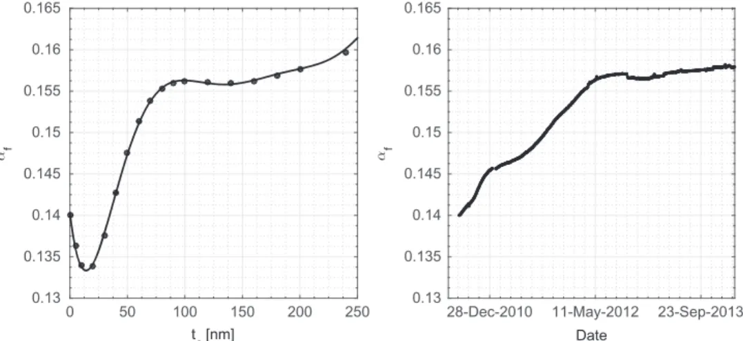
3.1.3. Model Associated withαfCoefficient Determination In order to characterize our system, we developed a model allowing us to estimate evolution of the solar absorption coefficient (af) over time (Appendix A). Evolution of the

intensity of the images formed by SODISM can be explained by contamination of the front window(glass indices: n = 1.46 and k= 4.2 × 10−8). With regardto the nature and physico-chemical origin of the contamination, this can be a derivative of carbon(indices: n = 2 and k = 0.1) or a derivative of silicone. By varying the thickness of the contaminating layer, the transmission τ(λ) of our front window can change. We can thus calculate the change inαfas a function of the thickness of the carbon contaminant (Figure 10). Similarly, using the intensity of images formed by the telescope, we estimated the evolution ofαfover time(Figure10). This evolution leads to a change in the temperature T(r, t) of our telescope.

3.1.4. Mechanical Model

In order to characterize the mechanical effects on the optic wavefront, we created a mechanical model. We therefore considered the telescope window to be a thin disk subjected to Figure 9. Left:evolution over time of the solar flux (orbital mean) absorbed by the front window (ΦS= αf×ϕS). Middle:evolution of the IR flux absorbed by the front window(ΦIR= òout× fvir×ϕIR) for different values of the albedo (seasonal and spatial evolution of albedo [a]). Right:evolution over time of the front window temperature gradient( TD ) for different values of the solar absorption coefficient (αf).

a radial temperaturefield T(r, t). The displacement field u(r, t) can be expressed as follows:

u r t r T r t r dr r r T r t r dr ( , ) (1 ) ( , ) (1 ) ( , ) , (4) m r r 0 2 out 2 ₀ out

ò

ò

a n n = ´æ_{èçç +} ´ ´ + - ´ ´ ´ ö ø ÷÷÷ ÷÷ where αm represents the thermal dilatation coefficient of the optical material(0.5 × 10−6 K−1) and ν represents the Poisson coefficient, which is equal to 0.17. The temperature field generates a displacement field, which has a negligible impact on the wavefront and on instrument performance. In fact,αmis very weak, and therefore the thermo-elastic effects on telescope performance are very limited (a few mas).

3.1.5. Thermal Modelʼs Limitations

Thermal models range from simple, steady-state simulations to complex, transient,finite element method (FEM) codes with tens of thousands of nodes. The models are very useful in that they provide a straightforward means to incorporate the numerous physical variables that affect our solar radius measurements. Our modelis applied to complex situations. Upon setting up the proper boundary conditions and homo-geneous isotropic material properties (constant thermal

properties, except forαf), the temperature field at front window level was calculated. Our thermal model has limitations, which include the accuracy of the inputs to the model. The main inputs are the mechanical interface temperature of the front window (accuracy impact), the absorbed solar flux (TSI absolute value knowledge impact), the absorbed IR flux (impact of variations during an orbit from 30 to 60 W m−2_), and the evolution of the solar absorption coefficient (Daf

variations impact). Our thermal model has another limitation, which is related to the model that is valid for steady-state simulations. The adopted hypothesis (steady-state model) shows the limitation of our model during the eclipses. In the case of a transient model, the computation time would be very long. Indeed, around two million temperatures (θout) were recorded. Moreover, we need to use the data (IR flux and albedo fluxes) provided by the National Oceanic and Atmo-spheric Administration. Finally, a complex FEM would be more appropriate for a transient case.

3.1.6. Modelʼs Uncertainties

Uncertainties of the model are given in Table 2. Spectral reflection ( ( )0 l ) and transmission (τ0(λ)) measurements

were performed with a spectrophotometer(Agilent Cary 5000 UV-NIS-NIR). The estimated tolerances are expected to be less than ±1%. Solar absorption (A0(λ)), depending on the wavelength, is given by Meftah et al. (2014d). From these Figure 10. Left:evolution of solar absorption (αf) obtained as a function of the thickness (tc) of a carbon contaminant (using the Thin Film Calculation program). Right:evolution of solar absorption (αf) obtained from normalized telescope transmissions tλ. This variability(Daf) is weak (mainly degradation in UV) but has an

enormous influence on the performance of our telescope.

Table 2 Model Uncertainties

Uncertainty Sources Typical Values Uncertainty Error onDT(oC) Uncertainty Type

f

a a

0.140 ±0.001 ±0.10 Test(S) and aging (R)

out e b 0.81 ±0.01 ±0.30 Test(S) Lb 1.38 W m−1K−1 ±0.04 W m−1K−1 ±0.31 Test(S) out

q a _22.00o_{C ±0.10 ±0.03 Calibration and measurement(S)}

S jc _{1,362.1 W m}−2 _{±2.4 W m}−2 _{±0.02 Measurement(S)} IR j c 238.0 W m−2 ±6.0 W m−2 ±0.02 Literature(S and R) A j c ∼20.0 W m−2 _{±9.0 W m}−2 _{±0.02 Literature(S and R)}

Note. Some uncertainties may be considered random (R), while others are systematic (S). a

Parameter that varies over time, which is subject to the effects of instrumental degradation. b

Parameter that remains constant. c

±2.4 W m (Meftah et al. ). Linked to the satelliteʼs position (view factor impact), the other parameters have a limited effect(ϕIRandϕA). Thus, they do not require a great accuracy. Thus, in closing, these measurements make it possible to establish a model uncertaintybudget. While the systematic uncertainties affect only the absolute measurements, random uncertainties affect the absolute and relative measure-ments. Therefore, random uncertainties have an impact on the correction model of the solar radius variations.

3.2. Models Associated with the SODISM II Ground Instrument

3.2.1. Refraction

Astronomical refraction (Ref) influences the solar radius measurements (more than 1 arcsec for observations made above 70° of zenith distance z) that we obtain from images taken with SODISM II. In fact, the heliographic latitude of the observed solar diameter changed during the year as a result of the inclination in the Earthʼs orbit along an ecliptic plane and the inclination of the axis of solar rotation. We therefore use a numerical method to correct mean solar radius measurements at whatever wavelength(λ). This correction also depends on air temperature (Ta), pressure (Pa), and relative humidity (fh). In order to quantify the effect of refraction at the observatory position, we can incorporate the length of the trajectory of the rays from the local refractive index of the atmosphere n= nobsand the local zenith distance ξ = z at the observatory position, and this up to n = 1 (beyond the atmosphere). An approximate formula for correction is given in Equation (5b), which shows the relationship between the corrected solar radius for refraction(Rcor), the observed solar radius (Robs), and the refraction correction coefficient (Cref(Ta, Pa, fh,λ, z)):

dn n a Ref tan (5 ) n 1 obs

ò

x =

(

(

)

)

Rcor Robs Cref T P fa, a, h, ,z (5 )b 1 l ´ -

(

)

(

)

(

)

C T P f z k T P f z c , , , , 1 , , , 1 0.5 tan ( ) (5 ) a a h a a h ref 2 l = - l ´ + ´

(

)

(

) (

( )

)

k T P fa, a, h,l =ar T P fa, a, h,l ´ 1-b Ta , (5 )d

where ar( ,T P fa a, h,l is the air refractivity for local atmo-) spheric conditions at a given wavelength(Ciddor1996), and β (Ta) (see (AppendixB)) is the ratio between the height of the equivalent homogeneous atmosphere and the Earth radius of curvature at observer position assuming the ideal gas law for dry air(Ball1908). In our calculation, we used a mean value of k(Ta, Pa, fh,λ).

Kolmogorov statistic with that of a smaller telescope but affected only by light diffraction(if it is in space, for example). The Fried parameter (r0) corresponds to the equivalent diameter of such a telescope limited by diffraction (entirely circular pupil of diameter DPS). This is why one of the objectives of the MISOLFA instrument is to quantify the effects of atmospheric turbulence on measurements of solar diameter carried out by SODISM II. Thus, taking into consideration the Kolmogorov model, r0 is related to angle-of-arrivalfluctuationvariances_a2 (Borgnino et al.1982) by

( )

r0 8.25 105 DPS . (6) 1 5 6₅ 2 3 5 l s = ´ ´ - ´ ´ _a

-We used this equation to determine r0at a given wavelength (measurements carried out using MISOLFA at 535 nm with DPM= 25 cm). We note that r0is dependent on the wavelength and proportional tol . This dependence is the reason why the65

wavefront is relatively less phase disrupted for the longer wavelengths. The change in FWHM of the first derivative of the solar limb observed by SODISM II (Figure 13of Meftah et al.2014aat 535.7 nm, and Figure11at 782.2 nm) can also be used as a relative indicator of turbulence given the relationship between the FWHM and the pupil diameter DPS. This indicator is relative because a small defect in the telescope optics such as a triangular astigmatism produces a bias in the SODISM observables(Figure12).

4. RESULTS AND DISCUSSION

SODISM has taken more than one million images of the Sun at several wavelengths. The replica of the space instrument (SODISM II) installed at the Calern site has taken more than 100,000 measurements of the solar radius at several wave-lengths over a period of more than 3 yr. Using measurements carried out by instruments on the PICARD mission, we established the variations in the solar radius during the rising phase of cycle 24. Moreover, we also investigated correlations between solar activity, measurements of TSI, andfluctuations in the radius of our star. The TSI varies over a number of different timescales ranging from several minutes to several decades(a daily variability can reach peak-to-peak amplitudes of around 0.3%, a variability of around 27 days that is a function of the evolution of sunspots and faculae, a variability of around 11 yrwith an amplitude on the order of 0.1%, etc.). Could we attribute part of the variations in TSI to variations in solar radius? The precision of measurements is a critical point that requires space observations to be used since the terrestrial atmosphere constitutes an impediment (see ground-based measurements obtained with SODISM II;Figure 1). In spite

of these observations outside the atmosphere, we were able to note that the space environment (UV effects, contamination, thermal cycling, etc.), combined with initial defects in telescope calibration(astigmatism, position of the focal plane, etc.), can considerably degrade the measurements taken by our instrument (see measurement obtained with SODISM;Figure 1). The various observations we carried out on the ground and in orbit reveal the usefulness of the developed models (see Section 3) for data correction. In addition, we found that images taken at 782.2 nm were relevant both on the ground and in orbit, and this for different reasons (wavefront of ground-based measurements less subject to phase disturbance by turbulence in the higher wavelengths, and impact of tempera-ture gradient of the space telescope window on PSF lower at 782.2 nm).

4.1. Solar Radius Measurements Obtained by the PICARD Ground-based Facility

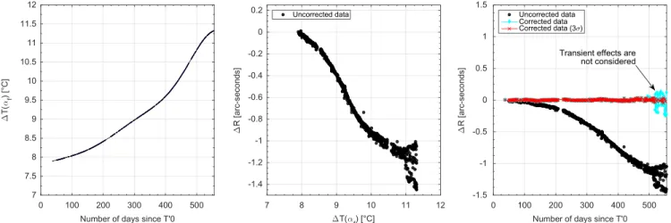
Using the different images acquired by the SODISM II instrument, we calculated the observed mean solar radius. It is determined by the IPP of the solar-limb profiles taken at different angular positions of the image. The results presented in Figure13(uncorrected data, on the left) were obtained from images acquired at 782.2 nm. The results that we obtain for other wavelengths are similar(Meftah et al.2014a). They show daily variations of the observed solar radius that are higher at 535.7 nm and at 607.1 nm than at 782.2 nm (effect of

turbulence where r0 is proportional to

6 5

l ). The IPP can be obtained from the different solar models. The differences (ΔIPP) in the IPP at 607.1 nm and at 782.2 nm with respect to a reference position at 535.7 nm are relatively small—roughly 30 mas for 782.2 nm, regardless of the solar model used (Table 3). Consequently, the measurements carried out at 782.2 nm are considered as baseline measures. One of thefirst steps consists in eliminating aberrant measurements through data analysis and in correcting refraction effect data (see graph in the middle of Figure 13). The data selection is explained in more detail by Meftah et al. (2014a). Aberrant measurements were identified as originating from incomplete images(pointing, etc.) and data contaminated by atmospheric effects. Over 25,000 measurements have been made at 782.2 nm since 2011 May. A measurement is obtained from calculating over 4000 inflection points of an image as a function of the angular position(θ). During a day, the various solar radius measurements observed on the ground and corrected for refraction can vary by up to±0.5 arcsec. Among other things, these variations correspond to the effects of turbulence. By analyzing the change in the solar limb first derivative FWHM at 782.2 nm over time(Figure11), we find evidence of cyclicalfluctuations during the course of the year (mean FWHM at 782.2 nm is near 7.6 arcsec). The fact that these cyclicalfluctuations are found to be similar from one year to the next allows us to confirm the stability of our device (very slight instrumental drift). In order to reduce the effect of daily Figure 12. Impact of a 19 nm rms triangular astigmatism defect of the telescope (As1) and of a 57 nm rms defect (As2). Evolution of the solar limb first derivative FWHM for different wavelengths(535.7 nm, left panel;607.1 nm, middle panel;and 782.2 nm, right panel) as a function of the telescope pupil diameter (DPS), which is comparable to the Fried parameters(r0).

variation in turbulence, we first take daily mean values from our data (right-hand graph in Figure 13). Additionally, we estimate that the Fried parameter is between 2.3 and 7 cm at 782.2 nm (relationship among the solar limb first derivative FWHM that it is measured by SODISM II, the pupil diameter DPSof the telescope equated to r0, and the possible astigmatism defect). Similarly, we have a measure at 535.7 nm of the solar limb first derivative FWHM considered near 8.6 arcsec (see Figure 13of Meftah et al. 2014a). Thus, we estimate that the average Fried parameter is between 2.3 and 3.7 cm at 535.7 nm (see Figure 12 to better understand the likelihood of astigmatism defect). This result is similar to the one we obtained using measurements performed by the MISOLFA instrument. In this study, we are not interested in absolute determination of the solar diameter (impact of measurement bias) but rather in variations in solar diameter over time. Daily mean solar radii are obtained from measurements that are derived from different atmospheric conditions. However, the solar limbfirst derivative FWHM at 782.2 nm shows no sign of change for long-term measurements. Thus, the monthly averages of solar radii are excellent indicators for our measurements. Finally, we carry out monthly averages of the observed solar radii (on the right in Figure13). At the start of 2014, the weather conditions were very bad and observations were very limited. We can see the effects of these conditions on our monthly averages of solar radii(Figures 13and 18). The operationrepeatability is important, as is the SODISM II instrumental stability. The SODISM II solar radius at 782.2 nm shows amplitudes (cloud of points) below ±50 mas

after 40 months of measurement(Figure18). The trend of our measurements during the period 2011–2014 shows a solar radius evolution below 25 mas(tendency with a nonsignificant negative slope). This result requires a more detailed analysis (turbulence affects impact, etc.). Indeed, the trend may be of solar origin, of instrumental origin, of atmospheric origin, or a combination of the three.

4.2. Solar Radius Measurements Obtained by PICARD Space Mission

Using various images acquired by SODISM, we calculated the value of the observed mean solar radius over time. The different measurements taken show a temporal drift that is a function of wavelength(see Figure1). As stated in the previous sections, a temperature gradient in the telescopeʼs front window greater than 5°C leads to significant variations in solar radius measurements related to degradation of the telescopeʼs PSF (Figure 8). Thus, on the basis of optical coating degradation evaluation by a contamination effect (αf variations), we estimated the evolution of the temperature gradient in the SODISM front window over time (Figure 14). Temperatures range from 8°C to 11.5°C. These temperature variations are compatible with those we calculated(Figure 9) when αfwas taken to be constant. Thus, the slow variations in solar radius observed by SODISM can only be explained by instrumental effects associated with a temperature gradient in the telescope front window and by initial calibration errors. In fact, comparison with the very good measurements taken on the ground demonstrates this state of affairs. Similarly, the spectral effects that we observe are not in phase and can be explained by a temperature gradient, in accordance with the models, which we developed in Section 3.1. Consequently, we can consider SODISM to be a very good indicator of variation in solar radius for short-term period, contrary to SODISM II. The ground instrument is subject to atmospheric effects(short-term, medium-term, and long-term effects) but remains instrumen-tally stable with time, whereas SODISM is subject to the effects of the space environment (long-term effects). For SODISM, more the wavelength of observation is great(e.g., at 782.2 nm) and more the instrumental effects on the PSF (front window temperature gradient impact) are reduced. Similarly, for SODISM II, more the wavelength of observation is great and more the effects of atmospheric turbulence are less important Figure 13. Evolution of the solar radii at one astronomical unit (uncorrected [left panel]and corrected [middle panel]) since the first measurements carried out by SODISM II in 2011 May(T0). Right:daily and monthly averages of the corrected solar radius evolution.

Table 3

Difference(ΔIPP) of the Position of the Inflection Point Position at 607.1 nm and 782.2 nm with Respect to the Reference Position at 535.7 nm(for

Different Solar Models)

Solar Models 607.1 nm 782.2 nm

ΔIPP VAL81 11.9 mas 30.2 mas

ΔIPP FCH09 13.6 mas 32.8 mas

ΔIPP COSI 10.0 mas 28.0 mas

ΔIPP SH09 9.4 mas 21.2 mas

Note. Some models use theoretical approaches, such as VAL81 (Vernazza et al. 1981), FCH09 (Fontenla et al. 2009), and COSI (COde for solar

irradiance;Shapiro et al. 2010). Others are based on physical principles

(turbulence bias on solar radius measurements). In the PICARD case, the channel at 782.2 nm is optimal. We highlight the importance of ground-based and space measure-ments. Indeed, our measurements show the benefit of simultaneous measurements obtained from ground and space observatories. As a result, these two means are complementary to each other and represent a feedback for solar observations. We therefore focused in particular on SODISM measurements taken at 782.2 nm. The correction of the solar radius, which is associated with slow drift of our measurements, is shown in Figure14(right panel). The cyan curve in Figure14shows the evolution of the solar radius obtained after applying the temperature correction(Figure14, left panel) connected to the solar radius adjustment (see Figure 8). The transient effects observed during eclipses are not taken into account in our model(thermal modelʼs limitation). We thus filter data at 3σ in order to obtain an evolution that corresponds to the stabilized phases of our instrument. Figure 15 gives the evolution of SODISM solar radius, together with associated uncertainties that increase over time. The cloud of points (solar radius measurements) is then fitted by a sinefunction with a frequency, an amplitude, and a phase. The goodness of the fit is excellent(R2coefficient of determination of 0.97).

Peak-to-peak amplitude of the solar radius fit is close to 13 ± 1 mas (statistical uncertainty with 95% confidence bounds). More-over, the obtained results highlight a periodicity of 129.5 ± 1.0 days. In 2012, this periodicity is difficult to detect (Figure 16). In closing, SODISM solar radius amplitudes (cloud of points) are smaller than ±20 mas (i.e. ±14.5 km) for the years 2010–2011.

By the end of 2011, the variations of the solar radius during an orbit become more important. Similarly, periods of eclipses from 2011 November have a significant impact on the variations of the solar radius (Figure 1). In late 2011, the deterioration in the UV band (Figure 2) is significant (more than 90% at 215.0 nm). In late 2011, the front window mechanical interface temperature (θout) continues to increase (about 35°C), which is between 20°C and 35°C during periods of eclipses between 2011 November and 2012 February (Figure 5). But what is most criticalis that the temperature gradient of the front window has found a balance between 10°C and 12°C. This temperature gradient range corresponds to an unstable region of the solar radius determination (Figure 8, right panel). Indeed, in this temperature gradient range, determining the inflection point is more complex (Figure7). In addition, from mid-2011, the uncertainty of the temperature Figure 14. Left:evolution of SODISM front window temperature gradient (obtained from the steady-state thermal model). Middle:relation between temperature gradient and uncorrected solar radii at one astronomical unit. Right:evolution of the solar radii at one astronomical unit (uncorrected and corrected) since the first measurements carried out by SODISM in 2010 August(T′0).

Figure 15. Evolution of daily mean solar radius measured by SODISM, together with associated uncertainties. The evolution is given by the continuous red line (sinusoidal fit). The period of 129.5 days is clearly observable in 2010 and 2011.

gradient determination increases significantly (Figure15). This demonstrates that the problem is not trivial and requires a more detailed analysis during this period.

4.3. Source of Signal Taken by Both Instruments PICARD ground-based and space observatories represent a joint venture to study the Sun. Thus, we need to establish data linkages with SODISM and SODISM II. Figure 16 gives PICARD solar radius variations based on the monthly averaged values. Through these data, there is no significant common source of signal taken by both instruments. Pearsonʼs correlation coefficient (kp) between SODISM and SODISM II solar radius variations is near 0.1. Similarly, Pearsonʼs correlation coefficient between SODISM solar radius variations and monthly mean sunspot numbers is close to 0.04. Moreover, there is a very low decreasing linear relationship (antic-orrelation) between SODISM II solar radius variations and monthly mean sunspot number. However, this relationship is not clearly defined (kp= −0.14). To better analyze the signal taken by both instruments, we also used spectral analysis. In order to further look for periodicities, we computed the Lomb– Scargle (Lomb 1976; Scargle 1982) periodograms using the full time series of SODISM and SODISM II solar radius measurements. The Lomb–Scargle periodogram analysis is a commonly used first approach for spectral analysis of uneven time series. Its main interest is that it avoids the use of interpolation or any other means offilling the gaps, which are needed when applying a classical Fourier transform. In Figure17, we show the two Lomb–Scargle periodograms with estimates of significance levels against the null hypothesis of random noise. For space data covering years 2010–2011 (SODISM), the peak around 129 days of periodicity, already obtained from our sine-wavefitting, is found to be significant at the 99% confidence level. There is also a periodicity around 38 days (99% confidence level) associated with solar radius variation of very low amplitude (±2 mas). For ground-based data, covering years 2011–2014 (SODISM II), only one peak for periodicity around 82 days is found to be significant at the 95% confidence level. A periodicity around 27 days, corre-sponding to the synoptic solar rotation rate, was previously found in the analysis of Calern and Rio Astrolabe measure-ments over cycles 21, 22, and 23 (Moussaoui et al.2001; Qu

et al. 2015). This periodicity is not found to be significant in our analysis of both space- and ground-based full-time data over the rising phase of cycle 24. The periodicity around 82 days has previously been interpreted as a possible second harmonic of the rotation rate. However, without significant signal for the main peak (27 days) and first harmonic (54 days), this interpretation is doubtful in our case. The interpretation of the only significant periodicity around 129 days found in the SODISM space data is not obvious, but we notice that a similar periodicity hasbeen reported in solarflare occurrence during cycle 23 (Bai2003) and a close periodicity was found in the frequency shifts of low-degree p-modes over cycle 22 and the rising phase of cycle 23 (123.7 days;Salabert et al.2002). In the Calern Astrolabe solar radius measurements over cycles 21 and 22, a periodicity of 122.3 days was also found to be significant by Moussaoui et al., but it was not found by Qu et al.(2015) in their analysis of the Rio Astrolabe data over cycle 23. This is afirst attempt to look for high-frequency signal in our new time series of ongoing radius measurements covering more than 4 yr. With the main periodicity for solar activity being around 11 yr,it is clear, however, that we have to wait for a longer homogeneous time series, over which we will be able to perform more detailed spectral analysis.

4.4. Fluctuations in the Solar Radius as a Function of Solar Activity

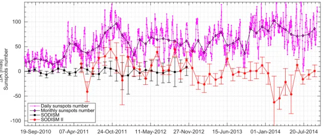
From PICARD measurements and models, we can determine solar radius fluctuations as a function of solar activity during the rising phase of cycle 24(Figure18). This particular cycle is the smallest since solar cycle 14. Our ground-based observa-tions (2011–2014 period) could not find any direct link between solar activity and significant fluctuations in solar radius(with amplitudes around ±50 mas). In fact, we find no relationship between the significant fluctuations in solar radius and the change in the TSI, which is connected with the number of sunspots. By contrast, measurements taken by SODISM (2010–2011 period) highlight a ±6.5 mas variation in the solar radius with a periodicity of 129.5 ± 1.0 days. However, no significant variation of the solar radius (greater than ±20 mas) has been observed. Thus, there is no direct link with solar activity for significant variation of the solar radius for the years Figure 16. Evolution of monthly mean solar radius variations (SODISM and SODISM II) vs. daily and monthly mean number of sunspots. Error bars represent statistical uncertainty at 1σ. The period of 129.5 days is not clearly visible in 2012, where the dispersion of the data in this period is greater.

2010–2011. Moreover, we obtain overlapping results between those obtained by SODISM and those obtained by SODISM II. After 2012, the amplitudes measured by SODISM are greater owing to the increase of the instrument degradation. The rising phase of solar cycle 24 became apparent as of 2011, a period in the course of which we have useable observations, and where no significant relationship with TSI is detectable. The study of variations in TSI is important in order to understand how the Sun affects the Earthʼs climate. In fact, it seems that the observed TSI variations resultfrom the contribution of a certain number of solar surface characteristics with different combinations of magnetic and radiative intensities. These

characteristics are traditionally classified according to different structures(the quiet Sun, the photospheric sunspots, the plages and faculae that are characterized by strong magnetic fields, and the network that is intermediate in the intensity of the magneticfield and intensity of radiation). All these structures (Figure19) contribute partially to variations in the TSI. Using solar images in the continuum, along with magnetograms, the Spectral And Total Irradiance REconstructions (SATIRE) model makes it possible to reconstruct TSI during solar cycles 21 to 23. This model thus explains 92% of TSI variations between 1978 and 2009 and over 96% during solar cycle 23 (Ball et al.2012). From the measurements we performed, we Figure 17. Lomb–Scargle periodogram of two time series (SODISM and SODISM II solar radius variations) with statistical significance levels (α = 0.01 corresponds to 99% significance level). Periodicities of the solar radius variations from a few days to 200 days. SODISM observations were made from 2010 to 2011. SODISM II observations were made from 2011 to 2014.

Figure 18. Top:evolution of solar activity characterized by the number of sunspots. Middle:evolution of total solar irradiance since 2010 August. Bottom:evolution of solar radius measured by the SODISM space instrument and by the SODISM II ground instrument.

can confirm that the contribution of solar radius fluctuations is weak with regard to TSI variations and that they are estimated to be less than 3% during the rising phase of solar cycle 24. Our results are compatible with the work of Ball et al. and with measurements carried out by MDI. As a conclusion, combining the measurements made by MDI, SODISM II, and SODISM, we can create a composite associated with the evolution of the solar radius, which shows no clear relationship between solar activity and significant fluctuations in the observed solar radius during cycles 23 and 24(Figure 20).

5. CONCLUSIONS

The measurements taken by the instruments on board the PICARD satellite were completed by the ground-based measurements. This has made it possible to understand and model the disruptive effect of the Earthʼs atmosphere on solar observations conducted from the ground. Among the ground-based instruments, a replica of the SODISM imaging telescope coupled to a MISOLFA turbulence monitor were and continue to be used. Measurements performed by instruments on the PICARD mission have allowed us to establish the evolution of the solar radius during the rising phase of solar cycle 24. It highlights the complementarity of the measurements made on the ground and outside the atmosphere. For this, we developed specific methods in order to correct the various measurements. Fluctuations in the observed solar radius with the SODISM II instrument show amplitudes below±50 mas after 40 months of measurement. The 50 mas amplitudes obtained from SODISM II could be from the instrument and/or Earth atmosphere for periods when the comparison is possible with the space instrument SODISM(in 2011, where there is a relatively large variation in the solar activity). Moreover, ground-based measurements over the period 2011–2014 show a nonsignificant negative trend. Indeed, the trend uncertainty requires a more detailed

quantify these variations during this very particular solar cycle. Indeed, we find a small variation of the solar radius from space measurements with a typical periodicity (±6.5 mas variation in the solar radius with a periodicity of 129.5± 1.0 days).

We hope that the PICARD ground-based mission will continue its measuring campaign during the descending phase of solar cycle 24.

This work has been supported by the CNRS (Centre National de la Recherche Scientifique) and by the French Space Agency (Centre National d’Etudes Spatiales). We also wish to thank PNST(Programme National Soleil-Terre) for his support. We acknowledge OCA, LAGRANGE, and LATMOS for their continuous support in maintaining and operating the “PICARD SOL” instruments.

APPENDIX A

DETERMINATION OF THE SOLAR ABSORPTION COEFFICIENT(af)

Radiative thermal exchanges are related to electromagnetic ray emission and absorption phenomena by the areas in question. In the case of a semitransparent material such as our front window, absorption A(λ) is dependent on transmission τ (λ), ñ0(λ), and wavelength λ: A ( )l = -1 t l( )-0( )l (7)

(

)

f t ( ) 0( ), (8) t l = t l l R d h c e d 2 1 (9) S _{h c} k T Sun 2 5 1 2 eff

ò

j p l l ´ ´ ´ ´ -l l l´ ´´   R d h c e A d 2 1 ( ) , (10) f h c k T S Sun 2 5 1 2 eff

ò

a p l l l j = ´ ´ ´ ´ -´ l l l´ ´´ 

where τ0(λ) corresponds to the initial transmission of our window measured in the laboratory as a function of wavelength (Meftah et al. 2014d), andtλ corresponds to normalized telescope transmissions. The solar spectrum ranges from a few nm(λ1) to several dozen μm (λ2). Recorresponds to the solar radius (696,156 km), dSun represents the Earth–Sun distance at one astronomical unit (149, 597, 870 km), h is associated with Planckʼs constant (6.626 × 10−34J s), c represents the speed of light in vacuum (299, 792, 458 m s−1), k is the Boltzmann constant (1.38_´10-23J K-1_),

Figure 19. Image at 393.37 nm taken by the SODISM instrument (CCD with 2048 × 2048 pixels) that can highlightsunspots (blue areas), plages, and faculae (red areas). The image is at a wavelength that allows the active regiondetection, which provides informationfor solar limb measurements. The solar disk is represented by the green contour.

and Teffis the effective temperature of the Sun assimilated to a blackbody(5778 K).

APPENDIX B

DETERMINATION OF THE REFRACTION PARAMETERS(ar( ,T P fa a, h,l) andb( )Ta )

αr(Ta, Pa, fh,λ) is the air refractivity for local atmospheric conditions at a given wavelength, andn T P f( ,a a, h,l is the) refractive index of air at the instrument(Ciddor1996):

(

T P f, , ,

)

n T P f

(

, , ,

)

1. (11)

r a a h a a h

a l = l

-β(Ta) is the ratio between the height of the equivalent homogeneous atmosphere and the Earth radius of curvature at the observer position assuming the ideal gas law for dry air:

( )

T P g r C T r , (12) a a c a a c b r = ´ ´ = ´

whereρ is the air density, g is the gravity acceleration, Cais a constant equal to 29.255 m K−1 (on the assumption that the ideal gas law is obeyed), and rcrepresents the curvature of the Earth at Calern(∼6,367,512 m).

REFERENCES Bai, T. 2003,ApJ,591, 406

Ball, R. S. 1908, A Treatise on Spherical Astronomy(Cambridge: Cambridge Univ. Press)

Ball, W. T., Unruh, Y. C., Krivova, N. A., et al. 2012,A&A,541, A27

Borgnino, J., Ricort, G., Ceppatelli, G., & Righini, A. 1982, A&A,107, 333

Braun, H., Christl, M., Rahmstorf, S., et al. 2005,Natur,438, 208

Bush, R. I., Emilio, M., & Kuhn, J. R. 2010,ApJ,716, 1381

Ciddor, P. E. 1996, ApOpt,35, 1566

Eddy, J. A., & Boornazian, A. A. 1979, BAAS,11, 437

Fontenla, J. M., Curdt, W., Haberreiter, M., Harder, J., & Tian, H. 2009,ApJ,

707, 482

Fried, D. L. 1966,JOSA,56, 1372

Gilliland, R. L. 1981,ApJ,248, 1144

Hauchecorne, A., Meftah, M., Irbah, A., et al. 2014,ApJ,783, 127

Hestroffer, D., & Magnan, C. 1998, A&A,333, 338

Irbah, A., Meftah, M., Hauchecorne, A., et al. 2014, Proc. SPIE,9143, 42

Kuhn, J. R., Bush, R. I., Emilio, M., & Scherrer, P. H. 2004,ApJ,613, 1241

Laclare, F., Delmas, C., Coin, J. P., & Irbah, A. 1996, SoPh,166, 211

Lomb, N. R. 1976,Ap&SS,39, 447

Meftah, M., Corbard, T., Irbah, A., et al. 2014a,A&A,569, A60

Meftah, M., Dewitte, S., Irbah, A., et al. 2014b, SoPh,289, 1885

Meftah, M., Hauchecorne, A., Crepel, M., et al. 2014c, SoPh,289, 1

Meftah, M., Hochedez, J.-F., Irbah, A., et al. 2014d, SoPh,289, 1043

Morand, F., Delmas, C., Corbard, T., et al. 2010, CRPhy,11, 660

Moussaoui, R., Irbah, A., Fossat, E., et al. 2001,A&A,374, 1100

Parkinson, J. H., Morrison, L. V., & Stephenson, F. R. 1980,Natur,288, 548

Qu, Z. N., Kong, D. F., Xiang, N. B., & Feng, W. 2015,ApJ,798, 113

Rozelot, J. P., & Damiani, C. 2012,EPJH,37, 709

Salabert, D., Jiménez-Reyes, S. J., Fossat, E., Gelly, B., & Schmider, F. X. 2002, From Solar Min to Max: Half a Solar Cycle with SOHO, ed. A. Wilson(ESA SP-508; Noordwijk: ESA), 95

Scargle, J. D. 1982,ApJ,263, 835

Shapiro, A. I., Schmutz, W., Schoell, M., Haberreiter, M., & Rozanov, E. 2010,

A&A,517, A48

Shapiro, I. I. 1980,Sci,208, 51

Short, C. I., & Hauschildt, P. H. 2009,ApJ,691, 1634

Sofia, S., Girard, T. M., Sofia, U. J., et al. 2013,MNRAS,436, 2151

Toulmonde, M. 1997, A&A,325, 1174

Vernazza, J. E., Avrett, E. H., & Loeser, R. 1981,ApJS,45, 635

Figure 20. Evolution of solar radius variations measured by the two space instruments (MDI and SODSIM), and by the ground reference instrument (SODISM II) during solar cycles 23 and 24.