HAL Id: hal-00298279
https://hal.archives-ouvertes.fr/hal-00298279
Submitted on 9 Jan 2006
HAL is a multi-disciplinary open access
archive for the deposit and dissemination of
sci-entific research documents, whether they are
pub-lished or not. The documents may come from
teaching and research institutions in France or
abroad, or from public or private research centers.
L’archive ouverte pluridisciplinaire HAL, est
destinée au dépôt et à la diffusion de documents
scientifiques de niveau recherche, publiés ou non,
émanant des établissements d’enseignement et de
recherche français ou étrangers, des laboratoires
publics ou privés.
Transient residence and exposure times
E. J. M. Delhez
To cite this version:
E. J. M. Delhez. Transient residence and exposure times. Ocean Science, European Geosciences
Union, 2006, 2 (1), pp.1-9. �hal-00298279�
www.ocean-science.net/os/2/1/ SRef-ID: 1812-0792/os/2006-2-1 European Geosciences Union
Ocean Science
Transient residence and exposure times
E. J. M. Delhez
University of Li`ege, Mathematical Methods and Modelling, Belgium
Received: 11 April 2005 – Published in Ocean Science Discussions: 26 May 2005 Revised: 1 December 2005 – Accepted: 6 December 2005 – Published: 9 January 2006
Abstract. The residence time measures the time spent by a water parcel or a pollutant in a given water body and is therefore widely used in environmental studies. The adjoint method introduced by Delhez et al. (2004) to compute this diagnostic is revised here to take into account the effect of the initialization and of the boundary conditions.
In addition to the equation for the mean residence time, it is suggested to solve a simple advection-diffusion problem to quantify the effect of the initialization and clarify the inter-pretation of the results.
Using the two same equations but with modified bound-ary conditions, the method can also be used to quantify the accumulated time spent by water/tracer parcels in a control domain. This diagnostic is called “exposure time”.
Analytical and realistic model results are used to illustrate the concepts.
1 Introduction
The residence time of a water parcel in a water body is usu-ally defined as the time taken by this parcel to leave this water body (e.g. Bolin and Rhode, 1973; Takeoka, 1984; Zimmer-man, 1988; Monsen et al., 2003; Braunschweig et al., 2003). As such, it is a valuable diagnostic tool to describe and under-stand environmental issues. The residence time provides in-deed a global measure of the influence of the hydrodynamic processes on the aquatic systems. In environmental studies, this time scale can be compared with characteristic biochem-ical activity rates to understand the dynamics of a system (e.g. Nixon et al., 1996; Braunschweig et al., 2003; Hydes et al., 2004) or assess the vulnerability of a water domain to potential pollution and eutrophication problems (e.g. Vollen-weider, 1976). In a different context, the residence time can
Correspondence to: E. J. M. Delhez
be used as a measure of the time spent by eggs or larvae in a suitable habitat (e.g Wang et al., 2003; Harley et al., 2004).
Basically, the residence time is a property of each water parcel ; it is Lagrangian by nature. Indeed, the straightfor-ward procedure to assess the residence time consists in in-jecting some tracer in the flow, following the path of these tracer parcels and registering the time when they leave the domain of interest. This procedure can be equally applied in real world experiments or in numerical model simulations.
Mathematically, the mean residence time ¯θ (t,x)at time t and locationxcan be computed by monitoring the temporal evolution ˜m(t,x)(t +τ )of the mass of the tracer in the control
region at the time t +τ after a unit point release at (t,x). Fol-lowing Bolin and Rhode (1973) and Takeoka (1984), one can write ¯ θ (t,x) = Z 1 0 τ d ˜m(t,x) (1)
Delhez et al. (2004) introduced an alternative procedure de-signed for numerical models. They showed that the resi-dence time can be computed as the solution of an advection-diffusion problem with a unit source term and appropriate boundary conditions. The method provides the variations in space and time of the residence time with a single model run. The method doesn’t require any Lagrangian module. It is Eulerian by nature which makes it more appropriate to long-term and large scale simulations than the straightforward La-grangian approach. Considering the potential discrepancies between the Lagrangian and Eulerian descriptions of diffu-sion, the Eulerian approach of the residence time is closer to the Eulerian hydrodynamic models and represents a more direct diagnostic of the model results.
In their paper, Delhez et al. (2004) raise the issue of the appropriate definition of the residence time when water parcels leaving the domain of interest are allowed to re-enter at later times. They also mention the problem associated with the fact that a finite range simulation cannot provide the
2 E. J. M. Delhez: Transient residence and exposure times residence time of all the water parcels nor the mean residence
time.
The purpose of this paper is to clarify these two issues and complement the adjoint method advocated by Delhez et al. (2004) with appropriate definitions and additional control variables.
2 Backward procedure for the computation of the resi-dence time
Because of diffusion, different water parcels released at the same location and the same time follow different paths, exit the control domain ω at different times and have therefore different residence times in ω. To describe this situation, Del-hez et al. (2004) define the cumulative distribution function
D(t, τ,x)as the fraction of the mass of the tracer released at time t and locationxwhose residence time is larger or equal to τ . This is also the mass of tracer in the control region at time t+τ following a unit release at time t and locationx, therefore
D(t, τ,x) = ˜m(t,x)(t + τ ) (2)
This cumulative distribution function is shown to satisfy
∂D ∂t − ∂D ∂τ +v · ∇D + ∇ · h K · ∇Di=0 D(t,0,x) = δω(x) (3)
where v is the velocity vector, K denotes the symmetric dif-fusion tensor and
δω(x) =
(
1 if x∈ω
0 if x6∈ω (4)
is the characteristic function of the control region ω. The zeroth order moment of the cumulative distribution function, i.e. ¯ θ (t,x) = Z ∞ 0 D(t, τ,x)dτ (5)
is the mean residence time if D satisfies particular boundary conditions (Delhez et al., 2004).
Assuming that D(t, τ,x)decreases to zero when τ tends to infinity, i.e. that the whole material is eventually flushed out of the control region, Eq. (3) can be integrated with respect to
τ to simplify the problem into the more classical differential problem ∂ ¯θ ∂t +δω+v · ∇ ¯θ + ∇ · h K · ∇ ¯θ i =0 (6)
for ¯θ (t,x). For ¯θ to be equal to the mean residence time, Eq. (6) must be solved with the boundary condition that ¯θ
vanishes on the boundary δω of the control domain.
Equations (3) and (5) are derived from the adjoint of the forward advection-diffusion problem. They must therefore
be integrated backwards in time with homogeneous bound-ary conditions. The integration backwards in time is clearly necessary for stability reasons associated with the apparent negative diffusion term in Eqs. (3) and (6). It is also a conse-quence of the fact that one does not know in advance the fate of the particles.
3 Finite range simulation
In principle, Eqs. (3) and (6) must be integrated backwards from t =+∞ in order to be able to describe the full distribu-tion of residence times, including the fate of particles with a very large residence time. In practice, of course, the equation is integrated backwards from some finite time T at which the real conditions are unknown. As a result, the solution will not provide the exact mean residence time until the uncertainty about the initial conditions has disappeared. Intuitively, one can expect that the effect of the initial conditions smears out after a period of integration of several multiples of the resi-dence time.
A more accurate appraisal of the effect of the initial con-ditions can be given by a careful analysis of Eq. (3). Clearly, the uncertainty about what happens after the “initial” time
T affects only the cumulative distribution D(t, τ,x)in the range of τ >T −t. As t decreases, while proceeding with the backward integration, an increasing portion of the distribu-tion of the residence time is uncovered.
If the initial condition at time T is D=0, then D is also zero for all τ >T −t,
Z ∞ 0 D(t, τ,x)dτ = Z T −t 0 D(t, τ,x)dτ (7) and the solution ¯θ of Eq. (6) characterizes only the water parcels with a residence time smaller than T −t . While ¯θ
tends to the mean residence time for large values of T −t, the actual rate of convergence is not known.
To quantify the proportion of water parcels whose contri-bution is taken into account in ¯θ, we propose to solve the adjoint problem ∂CT∗ ∂t +v · ∇C ∗ T + ∇ · h K · ∇C∗ T i =0 CT∗(T ,x) = δω(x) (8)
in addition to Eq. (6). After Delhez et al. (2004), the solution
CT∗(t,x)of this problem can indeed be interpreted as the pro-portion of the initial point release at (t,x)that is still present in the control domain at time T . Conversely,
˜
CT∗(t,x) ≡1 − CT∗(t,x) (9)
represents the proportion of water parcels whose residence time can be computed with a model run in the time window
[t, T ]. This quantity can be used to quantify the represen-tativeness of the solution of Eq. (6) as the mean residence
time. Therefore, the scalar field with concentration C∗ T(t,x)
is called the “control scalar” in this paper.
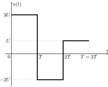
To clarify the concepts introduced in this section, it is in-teresting to consider the highly idealized system of a one-dimensional domain x ∈ (−∞, ∞) and compute the mean residence time in the control domain ω=(−∞, 0]. We as-sume that the velocity field is uniform but varies with time as in Fig. 1. Diffusion is first neglected to ease the understand-ing.
From the discussion above, the residence time is obtained as the solution ¯θof ∂ ¯θ ∂t +u(t ) ∂ ¯θ ∂x +1 = 0, x ∈ ω ¯ θ (t,0) = 0 when u(t ) >0 (10)
This equation must be integrated backwards from some “ini-tial” time T taken here as T =3T (Cf. Fig. 1). As the true “initial” conditions at that time are unknown we take
¯
θ (T , x) =0 (11)
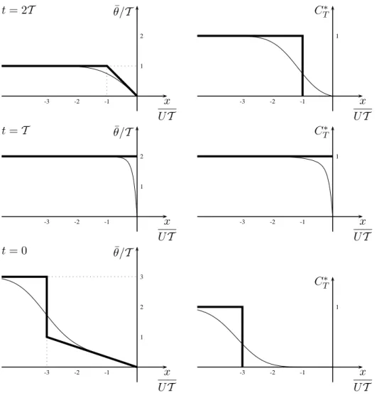
The solution of the problem Eqs. (10–11) at different times is shown in Fig. 2.
At time t =2T , the residence time varies linearly between
T at x=−U T and 0 at x=0. This is precisely the time for
a water parcel to be advected from its location at t =2T to the boundary of the control domain by the velocity field U acting between t =2T and t=3T .
The residence time for x<−U T seems to be a constant, equal to the elapsed time T of the backward simulation. This is however an artefact of the initialization of the computation at time T . The water parcels released at x<−U T at time
t =2T do not have time enough to exit the control domain; they are still in ω at t=T . Therefore the residence time of these water parcels cannot be settled since their exit time is unknown.
The resolution of the appropriate form of Eq. (8),
∂CT? ∂t +u(t ) ∂CT? ∂x =0, x ∈ ω CT?(T , x) =1, x ∈ ω CT?(t,0) = 0 when u(t ) >0 (12)
is useful to identify the part of the solution of Eq. (10) that is affected by the initialization and/or cannot be interpreted as the residence time. The solution C?
T plotted in Fig. 2
con-firms that the particles located at x<−U T at time t =2T do not leave the domain during the simulation period.
A quick look at the distribution of the control scalar at
t =T, tells us that none of the particles present in the control domain at this time can leave the control domain before t =T . Their residence time is therefore unknown. The value of ¯θis just a lower bound of the residence time.
A similar analysis can be done from the results at t=0. In this case, the residence time increases linearly from zero at
T = 3T
2T
T
0
3U
−2U
U
u(t)
t
Fig. 1. Temporal evolution of the velocity u(t ).
the origin to T at x=−3U T . The residence time cannot be computed in the leftmost part of the control domain.
Similar results are obtained if some diffusion is added to the dynamics (Fig. 2). In this case, one must solve
∂ ¯θ ∂t +u(t ) ∂ ¯θ ∂x +κ ∂2θ¯ ∂x2 =0, x ∈ ω ¯ θ (T , x) =0, x ∈ ω ¯ θ (t,0) = 0 (13) and ∂CT? ∂t +u(t ) ∂CT? ∂x +κ ∂2C¯T? ∂x2 =0, x ∈ ω CT?(T , x) =1, x ∈ ω CT?(t,0) = 0 (14)
by backward integration from t=T . Similar conclusions are obtained with, of course, smoother spatial distributions of the residence time and of the control scalar C?T. Because of diffusion, the initialization is seen to affect the results in a larger part of the control domain and/or for earlier times t . The spatial distribution of the control scalar is not strictly equal to unity in the control domain, even in its leftmost part. This shows that some water parcel can now escape the con-trol domain by diffusion within the studied time window. In such areas, ¯θprovides a lower bound for the residence time but cannot be interpreted as a valid approximation of the res-idence time unless CT? is close to zero.
4 A priori estimate of the initialization time
The computation of CT∗is useful to check the influence of the initialization a posteriori, i.e. once the simulation has been
4 E. J. M. Delhez: Transient residence and exposure times
x
UT
¯θ/T
-3 -2 -1 2 1t = 2T
x
UT
C
∗ T -3 -2 -1 1x
UT
¯θ/T
-3 -2 -1 2 1t = T
x
UT
C
∗ T -3 -2 -1 1x
UT
¯θ/T
-3 -2 -1 3 2 1t = 0
x
UT
C
∗ T -3 -2 -1 1Fig. 2. Temporal evolution of ¯θand CT∗from a backward integration of the equations for the mean residence time from t=T . Results without diffusion (thick curve) and with diffusion (thin curve, κ=U2T /4).
carried out. For practical applications, it is also desirable to have some a priori estimates of the spin-up time. A com-promise must indeed be found between the necessity to take the “initial time” T as large as possible to remove the effect of the initialization and the wish to reduce the length of the numerical simulations. Obviously, the ideal duration of the simulation depends on the residence time it-self; the larger the residence time, the larger the duration of the simulation. As a rule of thumb, one could argue that the simulation win-dow [t, T ] should be as large as twice the mean residence time for the results at time t to be significant. As the resi-dence time is not known a priori, rough estimates based on simplified models can be used to choose T .
In an advection dominated flow, the backward integration of Eq. (8) produces a front generated at the boundary of the control domain and moving into it. If Uc denotes the char-acteristic velocity of the flow and if the model is allowed to spin-up for 1t , then the space swept by the front during that
time interval can be characterized by the advective length scale Uc1t. In the meantime, horizontal diffusion smears out the front over a length scale which is some multiple α, say α=3, of the diffusion length scale
√
Kc1t where Kcis
some characteristic (explicit and implicit) horizontal diffu-sion coefficient. This spreading reduces the influence of the boundary signal in the interior of the control domain. There-fore, C∗T will be close to zero only at locations whose dis-tance to the outflow boundary of the control domain is less than
Lc=Uc1t −3√Kc1t (15)
At such locations, the residence time can be reasonably ob-tained from the solution of Eq. (6) after a spin-up time of 1t. If L denotes the horizontal dimension of the whole control domain, then the model should be allowed to spin-up for 1t such that
L ≤ Lc=Uc1t −3
√
Kc1t (16)
The estimate (15) applies reasonably well to the 1-D case discussed above if the reversal of the flow (Fig. 1) is properly taken into account. For instance, considering the initializa-tion at t=T and looking at the results at t=2T , Eq. (15) gives (taking Uc=3U and Kc=U2T /4)
Lc= −1.5U T (17)
which confirms that the residence time computed by Eq. (6) cannot be considered to be significant at any point of the control domain (Fig. 2). For the conditions prevailing for
t ∈ [0, T ] (Uc=3U and Kc=U2T /4) Eq. (15) predicts that
the initialization at time t =T would produce reasonable es-timates of the residence time at t =0 for
x >1.5U T (18)
which can be confirmed by inspection of Fig. 2.
5 Residence time vs. age theory
The two Eqs. (8) and (6) are very similar to the two equation system introduced by Delhez et al. (1999) to compute the age of tracers. In the case of a conservative tracer, these can be written as ∂C ∂t +v · ∇C = ∇ · (K · ∇C) (19) and ∂α ∂t +v · ∇α = C + ∇ · (K · ∇α) (20)
where C is the concentration of the tracer and α is the so-called age concentration. The mean age ¯a is related to C and
αby
¯ a = α
C (21)
The method discussed here for the computation of the residence time can therefore be understood as an exten-sion of the Constituent-oriented Age Theory (Delhez et al., 1999; Deleersnijder et al., 2001; Delhez and Deleersnijder, 2002). This consolidated theory is hence called “Constituent-oriented Age and Residence time Theory” (CART).
In the system (19)–(20), C measures the concentration of the tracer that, taking into account the effect of initializa-tion, contributes to the age concentration. It plays therefore a similar part as the control scalar CT∗ in the computation of the residence time. The age concentration α accumulates the contribution to the mean age of the different tracer parcels forming C. It is comparable to ¯θ.
From this similarity of the concepts, it is tempting to mod-ify the definition of the mean residence time according to
¯ θ ˜
CT∗ (22)
as only the water parcels forming ˜CT∗ are taken into account in ¯θ. This ratio would be interpreted as the mean residence time of the water parcels in ˜CT∗. However, this approach is not appropriate. The residence time is a Lagrangian property inasmuch as it can be computed for each and every water par-cel by attaching a “virtual clock” to each parpar-cel and recording its exit time from the control domain. But the path of a single virtual water parcel subjected to Fickian diffusion does not make sense in its own. The paths of different parcels form-ing a given patch are not independent from each other. This is best demonstrated by the contradiction which arises if one selects the parcels accounting for ˜CT∗(t0,x)=1−CT∗(t0,x)at some initial time t0<T and use this as initial conditions of a forward simulation; while the definition of ˜CT∗ implies that it vanishes in the control domain at time T , the forward simu-lation will produce a non zero distribution at that time. The particles accounting for ˜CT∗(t0,x)all manage to escape the control domain only because other particles immersed in the same diffusive environment remain in ω. With the Fickian model of diffusion, it is impossible to separate the fate of the particles that leave the control domain within a given time window and those that do not. The arguments leading to Eq. (22) are therefore inappropriate.
6 Residence time and exposure time
The physical interpretation of ¯θ as the mean residence time in the control domain ω depends on the boundary conditions used to solve Eqs. (3) or (6).
The residence time is usually defined as the time taken for a water parcel to leave the control domain for the first time (e.g. Bolin and Rhode, 1973; Takeoka, 1984; Zimmer-man, 1988; Monsen et al., 2003). To compute this diagnostic, called strict residence time in Delhez et al. (2004), Eq. (3) or Eq. (6) must be solved with homogenous boundary condi-tions prescribed on the boundary δω of the control domain
ω. In particular, ¯θmust vanish at the boundary of the control domain.
With such boundary conditions, water parcels leaving the domain at some time are not allowed to re-enter and
D(t, τ,x), which represents the mass in the control domain at time t +τ after a unit injection, is a decreasing function of τ . This decreasing behavior is of course expected from the interpretation of D as a cumulative distribution function. It is also required to transform the usual definition of the
6 E. J. M. Delhez: Transient residence and exposure times
x
UT
¯θ/T
-3 -2 -1 1 -2 2 1t = 2T
x
UT
C
∗ T -3 -2 -1 1 2 1x
UT
¯θ/T
-3 -2 -1 1 -2 2 1t = T
x
UT
C
∗ T -3 -2 -1 1 2 1x
UT
¯θ/T
-3 -2 -1 1 -2 3 2 1t = 0
x
UT
C
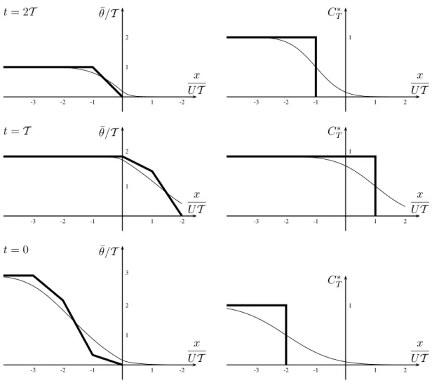
∗ T -3 -2 -1 1 2 1Fig. 3. Temporal evolution of ¯θand CT∗from a backward integration of the equations for exposure time from t=T . Results without diffusion (thick curve) and with diffusion (thin curve, κ=U2T /4).
residence time (1) into (5) along
¯ θ (t,x) = Z 1 0 τ d ˜m(t,x) = − Z ∞ 0 τ d ˜m(t,x) dt (t + τ )dτ = −hτ ˜m(t,x)(t + τ ) i∞ 0 + Z ∞ 0 ˜ m(t,x)(t + τ )dτ = Z ∞ 0 ˜ m(t,x)(t + τ )dτ = Z ∞ 0 D(t, τ,x)dτ = ¯2(t,x) (23) (assuming that ˜m(t,x)decreases to zero for large τ ).
In Delhez et al. (2004), it is proposed to solve Eqs. (3) or (6) with boundary conditions allowing the water parcels to re-enter in the control domain. In this case, the mass
˜
m(t,x)(t +τ )is no longer a decreasing function of the delay
τ. Therefore, the first equality in Eq. (23) is not valid and the solution of Eqs. (3) or (6) cannot be interpreted as the residence time any more. Still D and ¯θ have an interesting
interpretation: they can be regarded as measures of the to-tal time spent by the water parcels in the control domain. In particular, ¯θ measures the area under the curve ˜m(t,x)(t +τ )
for the whole range of values of τ (or τ in [0, T −t ] for finite range simulations). We propose therefore to call this quantity “exposure time”.
The concept of exposure time and its computation can also be demonstrated with the idealized one-dimensional system introduced above. This time, Eqs. (6) and (8) must be solved in the whole spatial domain x ∈ (−∞, ∞) without prescrib-ing auxiliary conditions at the boundary x=0 of the control domain. The results are shown in Fig. 3.
At all times and locations, the value reported for ¯θ mea-sures the total time spent by the water parcels in the control domain between the current time t and the initialization time
T. The concentration CT∗ of the control scalar can be used to identify the water parcels that are still in the control domain at t =T and those which left (and did not re-enter) the domain before that time.
3 2 1 −1 2 1
x
UT
,
¯θ
T
t/T
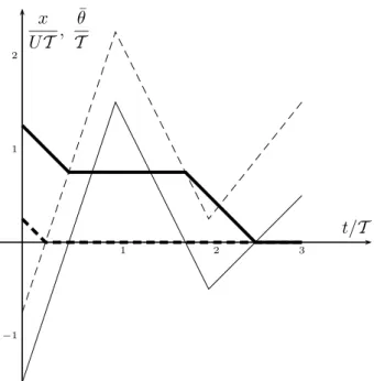
Fig. 4. Temporal evolution of the location (thin curve) and exposure time (thick curve) of particles released at x=−1.5U T (plain curve) and x=−0.75U T (dashed curve) at time t=0.
At t=2T , the spatial distributions of ¯θ and CT∗ are iden-tical to those computed in the previous section. This is of course due to the fact that the velocity is positive for
t ∈ (2T , 3T ), i.e. that all the water parcels are leaving the control domain.
Between t=2T and t =T , all the water parcels that left the domain are advected back into the control domain by the re-versing flow (Fig. 1). The value of ¯θplotted in the left panel for t =T is affected by the initialization at t=T in the range
x<U T as shown by the value of CT? in this part of the do-main. The results for x>U T are not affected by the initial-ization. The values reported for ¯θin this range can therefore be understood as the true exposure time of the water parcels, i.e. as a measure of the time spent by the water parcels in the control domain. This measure is representative inasmuch as the water parcels have left the control domain before t =T . Of course, a reversal of the flow at t >T could however push the parcels back into the control domain at later times.
Particles in x<−2U T at t=0 are still in the control do-main at t =T while those located at x>−2U T at time t =0 have all left the control domain at t =T . The latter exhibit exposure times between 0 and 2T . The stair-case distri-bution of ¯θ reflects the different paths of the parcels. As shown in Fig. 4 in the particular case of particles released at
x=−1.5U T and x=−0.75U T , some particles are present in the control domain during two distinct time intervals while others spent their time in ω in one single time interval. In both cases, the exposure time is the accumulated time spent in the control domain.
356˚ 358˚ 0˚ 2˚ 4˚ 9˚ 49˚ 0˚ 50˚ 1˚ 51˚ 2˚ 52˚ France U.K. Belgium North Sea English Channel Dover Strait A B Control region 356˚ 358˚ 0˚ 2˚ 4˚ 9˚ 49˚ 0˚ 50˚ 1˚ 51˚ 2˚ 52˚
Fig. 5. Schematic view of the general circulation in the English Channel and location of stations A and B.
Similar results are obtained when diffusion is added to the system (Fig. 3). As for the residence time, the spatial dis-tribution are smoother and the effect of the initialization is increased by diffusion. This last effect appears even worse in Fig. 3 than in Fig. 2. There is indeed no strong boundary condition at x=0 which can constrain the solution and make it converge faster.
7 Realistic application
The concepts introduced above are illustrated here with results of realistic simulations carried out with a three-dimensional hydrodynamic model of the Northwestern Eu-ropean Continental Shelf (Delhez and Martin, 1992). The model domain covers the whole shelf between 48◦N and 62◦N. The shelf break (200 m isobath) is the Western bound-ary. The model horizontal resolution is 100×100in longitude and latitude. Sigma coordinates, with 10 levels, are used in the vertical.
A schematic description of the residual circulation in this region is shown in Fig. 5. In addition to this picture, the region is known for its strong tidal signal with a characteristic tidal velocity of about 1 m/s.
For this illustration, the Eastern Basin of the English Chan-nel is taken as control domain (Fig. 5). The residence time and exposure time are computed from the results of (backward) simulations running from September 1995 to July 1993. Realistic 6 hourly wind forcing data (NCEP-reanalysis) are used to force the model.
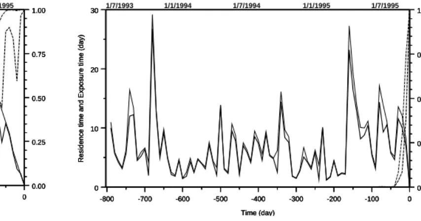
The Figs. 6 and 7 show time series of the residence time and exposure time and related control scalar concentrations at the surface at two stations A and B in the control domain (see Fig. 5 for the location of these stations). Snapshots of the spatial distribution of the residence time can be found in Delhez et al. (2004).
In both Figs. 6 and 7, the concentration of the control scalar is seen to decrease with a time scale that is of the same
8 E. J. M. Delhez: Transient residence and exposure times 0 25 50 75 100 125 150
Residence time and Exposure time (day)
-800 -700 -600 -500 -400 -300 -200 -100 0 Time (day) 0 25 50 75 100 125 150
Residence time and Exposure time (day)
-800 -700 -600 -500 -400 -300 -200 -100 0 Time (day) 0 25 50 75 100 125 150
Residence time and Exposure time (day)
-800 -700 -600 -500 -400 -300 -200 -100 0 Time (day) 0.00 0.25 0.50 0.75 1.00 0.00 0.25 0.50 0.75 1.00 0.00 0.25 0.50 0.75 1.00 1/7/1993 1/1/1994 1/7/1994 1/1/1995 1/7/1995
Fig. 6. Time series of the residence time (thick solid curve) and exposure time (light solid curve) at station A (see Fig. 5 for loca-tion). The corresponding time series for the concentration of the control scalar (right axis) are plotted with dotted lines (thick curve – residence time/light curve = exposure time).
order of magnitude as the mean residence/exposure time. The control scalar for the residence time decreases slightly more rapidly than its counterpart for the exposure time. The potential biais introduced by the initialisation procedure can be neglected after about 220 days at station A and after about 40 days at station B.
The time average values of the residence times at sta-tions A and B are, respectively, around 85 and 7 days. As expected from the definition of the two concepts, the expo-sure time is larger than the residence time at all times and locations.
The differences between the two concepts are small at sta-tion B which is located close to the downstream boundary of the control region. At station A, on the contrary, large dif-ferences are computed. The residence time at this location shows large temporal oscillations which do not appear in the time series of the exposure time. These oscillations are in-duced by episodes during which the influence at station A of the western boundary of the control domain increases (These events are poorly sampled by the 10 day model outputs and will be the subject of further investigations).
8 Conclusion
The method introduced by Delhez et al. (2004) provides a versatile tool to diagnose complex flows. In this paper, we showed how the issues of boundary conditions and initial conditions must be approached.
According to the kind of boundary conditions that are ap-plied to the numerical tracer, the method delivers the true residence time or the exposure time. Both concepts provide interesting information about the combined effects of advec-tion and diffusion and are useful in different contexts. Aware-ness about the differences of the two concepts is essential for
0 10 20 30
Residence time and Exposure time (day)
-800 -700 -600 -500 -400 -300 -200 -100 0 Time (day) 0 10 20 30
Residence time and Exposure time (day)
-800 -700 -600 -500 -400 -300 -200 -100 0 Time (day) 0 10 20 30
Residence time and Exposure time (day)
-800 -700 -600 -500 -400 -300 -200 -100 0 Time (day) 0.00 0.25 0.50 0.75 1.00 0.00 0.25 0.50 0.75 1.00 0.00 0.25 0.50 0.75 1.00 1/7/1993 1/1/1994 1/7/1994 1/1/1995 1/7/1995
Fig. 7. Time series of the residence time (thick solid curve) and exposure time (light solid curve) at station B (see Fig. 5 for loca-tion). The corresponding time series for the concentration of the control scalar (right axis) are plotted with dotted lines (thick curve – residence time/light curve = exposure time).
the correct interpretation of these diagnostics. The true res-idence time in a control domain ω measures the (average) time spent by water/tracer parcels in ω until they leave this control domain. The newly introduced exposure time mea-sures the accumulated time during which a control region is affected by a pollutant released in this region, even if the presence of the pollutant in ω is intermittent.
Both academic and realistic examples demonstrate the dif-ferent dynamics of these two diagnostics.
By resorting to the computation of a control scalar, the ef-fect of the initialization on the computed residence/exposure times can be assessed. The concentration of the control scalar must be as small as possible to avoid any bias of the results by the initialization procedure.
Acknowledgements. The author thanks E. Deleersnijder for useful
suggestions. This is MARE publication no. 75. Edited by: J. M. Huthnance
References
Bolin, B. and Rhode, H.: A note on the concepts of age distribution and residence time in natural reservoirs, Tellus, 25, 58–62, 1973. Braunschweig, F., Martins, F., Chambel, P., and Neves, R.: A methodology to estimate renewal time scales in estuaries: the Tagus Estuary case, Ocean Dynamics, 53(3), 137–145, 2003. Deleersnijder, E., Campin, J.-M., and Delhez, E. J. M.: The concept
of age in marine modelling: I. Theory and preliminary model results, J. Marine Syst., 28, 229–267, 2001.
Delhez, E. J. M. and Martin, G.: Preliminary results of 3-D baro-clinic numerical models of the mesoscale and macroscale cir-culations on the North-Western Europena Continental Shelf, J. Marine Syst., 3(4–5), 423–440, 1992.
Delhez, E. J. M., Campin, J.-M., Hirst, A. C., and Deleersnijder, E.: Toward a general theory of the age in ocean modelling, Ocean Modelling, 1, 17–27, 1999.
Delhez, E. J. M. and Deleersnijder, E.: The concept of age in marine modelling: II. Concentration distribution function in the English Channel and the North Sea, J. Marine Syst., 31, 279–297, 2002. Delhez, E. J. M., Heemink, A. W., and Deleersnijder, E.:
Resi-dence time in a semi-enclosed domain from the solution of an adjoint problem. Estuarine, Coastal and Shelf Science, 61, 691– 702, 2004.
Harley, S. J., Myers, R. A., and Field, C. A.: Hierarchical mod-els improve abundance estimates: Spawning biomass of hoki in Cook Strait, New Zealand, Ecological Applications, 14/5, 1479– 1494, 2004.
Hydes, D. J., Gowen, R. J., Holliday, N. P., Shammon, T., and Mills, D.: External and internal control of winter concentrations of nu-trients (N, P and Si) in north-west European shelf seas, Estuarine, Coastal and Shelf Science, 59/1, 151–161, 2004.
Monsen, N. E., Cloern, J. E., and Lucas, L. V.: A comment on the use of flushing time, residence time and age as transport time scales, Limnology and Oceanography, 47(5), 1545–1553, 2003.
Nixon, S. W., Ammerman, J. W., Atkinson, L. P., Berounsky, V. M., Billen, G., Boicourt, W. C., Boynton, W. R., Church, T. M., Di-toro, D. M., Elmgren, R., Garber, J. H., Giblin, A. E., Jahnke, R. A., and Owens, N. J. P.: The fate of nitrogen and phospho-rus at the land-sea margin of the North Atlantic Ocean, Bio-geochem., 35, 141–180, 1996.
Takeoka, H.: Fundamental concepts of exchange and transport time scales in a coastal sea, Continental Shelf Research, 3, 311–326, 1984.
Vollenweider, R. A.: Advances in defining critical loading levels of phosphorus in lake eutrophicatio, Mem. Ist. Ital. Idrobiol. 33, 53–83, 1976.
Wang, J. D., Luo, J., and Ault, J. S.: Flows, salinity, and some implications for larval transport in South Biscayne Bay, Florida, Bull. Marine Sci., 72/3, 695–723, 2003.
Zimmerman, J. T. F.: Estuarine residence times, in: Hydrodynamics of estuaries, edited by: Kjerfve, B., Hydrodynamics of estuaries, CRC Press, 1, 75–84, 1988.