HAL Id: hal-00924453
https://hal.archives-ouvertes.fr/hal-00924453
Submitted on 12 Jan 2021
HAL is a multi-disciplinary open access
archive for the deposit and dissemination of
sci-entific research documents, whether they are
pub-lished or not. The documents may come from
teaching and research institutions in France or
abroad, or from public or private research centers.
L’archive ouverte pluridisciplinaire HAL, est
destinée au dépôt et à la diffusion de documents
scientifiques de niveau recherche, publiés ou non,
émanant des établissements d’enseignement et de
recherche français ou étrangers, des laboratoires
publics ou privés.
atmosphere
Yung-Ching Wang, Janet G. Luhmann, François Leblanc, Xiaohua Fang,
Robert E. Johnson, Yingjuan Ma, Wing-Huen Ip, Lei Li
To cite this version:
Yung-Ching Wang, Janet G. Luhmann, François Leblanc, Xiaohua Fang, Robert E. Johnson, et al..
Modeling of the O+ pickup ion sputtering efficiency dependence on solar wind conditions for the
Martian atmosphere. Journal of Geophysical Research. Planets, Wiley-Blackwell, 2014, 119 (1),
pp.93-108. �10.1002/2013JE004413�. �hal-00924453�
RESEARCH ARTICLE
10.1002/2013JE004413
Key Points:
•When IMF strength is significantly enhanced, the sputtering effects also increase
•Sputtering escape rate of O under nominal solar wind condition is2 × 1024s−1
•Asymmetry of the sputtering effects occurs with respect to the electric fields
Correspondence to:
Yung-Ching Wang,
jinnee.ycwang@ssl.berkeley.edu
Citation:
Wang, Y.-C., J. G. Luhmann, F. Leblanc, X. Fang, R. E. Johnson, Y. Ma, W.-H. Ip, and L. Li (2014), Modeling of the O+
pickup ion sputtering efficiency dependence on solar wind condi-tions for the Martian atmosphere, J.
Geophys. Res. Planets, 119, 93–108,
doi:10.1002/2013JE004413.
Received 24 APR 2013 Accepted 18 DEC 2013
Accepted article online 20 DEC 2013 Published online 22 JAN 2014
Modeling of the O
pickup ion sputtering efficiency
dependence on solar wind conditions
for the Martian atmosphere
Yung-Ching Wang1, Janet G. Luhmann1, François Leblanc2, Xiaohua Fang3, Robert E.
Johnson4, Yingjuan Ma5, Wing-Huen Ip6, and Lei Li7
1Space Sciences Laboratory, University of California, Berkeley, California, USA,2LATMOS/IPSL-CNRS, Université Pierre et Marie Curie, France,3Laboratory for Atmospheric and Space Physics, University of Colorado Boulder, Boulder, Colorado, USA,4Department of Engineering Physics, University of Virginia, Charlottesville, Virginia, USA,5Institute of Geophysics and Planetary Physics, University of California, Los Angeles, California, USA,6Institute of Astronomy and Space Science, National Central University, Jhongli City, Taiwan,7State Key Laboratory of Space Weather, Center for Space Science and Applied Research, Chinese Academy of Sciences, Beijing, China
Abstract
Sputtering of the Martian atmosphere by O+pickup ions has been proposed as a potentiallyimportant process in the early evolution of the Martian atmosphere. In preparation for the Mars Atmosphere and Volatile Evolution (MAVEN) mission, we performed a study using a Monte Carlo model coupled to a molecular dynamic calculation to investigate the cascade sputtering effects in the region of the Martian exobase. Pickup ion fluxes based on test particle simulations in an MHD model for three different solar wind conditions are used to examine the local and global sputtering efficiencies. The resultant sputtering escape rate is 2 × 1024s−1at nominal solar wind condition and can be enhanced about 50 times
when both the interplanetary magnetic field (IMF) strength and the solar wind pressure increase. It is found that when the IMF strength becomes stronger, both the pickup ion precipitation energies and the resultant sputtering efficiencies increase. The related escape flux, hot component, and atmospheric energy deposition deduced from the MAVEN measurements may reveal clues about the prominent enhanced sputtering effects. Significant hemispheric asymmetries can be observed related to the solar wind electric fields. The shielding by the crustal fields and the recycling onto the nightside due to different magnetic field draping features can also lead to regional variations of sputtering efficiencies. The results suggest that disturbed or enhanced solar wind conditions provide the best prospects for detecting sputtering effects for MAVEN mission.
1. Introduction
The evolution of the atmosphere is a major issue in the estimation of the primitive water reservoir on Mars [Jakosky and Jones, 1997; Carr, 1999; Zuber et al., 2000; Chassefiére and Leblanc, 2004; Lammer et al., 2013]. Oxygen loss is of special interest in this problem because it can also be sequestered at and below the surface either in ice or through oxidation of rocks and minerals. Yet there is ample reason to believe that significant escape to space has occurred. The question is how much and by what process(es) [Luhmann et al., 1992; Zhang et al., 1993]. Thermal and several nonthermal escape mechanisms including photochemical reactions and the solar wind interaction were suggested to have different degrees of influences on the scavenging his-tory of the Martian atmosphere [e.g., Leblanc et al., 2002; Chassefiére and Leblanc, 2004; Chaufray et al., 2007; Lammer et al., 2013, and references therein]. While the thermal process plays a major role on the escapes of the light atoms H and He, the nonthermal mechanisms take charge of those heavier neutral escapes. Among these, pickup ion bombardment may have played an important role in earlier epochs and may be evident at present solar maximum [Luhmann and Kozyra, 1991; Luhmann et al., 1992; Johnson and Luhmann, 1998]. When planetary neutral oxygen dominant at larger altitude (approximately above the exobase at ∼ 200 km) is ionized by EUV photons, electron impacts, or charge exchange, the newly born O+will be bound by the
interplanetary magnetic fields (IMFs) and carried downstream, a process referred to as pickup. The large gyroradii of some of these ions enable them to reach high altitudes where they can escape [Luhmann, 1990; Fang et al., 2008, 2010]. However, some of them will re-impact the neutrals in the upper atmosphere, leading instead to escape of neutrals, formation of hot components in corona, and heating of the upper atmosphere
[Luhmann and Kozyra, 1991]. There are calculations of the pickup ion sputtering efficiencies for the Mars environment, obtained with both 1D [e.g., Luhmann and Kozyra, 1991; Luhmann et al., 1992; Leblanc and Johnson, 2002] and 3D [e.g., Leblanc and Johnson, 2001; Chaufray et al., 2007] simulations. The dependence of these on the solar wind conditions and on the surface crustal magnetic fields has been investigated to be important [Leblanc et al., 2002] and deserve more attention on this issue.
Based on the analysis of the Mars Express ASPERA-3 observations, Hara et al. [2011] found that the heavy ion precipitation flux will highly depend on the solar wind variations. Moreover, using Monte Carlo calcu-lations of the re-impact of O+based on the electromagnetic field background from the MHD model of the
Mars solar wind interaction [Ma et al., 2004], Li et al. [2011] suggested that nightside sputtering could occur due the magnetic draping from the dayside crustal field. Since a goal of the Mars Atmosphere and Volatile Evolution (MAVEN) mission is to understand the atmospheric escape, we initiated a study of the global and regional sputtering efficiencies in response to different solar wind conditions using realistic and sufficiently fine resolutions of previously calculated exospheric O+precipitation fluxes [Fang et al., 2013].
A Monte Carlo model of the upper atmosphere coupled to a molecular dynamic calculation for the molec-ular collisions developed by Leblanc and Johnson [2002] is applied to calculate the cascade of collisions in the region of the Martian exobase. We will introduce the basic calculation method of the atmospheric sput-tering model in section 2. In section 3, the input O+precipitation fluxes deduced from the Monte Carlo
calculations with realistic electromagnetic field distributions from a MHD model [Fang et al., 2008, 2013] are described for different solar wind conditions. The sputtering calculation results are shown in section 4, followed by a discussion of our results in section 5.
2. Atmospheric Sputtering Model
We use the atmospheric sputtering model as described in Leblanc and Johnson [2002] to calculate the cas-cade collisions by the re-impact of the pickup O+. Because when nearly reaching the exobase, the electric
field acceleration is relatively small and the incident ions will be easily neutralized by charge exchange [Luhmann and Kozyra, 1991], we trace the incident O+as neutrals as they enter the simulation domain and
assume that they are transformed to hot atoms before collision occurs. The basic 1D model is extended to 3D in order to incorporate the realistic 2D ion precipitation distributions. The initial number density and the temperature distributions of the atmosphere for both the sputtering model and the ionized neutral sources in the pickup O+calculations are chosen to be the same as each other. A uniform distribution in latitude
and longitude is used in this work. As a consequence, the regional variations in the ion precipitation and the related sputtering effects are only caused by the plasma environment and the background electromagnetic fields which affect the ionization source rates and the transport of the ions, respectively. While the input precipitation distributions of the pickup O+are adopted from previous studies of Fang et al. [2013], we will
describe the pickup ion calculations in MHD model as well as the solar wind interactions with the surface crustal fields in section 3. The atmospheric sputtering model is described as follows.
The incident particles are inserted at altitude of 300 km with downward velocities toward the surface. The global distribution of the incident particles is determined by the pickup O+precipitation distribution. A
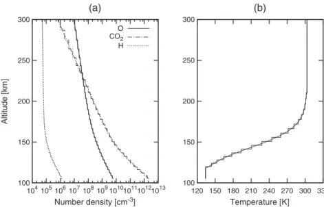
spherically uniform atmosphere is constructed from 105 to 300 km above the surface of Mars. The back-ground thermal atmosphere is built with a grid size in altitude (Δh) in logarithmic steps with the lowest one Δh0 ≈ 3.6 km and linear steps in latitude and longitude with 9◦× 9◦resolution. Three species (O,
CO2, and H) are included with altitude profiles as described in Bougher et al. [2000], Kim et al. [1998], and
Fox [2003] at solar maximum. The temperature is constraint by Mariner 6–7 observations from the model-ing calculations of Bougher et al. [2000] at solar maximum. The energetic particles includmodel-ing the incident, sputtered (collided), and backscattered ones will be traced simultaneously in both collisional domain from 105 to 300 km and collision-less domain from 300 km above the surface to 3RMfrom the center of Mars, where RM(= 3390 km) is the radius of Mars. When the particle is outside the tracing domain, it will be sup-pressed in order to accelerate the calculation. We consider those particles with energies larger than the local escape energy as escaping when they cross the upper boundary of the collisional domain (300 km above the surface). However, we still continue tracing them until their distances from the center of Mars are larger than the upper boundary of our domain (3RMfrom the center of Mars). Figure 1 shows the altitude distri-butions of the initial number densities and the temperature of the background thermal atmosphere in the collisional domain.
100 150 200 250 300 120 150 180 210 240 270 300 330 Temperature [K]
(b)
100 150 200 250 300 1041051061071081091010101110121013 Altitude [km] Number density [cm-3](a)
O CO2 HFigure 1. The initial altitude distribution of (a) the number densities of O, CO2, H and (b) the temperature of the upper atmosphere
applied in the atmospheric sputtering model. The step profiles indicate the grid size distribution along the altitude, in which the number densities and temperature are assumed to be the same.
At each time step Δt, the collisional probabilities in each cell in the collisional domain are determined [Bird, 1994]. When an energetic particle is selected to collide with the background atmosphere, a thermal particle will be created with random velocities according to the atmospheric temperature. If the energies of the particles after a collision are larger than 0.1 Eesp, where Eespis the escape energy on Mars (∼ 2 eV for O), they
will be labeled as energetic and moved with time Δt. The collisions and the transportation of particles are accomplished within one time step. Based on the particle weight and the precipitation rate, external oxygen particle are incident into the simulation domain with time step Δti, which may be larger or smaller than Δt. A quasi steady state is typically reached after ∼ 3000 s in real time. The results shown in section 4 are taken at simulated real time larger than 10,000 s. The resultant number density distribution of the sputtered hot components can be determined from a snap shot of the population of all the traced energetic particles. The setting of the energy threshold (0.1 Eesp) is chosen arbitrary by considering the calculation run time and
preserving the accuracy above ∼ 700 km at the same time [Chaufray et al., 2007]. Note that since we do not trace particles with energies lower than 0.1 Eesp, the particles with lower energies will be suppressed as a
thermal one in the collisional domain. The number density of the hot components below ∼ 700 km will then be underestimated.
The atmospheric sputtering model is adopted from Bird [1994]. The maximum number of collisions NCin the
cell C in a time step Δt is calculated with NC=
1
2NfNsFN(𝜎Tcr)maxΔt∕VC (1)
where Nfand Nsrepresent the total number of the fast (energetic) and slow (thermal) particles in cell C, FN is the weight of a simulated particle, (𝜎Tcr)maxis the maximum product of collision cross section and relative
speed before an encounter, and VCis the volume of the cell. With the introduction of a rejection criterion
determined by a random number R, an effective collision for each selected pair with various relative speed and (𝜎Tcr) can be determined [Bird, 1994]
R> 𝜎Tcr (𝜎Tcr)max
(2) This will lead to a realistic collisional probability with a mean value of every selected (𝜎Tcr). Note that only collisions between fast (> 0.1Eesp) and slow (thermal) particles are considered in the model so that the
heating of the thermosphere is not included.
When a collision occurs, the scattering is calculated using the potentials between each atom. The impact parameter of the collision is randomly chosen from 0 to b2
max, where bmaxfor O, CO2, CO, C, and H is
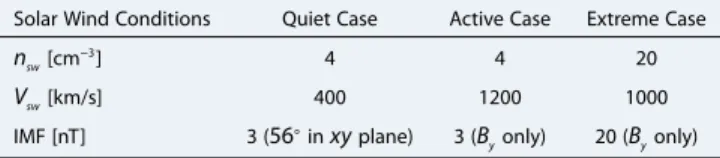
Table 1. The Solar Wind Conditions at Solar Maximum of the Simulated Cases
Solar Wind Conditions Quiet Case Active Case Extreme Case nsw[cm −3 ] 4 4 20 Vsw[km/s] 400 1200 1000 IMF [nT] 3 (56◦inxyplane) 3 (B yonly) 20 (Byonly)
Johnson et al. [2000], and Leblanc and Johnson [2002]. Within a time step, the velocities after a collision are calculated classically using semiempirical potentials to obtain the change in their velocities prior fur-ther to moving the particles. Atom-atom collision outcomes are calculated using the universal potential as described in Ziegler et al. [1985]. CO + CO collisions and collisions with energies of fast (energetic) particles of less than 10 eV are calculated by using a hard sphere approximation. Since molecular CO2is included
in the simulation, the collisions leading to dissociation are considered [Johnson and Liu, 1998]. Molecular dynamics approaches are introduced to calculate the collisions involving CO and CO2except for the CO +
CO case [Leblanc and Johnson, 2002]. The interaction potentials are described in Johnson and Liu [1998] and Johnson et al. [2000]. The integration of the motion of the colliding pair of atoms or molecules is traced until dissociation occurs or after a sufficiently long time to make sure the dissociation will not take place. Simul-taneously, the internal energies including vibration and rotation of a molecule are assumed to be preserved from one collision to the next. Although internal energy can occasionally be exchanged during long-range collisions, ignoring this should not significantly influence the resultant sputtering efficiencies [Johnson et al., 2000; Leblanc and Johnson, 2002]. The electronic energy loss is also included for collisions with the relative speed exceeding 0.5Vesp[Eckstein, 1991; Oen and Robinson, 1976], where Vespis the escape velocity on Mars
(∼ 5 km/s). The simulation results of the atmospheric sputtering model with the pickup O+precipitation
under different solar wind conditions will be discussed in section 4, including the sputtering escape flux, distributions of the hot particles, and influences of the re-impacting pick-up ions to the upper atmosphere.
3. Pickup O
+Precipitation Distribution
As an input of the atmospheric sputtering simulations, the O+precipitation distributions from previous
studies are deduced using a Monte Carlo calculation [Fang et al., 2008, 2013] with the electromagnetic field background resulting from the 3D multispecies nonideal MHD model of Ma et al. [2004] and Ma and Nagy [2007]. The solar wind conditions at solar maximum for the MHD model are summarized in Table 1, which we refer to as quiet, active, and extreme cases [Ma et al., 2004; Ma and Nagy, 2007; Fang et al., 2013] in the fol-lowing applications. The crustal magnetic field model in the MHD simulation is adopted from Arkani-Hamed [2001] with the strongest field located at noon without tilting Mars’ rotational axis. Note that only fixed crustal field location with specific IMF is studied in the present work. More case studies with different sea-sons, crustal field locations, IMF orientations, and so on are needed in order to provide us a more general concept in future.
In the test particle calculation of the pickup O+, there are 5 × 10⁹numerical O+particles in total launched
with thermal velocities and uniformly distributed in each grid from 300 km above the surface to 3RM. Each particle is weighted by the ion source rate at the production location. The ion source rate includes the effects from photoionization, electron impact, and charge exchange. The detailed ion source rates for the three mechanisms are calculated following Ma et al. [2004] and Cravens et al. [1987]. More information about the pickup O+simulations can be found in Fang et al. [2008].
The distributions of the incident energy and zenith angle with respect to the surface normal f (Ei, 𝜃i) of the re-impacting pickup O+are recorded at 300 km with a resolution of 5◦× 5◦in latitude and longitude. Due
to the limitation of computational resources in the pickup ion calculations, we preserve the incident zenith angles but assume three randomly chosen azimuth angle distributions f (𝜙i) with respect to the surface nor-mal axis in the atmospheric sputtering model. Fortunately, our tests with several specified values show that the incident azimuth angle is not the major determining parameter for the escape rates and the ejection of hot particles. Thus, only the results from the cases with the assumption of a random incident azimuth angle distribution f (𝜙i) will be discussed in section 4.
Figure 2 shows the resultant pickup O+precipitation number and energy flux distributions for the quiet case
Figure 2. The pickup O+
incident (a) number and (b) energy flux distributions at 300 km for quiet case. The (c) magnetic and (d) electric field distributions at 300 km are also shown for comparisons. The color bars of the electromagnetic fields indicate theirrcomponent, where red points outward from the surface and blue means inward directions. The square labels in Figures 2a and 2b point out the locations where the detailed pickup O+
incident energy and zenith angle spectra are shown in Figure 3.
fluxes, the enhancement in the southern hemisphere is a prominent feature in the distributions. Because the IMF is pointing from dawn to dusk at dayside, the conventional electric field (⃗E = − ⃗U × ⃗B, where ⃗Uis the bulk plasma velocity and ⃗Bis the magnetic field) generally accelerates the ions in northward directions. Conse-quently, the ions in the southern hemisphere dayside tend to re-impact the atmosphere, while those in the north mostly escape to space [c.f. Fang et al., 2008]. Although the largest re-impacting fluxes occur at the strongest crustal field regions at south, this phenomena does not imply that magnetic shielding effects do not take place. In fact, the incident energy fluxes obviously decrease at latitudes of −50◦∼ −80◦near noon.
In addition, some patchy patterns associated with the surface crustal fields can also be found. Ultimately, the precipitation fluxes and energies are controlled by the competition between the solar wind electric field acceleration and the shielding effects by the surface closed magnetic field lines. Of course, these details are specific to the particular crustal field and IMF orientations used in our study.
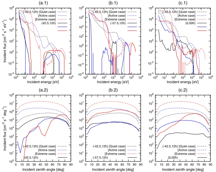
Figure 3 shows the incident energy and the zenith angle spectra at selected locations for our three sim-ulated cases. When the pickup ions travel through the background electromagnetic fields, they can be continuously accelerated by the Lorentz force. In general, if an ion is generated in the vicinity of the pre-cipitating location, its impact energy will be closer to the initial thermal one. On the other hand, if the ion is created at high altitudes from the hot corona, it will be accelerated to higher energies prior impacting to the atmosphere. Therefore, the incident energy of the particle will be as a first order dependent on dis-tance between its origin and the impact location where we assume it to be neutralized by charge exchange. Since the pickup ions with larger incident energies are mostly transported from higher altitudes, the den-sity of neutrals to be ionized is lower. Therefore, the re-impact energy spectrum will follow similar trends as the decreasing ion production rates with altitudes. As shown in Figure 3, the cutoff energy for the quiet case is at about 2 × 10⁴eV, which is consistent with the simulation results of Luhmann and Kozyra [1991] and
Chaufray et al. [2007]. If the solar wind condition becomes severe, the cutoff value can extend further toward higher energies.
We compare the incident energy and the zenith angle spectra at locations with larger inward and out-ward electric fields at latitudes of −42.5◦and 42.5◦at noon in Figure 3a and with larger magnetic shielding
effects at −57.5◦at noon in Figure 3b. Both energy spectra with large outward electric field acceleration and
crustal field shielding are depleted at medium energies. This means that only pickup ions either originating near the precipitation location or accelerated to sufficiently large energies can overcome the outward elec-tric field reflection or the magnetic shielding. Moreover, the incident zenith angle spectrum is modified by the outward electric fields, leading to larger precipitating angles with respect to the incident normal axis.
10-4 10-2 100 102 104 106 108 100 101 102 103 104 105 106 Incident flux [cm -2 s -1 eV -1 ]
Incident energy [eV]
(a.1)
(-42.5,12h) [Quiet case] [Active case] [Extreme case] (42.5,12h) 10-6 10-4 10-2 100 102 104 106 108 100 101 102 103 104 105 106Incident energy [eV]
(b.1)
(-42.5,12h) [Quiet case] [Active case] [Extreme case] (-57.5,12h) 10-4 10-2 100 102 104 106 108 100 101 102 103 104 105 106Incident energy [eV]
(c.1)
(-42.5,12h) [Quiet case] [Active case] [Extreme case] (0,00h) 100 101 102 103 104 105 106 107 108 0 10 20 30 40 50 60 70 80 90 Incident flux [cm -2 s -1 deg -1 ]Incident zenith angle [deg]
(a.2)
(-42.5,12h) [Quiet case] [Active case] [Extreme case] (42.5,12h) 100 101 102 103 104 105 106 107 108 0 10 20 30 40 50 60 70 80 90Incident zenith angle [deg]
(b.2)
(-42.5,12h) [Quiet case] [Active case] [Extreme case] (-57.5,12h) 100 101 102 103 104 105 106 107 108 0 10 20 30 40 50 60 70 80 90Incident zenith angle [deg]
(c.2)
(-42.5,12h) [Quiet case] [Active case] [Extreme case] (0,00h)
Figure 3. The pickup O+
incident (1) energy and (2) zenith angle spectra at selected locations (latitude, local time) for three cases.
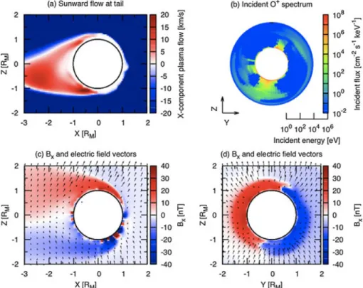
The spectra at equatorial midnight are also displayed in Figure 3c. Unlike those spectra with large depletion in the medium energy range, the energy spectrum on the nightside is more continuous. Because the surface crustal field on the dayside in the MHD model is draped by the solar wind toward the nightside and forms a taillike structure with sunward flow inside, the role of the magnetic fields there is to cause recycling of the ions rather than shielding. The sunward flow pattern in the tail in xz plane for the quiet case can be seen in Figure 4a.
In addition to the day to night and the south to north asymmetry features, there are also significant nonsym-metrical characteristics between the dawnside and duskside as shown in Figures 2a and 2b. To examine the dawn to dusk asymmetry feature in more detail, we display all the energy spectra at the terminator with the color scale in Figure 4b for the quiet case. The x component of the magnetic fields and the projected vectors of the electric fields in xz and xy planes are also shown in Figures 4c and 4d, respectively. The boundaries between ±x pointing magnetic fields due to the bending of the IMF after encountering the Mars obstacle will form a current sheet on the nightside. Due to the solar wind interactions with the magnetic anoma-lies, the orientation of the central current sheet can be modified by the alternation of the IMF direction and the respect location of the surface crustal fields, which vary with the rotation of Mars and the tilting of the rotation axis [Fang et al., 2010]. All the ions will be driven by E × B forces in the two induced magnetotail lobes and drift toward the central current sheet. The energetic ions confined within the current sheet will either escape in the pointing direction of the electric field [Fang et al., 2010] or re-impact the atmosphere due to the sunward flows in the tail [Li et al., 2011]. We can see from Figures 4b and 4d that locations with
Figure 4. (a) Thexcomponent of the plasma flow inxzplane, (b) the incident O+
energy spectrum at terminator, and (c)xcomponent of the magnetic field combined with the electric field vectors inxzand (d)yzplanes. Note that the color bar scale of the plasma flow in Figure 4a is set to be smaller than the solar wind speed in order to see the sunward flow at tail more clearly.
prominent ion re-impact fluxes with larger incident energies at the terminator are aligned with the orien-tation of the central current sheet. With the magnetic draping features simulated, higher energy fluxes will impact on the dawnside in the southern hemisphere and on the duskside in the north from tail recycling. Combined with the acceleration by the electric field, larger incident energy fluxes will occur in the south-ern hemisphere and extend dawn-ward for the simulated solar wind interaction with the surface crustal field distribution.
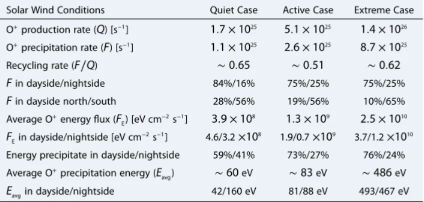
We summarize the pickup O+production rates (Q), the precipitation rates (F) and fluxes, the energy fluxes
(FE), and the average incident energy (Eavg) for the three simulated cases in Table 2. As the solar wind
con-ditions become increasingly enhanced, the plasma density may increase near the vicinity of Mars. The exospheric O can be more easily ionized by the solar wind electron impacts and solar wind proton charge exchange, leading to increasing O+production rates (Q). Although the O+precipitation rates (F) can
simul-taneously increase, this is not the case for the recycling rates (F∕Q). In fact, the global O+recycling rates
decrease as the solar wind speed becomes larger for the active case. When the solar wind condition becomes severer, we expect that the enhanced convectional electric fields will increase the asymmetry of the re-impact pickup ion flux in opposite hemispheres along the pointing of the electric fields. However, as the flow speed diverging around the obstacle becomes larger in the plasma sheath, the convectional north-ward pointing electric field does not increase equivalently to enhance the recycling rates in the southern hemisphere for the active case (see row 5 in Table 2). Since there are larger portion of pickup ions escaping from the northern hemisphere due to enhanced electric fields and larger flow speed in the plasma sheath, the global recycling rate decreases. Nevertheless, when the IMF strength also increases for the extreme case, the enhanced re-impact rate in the southern hemisphere can eliminate the effect of faster diverging flows. Therefore, the global recycling rate remains comparable as the quiet case.
We further compare the precipitation fractions on the dayside and nightside separately and find that the re-impact rates increase on the nightside for both active and extreme cases, but the total energy precipita-tion fracprecipita-tions decrease on the nightside (see row 4 and row 8 in Table 2). With faster solar wind convecprecipita-tion speeds from the nose to the tail for both active and extreme cases (see Table 1), the neutral point of the tail occurs closer to the surface, leading to smaller sunward convection rates of the ions. While the O+
Table 2. The Statistics of the Resultant Pickup O+
Precipitation Flux and Energies for Three Studied Cases
Solar Wind Conditions Quiet Case Active Case Extreme Case O+ production rate (Q) [s−1 ] 1.7 × 1025 5.1 × 1025 1.4 × 1026 O+ precipitation rate (F) [s−1 ] 1.1 × 1025 2.6 × 1025 8.7 × 1025 Recycling rate (F∕Q) ∼ 0.65 ∼ 0.51 ∼ 0.62 Fin dayside/nightside 84%/16% 75%/25% 75%/25% Fin dayside north/south 28%/56% 19%/56% 10%/65% Average O+
energy flux (FE) [eV cm −2 s−1 ] 3.9 × 10⁸ 1.3 × 10⁹ 2.5 × 10¹⁰ FEin dayside/nightside [eV cm −2 s−1 ] 4.6/3.2×108 1.9/0.7×109 3.7/1.2×1010
Energy precipitate in dayside/nightside 59%/41% 73%/27% 76%/24% Average O+precipitation energy (E
avg) ∼ 60eV ∼ 83eV ∼ 486eV Eavgin dayside/nightside 42/160 eV 81/88 eV 493/467 eV
source rates may increase due to larger densities of plasma in the tail, the nightside re-impact rates will also increase. However, as the acceleration path becomes much shorter in the tail, the recycled ion energy becomes smaller. This implies that the global and nightside recycling rates are controlled by the sunward flow in the tail, which depends on solar wind conditions, Mars’ rotation, and the seasonal tilting of the rotation axis.
Since the solar wind dynamic pressure or/and the magnetic pressure increase for active and extreme cases, the averaged incident O+energy flux (F
E) and the averaged precipitation energy (Eavg) become larger due
to the enhanced electromagnetic field strength at least in the shocked solar wind region. As both the solar wind dynamic and the magnetic pressure increase simultaneously for the extreme case, the average inci-dent energy flux (FE) can reach about 10
10eV cm−2s−1. Although this value is small compared to the solar
EUV energy flux (between 1026 and 15∐) at Mars, which is suggested to be about 5 × 10¹¹eV cm−2s−1
[Mantas and Hanson, 1985], the precipitating energy at a specific location can be large. The average incident O+energy can reach ∼ 18% (9 × 10¹⁰eV cm−2s−1) of the solar EUV in the morning sector (between dawn and
noon) on the southern hemisphere. Moreover, the pickup ion sputtering energy recycled by the sunward flow in the tail may dominate the heating of the atmosphere at the terminator and the nightside. We discuss in more details the effects of energy deposition related to the pickup O+sputtering in section 4.3.
It is important to learn which of the solar wind parameters is the major mechanism response for the vari-ation of the pickup ion precipitvari-ation fluxes and energies. We summarize the solar wind dynamic pressure and the IMF strength as well as the resultant pickup O+precipitation rates and energies, and divide them by
the values at nominal solar wind condition (quiet case) for comparisons as shown in Table 3. When the solar wind dynamic pressure increases 9 times on the dayside, the precipitation rates (F) and the average incident energies (Eavg) only increase about 2 times or less. On the other hand, if the IMF strength also increases about
6–7 times as for the extreme case, the re-impact flux and energy enhancement are about 8 times larger, and the average incident energies (Eavg) on the dayside can even reach values 12 times stronger than those
for the quiet case. As a consequence, the average incident energy flux (FE) increases more than 60 times
compared to the nominal solar wind condition. Although the solar wind dynamic pressure may increase the strength of the electromagnetic fields mainly in the shocked solar wind regions, the enhancement of the IMF strength may influence the re-impact energy flux of the pickup ion more directly rather than the dynamic pressure.
4. Sputtering Efficiencies
We apply the pickup O+precipitation flux distributions calculated from the three studied cases to the
atmo-spheric sputtering model. The resultant sputtering effects including escape, the ejected hot corona, and the influences on the upper atmosphere are discussed in the following.
4.1. Neutral Escaping Rates and Fluxes
The global sputtering yield Yifor species i is calculated as Yi=
Nesp[i]
NO+[Glancing ions included]
Table 3. The Simulated Solar Wind Parameters and the Resultant Pickup O+
Precip-itation Flux and Energies, Which Are Divided by the Values With the Nominal Solar Wind Condition (Quiet Case) for Comparisons
Solar Wind Conditions Quiet Case Active Case Extreme Case
SW dynamic pressure/[Quiet] 1 9 31.25
IMF strength/[Quiet] 1 1 6.67
(F∕Q)/[Quiet] 1 ∼ 0.8 ∼ 1.0
F/[Quiet] 1 ∼ 2.4 ∼ 7.9
FE/[Quiet] 1 ∼ 3.3 ∼ 64.1
GlobalEavg/[Quiet] 1 ∼ 1.4 ∼ 8.1
DaysideEavg/[Quiet] 1 ∼ 1.9 ∼ 11.7
where Nesp[i]is the total number of particles of species i whose energies are larger than the escape energy
when they cross the upper boundary of the collisional domain. NO+is the total number of the incident parti-cles, whose incident energy, zenith angle, and location are randomly chosen from the distributions from the test particle simulation results. If a particle is incident onto the upper atmosphere with large zenith angle, it may leave the collisional domain without encountering any neutrals due to the curvature of the exobase. These glancing ions are included in NO+. The escape yields will primarily depend on the incident energy with
smaller influences from the incident zenith angle of the particles. We examine the sputtering efficiency first before we deduce the resultant escape rates.
0 20 40 60 80 100 120 101 102 103 Yields [%]
(a)
O Quiet Active Extreme 0 0.1 0.2 0.3 0.4 0.5 0.6 101 102 103(c)
CO2 Quiet Active Extreme 0 0.005 0.01 0.015 0.02 0.025 0.03 101 102 103 Yields [%]Avg. incident energy [eV]
(d)
CO Quiet Active Extreme 0 1 2 3 4 5 6 7 8 9 10 101 102 103Avg. incident energy [eV]
(e)
C Quiet Active Extreme 0 0.1 0.2 0.3 0.4 0.5 0.6 0.7 0.8 0.9 101 102 103Avg. incident energy [eV]
(f)
Glancing ions [%] Quiet Active Extreme 0 0.05 0.1 0.15 0.2 0.25 0.3 0.35 0.4 101 102 103(b)
H Quiet Active ExtremeFigure 5. (a–e) Global sputtering yields for each species and (f ) total glancing O+
for three simulated cases with a random incident azimuth angle distribution (f (𝜙i)) assumption. The
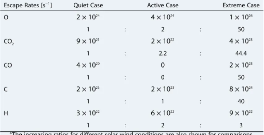
Table 4. The Global Escape Rates for Three Simulated Cases With a Random Incident Azimuth
Angle Distribution (f (𝜙i)) Assumptiona
Escape Rates [s−1
] Quiet Case Active Case Extreme Case
O 2 × 1024 4 × 1024 1 × 1026 1 : 2 : 50 CO2 9 × 10 21 2 × 10²² 4 × 10²³ 1 : 2.2 : 44.4 CO 4 × 10²⁰ 0 2 × 10²³ 1 : 0 : 50 C 2 × 10²³ 2 × 10²³ 8 × 1024 1 : 1 : 40 H 3 × 10²² 6 × 10²² 9 × 10²² 1 : 2 : 3
aThe increasing ratios for different solar wind conditions are also shown for comparisons.
Figure 5 shows the escape yields for each species versus the globally, dayside, and nightside averaged inci-dent energies for the three simulated cases. While the globally averaged inciinci-dent ion energy increases with increasing solar wind speed for the active case, the nightside averaged sputtering energy is less than 100 eV due to smaller sunward acceleration from the shorter tail behind the obstacle. Those recycled parti-cles with lower incident energies in the nightside is weighted about one quarter of the total incident rates. Although the averaged incident energy in the dayside increases, smaller escape yields in the nightside can consequently suppress the escape yields globally. Nevertheless, both the average incident energies and the sputtering yields significantly increase when the IMF strength becomes stronger (see extreme case). Except for H, the global escape yields increase about 5–7 times, although the glancing particles also slightly increase.
Table 4 shows the resultant escape rates for the three simulated cases. The increasing ratios due to solar wind variations for each species are also shown for comparisons. While the escape yields do not increase with the increasing solar wind speed, the resultant escape rates only enhance by a factor of ∼ 2 as the pickup O+precipitation rates (c.f. row 4 in Table 3) for the active case. However, as the IMF strength increases
by a factor of 6–7, the escape yields also increase accordingly. As a result, an additive increase of the sput-tered escape rates accompanied with the increasing O+precipitation rate leads to an enhancement factor
of more than 40. Therefore, we conclude that both the global incident energy of the pickup ions and resul-tant escape rate of the neutrals are determined primarily by the IMF strength rather than the speed of the solar wind.
When we compare the escape flux distributions of all five neutral species with the incident ion flux distribu-tions of the pickup O+, it is evident that the neutral escape rate is proportional to the precipitation flux of the
pickup ions, although local fluctuations can occur due to the transportation of particles. With present solar wind interactions with the surface crustal field distribution simulated in these studies, the primary region of escape neutrals is concentrated in the southern hemisphere and extended dawn-ward to the nightside as the precipitating ion flux distribution. It is interesting that the escape rates are smaller at higher latitudes in the southern hemisphere for the active case. This signature is produced by the smaller precipitation flux of the pickup ions recycled from behind the obstacle toward the terminators. While the maximum escape flux is in the order of 107− 108cm−2s−1for both quiet and active cases, the loss rates of the neutrals can reach
about 2 orders of magnitude larger with enhanced IMF strength for the extreme case. 4.2. Formation of Hot Corona
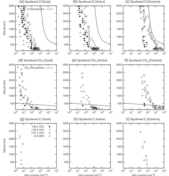
The incident energetic pickup ions not only cause escape through a cascade of collisions but produce a hot corona. Figure 6 shows the altitude profiles of the hot neutrals for O, CO2, and C for the three simulated
cases assuming a random incident azimuth angle distribution (f (𝜙i)). Four locations are chosen to see the effects from strong outward and inward electric field, shielding of the surface crustal magnetic field, and the tail recycling in the nightside at latitude of 40.5◦, −40.5◦, −57.5◦at noon, and 4.5◦at midnight, respec-tively. There is also significant south-north asymmetry in the hot corona distribution as for the pickup O+
500 1000 1500 2000 2500 3000 100 101 102 103 104 105 Altitude [km]
(a)
Sputtered O [Quiet]O Atmosphere 500 1000 1500 2000 2500 3000 100 101 102 103 104 105
(b)
Sputtered O [Active] 500 1000 1500 2000 2500 3000 100 101 102 103 104 105(c)
Sputtered O [Extreme] 500 1000 1500 2000 2500 3000 100 101 102 103 104 105 Altitude [km](d)
Sputtered CO2 [Quiet] CO2 Atmosphere 500 1000 1500 2000 2500 3000 100 101 102 103 104 105(e)
Sputtered CO2 [Active]500 1000 1500 2000 2500 3000 100 101 102 103 104 105
(f)
Sputtered CO2 [Extreme] 500 1000 1500 2000 2500 3000 100 101 102 103 104 105 Altitude [km] Hot corona [cm-3](g)
Sputtered C [Quiet] (40.5,12h) (-40.5,12h) (-67.5,12h) (4.5,00h) 500 1000 1500 2000 2500 3000 100 101 102 103 104 105 Hot corona [cm-3](h)
Sputtered C [Active] 500 1000 1500 2000 2500 3000 100 101 102 103 104 105 Hot corona [cm-3](i)
Sputtered C [Extreme]Figure 6. The altitude distribution of the sputtered hot corona at selected (latitude, local time) for species O, CO2, and C, and three simulated cases with a random incident azimuth
angle distribution (f (𝜙i)) assumption. The distribution of the nonsputtered background components for O and CO2from Ma et al. [2004] is also denoted with black lines.
produced by sputtering in the southern hemisphere. Since the hot particles can travel longer distances than the dimension of the crustal field, the hot corona densities at locations with significant surface magnetic field shielding are only slightly affected. Yet, large differences in the density at lower altitudes can still exist from one location to the other, since the major component populating the lower altitudes are the particles with lower energies. We can see that large gradient occur near altitude of 500 km between latitude −40.5◦
and −57.5◦at noon for the sputtered O corona for active case. This is caused by significant depletion of
sputtered lower energy particles at the strong magnetic field shielding location. With the formation of the sunward flow in the nightside, the number densities of the sputtered hot component may reach about the same magnitude as those in the northern hemisphere in the dayside for the active and the extreme cases. The higher re-impact flux from the tail play a role in the nightside corona formation.
100 150 200 250 300 10-3 10-2 10-1 100 101 102 103 Altitude [km]
(a)
CO Atmosphere [Quiet]100 150 200 250 300 10-3 10-2 10-1 100 101 102 103
(b)
CO Atmosphere [Active] 100 150 200 250 300 10-3 10-2 10-1 100 101 102 103(c)
CO Atmosphere [Extreme] 100 150 200 250 300 10-3 10-2 10-1 100 101 102 103 Altitude [km](d)
C Atmosphere [Quiet] (40.5,12h) (-40.5,12h) (-67.5,12h) (4.5,00h) 100 150 200 250 300 10-3 10-2 10-1 100 101 102 103(e)
C Atmosphere [Active]100 150 200 250 300 10-3 10-2 10-1 100 101 102 103
Variation of thermal component [cm-3 s-1] Variation of thermal component [cm-3 s-1]
Variation of thermal component [cm-3 s-1]
(f)
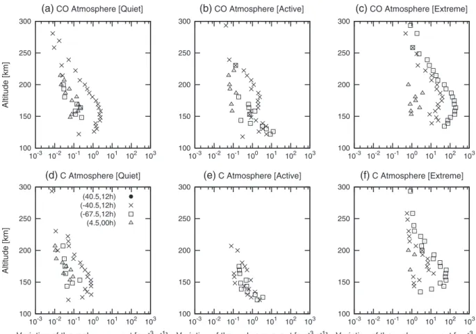
C Atmosphere [Extreme]Figure 7. The altitude distribution of the thermal (slow) component variations induced by sputtered dissociations at selected (latitude, local time) for species CO and C, and three
simulated cases with a random incident azimuth angle distribution (f (𝜙i)) assumption.
The background O and CO2atmospheres from model calculations [Bougher et al., 2000; Kim et al., 1998; Ma
et al., 2004] are also displayed for comparisons. It is seen that the sputtered component of O is negligible for nominal solar wind conditions [e.g., Chaufray et al., 2007]. In contrast, the sputtered hot component for the heavier CO2can dominate the CO2in the corona at higher altitudes. As the solar wind conditions becomes
more disturbed, the number densities of the sputter-produced hot corona increase. For the extreme case, the number density of the hot O from sputtering in the hemisphere with inward electric field may even become comparable to other sources of hot O, such as photodissociated recombination. The number densities of the heavier CO2also increase significantly to about 10
2− 103cm−3at altitudes below 3000 km.
In addition, dissociation induced by sputtering occurs and the ejected lighter C may also be detectable with densities of ∼ 102cm−3in the hemisphere with inward pointing electric fields.
4.3. Influences on the Upper Atmosphere
Besides the production of the sputtered neutrals, the incident pickup ions may also influence the structure of the upper atmospheres through cascade collisions. Because different incident azimuth angle of a particle can lead to different paths through the atmosphere, various azimuth angle distributions (f (𝜙i)) of the pickup ions will have distinct regional influences on the upper atmosphere, especially below 200 km. Therefore, the altitude profiles for the upper atmosphere shown here with the randomly distributed f (𝜙i) assumption are regarded as an average value between the neighboring regions.
In the atmospheric sputtering model, as a fast (energetic) particle is created by a collision, it is eliminated from the background thermal component in the upper atmosphere. On the contrary, if the energy of the fast (energetic) particle decreases to below 0.1 Eespafter collisions, it will be suppressed as a thermal one
and added to the background. However, the variation of the sputtered components in the upper atmo-sphere for species O, CO2, and H is relatively small in each cell compared to the initial densities. Therefore,
100 150 200 250 300 10-210-1 100 101 102 103 104 105 Altitude [km]
Ion energy loss [eV cm-3 s-1]
(a)
CO2 energy deposit [Quiet](40.5,12h) (-40.5,12h) (-67.5,12h) (4.5,00h) 100 150 200 250 300 10-210-1 100 101 102 103 104 105
Ion energy loss [eV cm-3 s-1]
(b)
CO2 energy deposit [Active]100 150 200 250 300 10-210-1 100 101 102 103 104 105
Ion energy loss [eV cm-3 s-1]
(c)
CO2 energy deposit [Extreme]Figure 8. The altitude distribution of the energy deposition from incident O+
in CO2atmosphere at selected (latitude, local time) for three simulated cases with a random incident
azimuth angle distribution (f (𝜙i)) assumption.
significant south-north asymmetry due to the electric fields occurs in the dissociated thermal components. There is almost no dissociated CO or C in the hemisphere with outward pointing electric fields. The nightside sputtering due to the tail recycling might even have larger influences on the dissociated thermal compo-nents comparing with dayside hemisphere with outward pointing electric field. The peak of the profiles is at ∼ 150–200 km with density variations of ∼ 0.1–10 cm−3s−1for the quiet and the active cases and about 1
order of magnitude larger for the extreme case.
The other interesting aspect related to the pickup ion sputtering is the incident energy deposition in the upper atmosphere through cascade collisions. Since the number density near the exobase is dominated by CO2, Figure 8 shows the energy deposition in this component. For larger incident ion energies, the particles
can penetrate deeper and deposit more energy at lower altitudes. Because the pickup ions with medium energies are easily reflected by the outward electric fields or the surface magnetic fields, the energy depo-sition profiles exhibit double-hump features at specific locations. One peak is located at ∼ 200 km, and the other is at ∼ 125 km. However, not all the incident pickup O+can penetrate deeply below nominal exobase.
Generally, only the upper atmosphere in the hemisphere with inward pointing electric fields experiences pickup ion energy deposition to altitudes below 150 km. Because near the exobase (∼ 200 km) most of the deposited energy is devoted to the formation of the hot corona, the potential heating rates cannot be estimated directly from these profiles. Therefore, we only discuss the energy deposition rates below the exobase in the present study.
For the nominal solar wind conditions (quiet case), the energy deposition rate at 125 km is less than 103eV cm−3s−1. Comparing with the solar UV energy absorption profile derived by Fox and Dalgarno
[1979, Figure 14], we can find that there is a peak absorption rate with value of ∼ 105eV cm−3s−1at 130
km. Therefore, with moderate solar wind condition, the energy deposition from the pickup ion sputter-ing can be ignored. This is consistent with the 1D modelsputter-ing result of Luhmann and Kozyra [1991]. As the solar wind dynamic pressure increases 9 times beyond the nominal value, the energy deposition at 125 km can also increase. When the IMF strength becomes stronger as well, the deposition rates can reach about 104eV cm−3s−1at lower altitudes, which is comparable with the solar UV absorption rates. Consequently, the
energy deposition to the upper atmosphere from the pickup ion sputtering may become important when the solar wind disturbed significantly.
The heating of the atmosphere by the absorption of the solar UV radiation results from the excess ener-gies carried by the photoionization or photodissociation products. Therefore, accounting for the heating efficiency the actual heating rate at 130 km is 2 × 10⁴eV cm−3s−1[Fox and Dalgarno, 1979]. Similarly, the
cascade of collisions induced by the pickup ion sputtering produces electronic, rotational, and vibrational excitations. Therefore, we should include those effects when calculating the sputtering heating rates in the future.
5. Discussions
From our case studies, we find that solar wind conditions control the pickup ion precipitation energy flux and the resulting sputtering efficiencies. Among all the variables, the IMF strength and pointing is the major factor in determining the variations in the precipitation energy flux, as well as the sputtered escape rate. For nominal solar wind conditions, the sputtered escape rate of O is about 2 × 1024s−1and the densities of the
sputtered hot neutrals below 3000 km is only about 1–102cm−3for species O and CO
2. If the IMF strength is
enhanced significantly, the global escape rate can increase more than 1 order of magnitude, and the densi-ties of the sputtered hot corona can be enhanced by 1–2 orders of magnitude over the nominal case. At the same time, effective dissociations can lead to the formation of hot neutral C with densities of approximately the same order of magnitude as those of CO2. However, we showed that the orientation of the electric field
produces asymmetries in the density profiles, resulting in less sputtered hot components in the hemisphere with outward electric fields. Since the dissociation rate also drops, there will be significant contrast between the two hemispheres in the densities of hot neutral C.
We find that if an interplanetary coronal mass ejection (ICME) encounters the Mars obstacle, the denser plasma with enhanced IMF strength in the leading pile-up region of the disturbance can increase the sput-tering efficiency considerably. Statistically, at solar maximum an ICME strikes a planetary obstacle in the ecliptic plane a couple of times per month [Jian et al., 2011]. On the other hand, when the faster solar wind takes over the slower wind, increases of the IMF strength can occur in the resulting corotating inter-action regions (CIRs). The CIRs develop mainly beyond 1 AU and may encounter Mars once per 6–7 days quasi-periodically [Hara et al., 2011]. As a consequence, we should consider the sputtering efficiencies induced by the pickup exospheric ions as dynamic perturbations even during quiet solar wind conditions. With the existence of the surface crustal field on Mars, an interesting aspect concerning the sunward flows in the tail arises [Li et al., 2011]. There has not been a detection of a taillike structure with closed field lines draping behind Mars. Yet, different solar wind conditions and the alternation of the subsolar crustal field dis-tributions can change the dimension and the orientation of the tail. This may cause difficulties in detecting a tail as the spacecraft moves along fixed orbits. Although only limited number of simulations have been carried out, they suggest that if the draping field lines do form behind Mars, additional sputtering induced by the pickup ions can take place in the nightside or extend toward the terminators led by the orientation of the central current sheet in the tail. The energetic pickup ions can be recycled back to the atmosphere along the tail structure especially for conditions of slower solar wind speed and strong crustal fields fac-ing directly into the incomfac-ing solar wind. In this situation, limb observations of the neutral emission may become more difficult to interpret with numerous variables from both solar wind and surface crustal field distributions. The magnetic shielding can also have some effects on the reflection of the pickup ions. If the solar wind electric fields point toward the south instead of the north as in our simulation cases, there may be increasing contrasts of the sputtering efficiency between the southern and the northern hemispheres. The reason is that less shielding from the crustal field with inward pointing electric field occurs in the north and stronger shielding with outward electric field in the south. Therefore, in addition to the variation of the solar wind conditions, various crustal field interactions with the IMF are an important factor controlling the sputtering efficiencies locally or globally, which should be explored in more detail in future.
We compare our quiet case results with the high solar activity simulation results of Chaufray et al. [2007], when both cases are under nominal solar wind condition with relatively hotter and denser atmosphere. From their calculation, the pickup O+production rate is about 9.4 × 1024s−1, which is only around half of
our value. While they used a 3D atmospheric distribution instead of a uniform one, the hot oxygen corona density resulting from dissociative recombination is smaller in the nightside and the terminator. Since the neutral density to be ionized decreases, the total ion production rate decreases as well. However, the pickup ion recycling rate (55%) is similar to ours. Small differences may occur due to the different grid size distribu-tion used in their hybrid model and the MHD model [Ma et al., 2004; Ma and Nagy, 2007]. In addidistribu-tion, they did not include the surface crustal fields in the hybrid simulation. The effects from the crustal field shielding and the nightside recycling from the stretched tail are not considered. As a consequence, the resultant sput-tering escape rate is also smaller with value of 7 × 10²³s−1. Their escape yield is also slightly smaller (∼ 13%)
than our O escape yield. This may due to a pure O atmosphere with three O instead of one CO2in their
molecules in our model. Yet, the pickup ion recycling rate and the sputtering escape yield are comparable for two different models.
From the above comparisons, we learn that the initial atmospheric structure is an important factor affect-ing the pickup ion production rates and the related precipitation fluxes. It is also crucial to investigate the sputtering responses corresponding to different upper atmospheric density and temperature structures. We artificially test the sputtering efficiencies using smaller O and CO2densities [see Ma et al., 2004, Figure 2] and
lower temperature (∼ 200 K isothermally at altitude> 160 km) profiles at solar minimum in the atmospheric sputtering model, when the same pickup ion precipitation distribution calculated from solar maximum atmosphere (quiet case) is used as the input. Surprisingly, we find that the sputtering results only exhibit negligible differences. The resultant escape yields are almost identical, while the differences that occur are even smaller than those when we use different incident azimuth angle (f (𝜙)) distributions for the pickup ion precipitation. The primary sputtered O and CO2hot corona is also consistent. The H escape yield increases
to 3.6% though. This is because the H density becomes about 1 order of magnitude larger [Fox, 2003] and accounts for larger portion in the upper atmosphere. While the major collisional region (exobase at ∼ 200 km) migrates toward lower altitude (∼ 150 km), the peak of the variation of the thermal dissociated com-ponents CO and C and the energy deposition rates shift downward as well. In spite of that, the peak value remains about the same. As a result, we conclude that the scale height of the density distribution and the variation of the temperature in the upper atmosphere do not significantly influence the sputtering efficien-cies when the incident pickup ion precipitation is the same. The density and the mixing ratios of different species in the exobase region is the main factor to constrain the collisional probabilities and the sputtering effects due to pickup ion precipitation.
Although the atmosphere and the exosphere structure do not influence the sputtering responses if the precipitation ions are identical, their effect on the solar wind mass loading rate, the resultant pickup ion recycling rate, and precipitation energies are significant. As the calculations from Chaufray et al. [2007] sug-gested, when the pickup ion production rate under low solar activity decreases to only about 20% of that under high solar activity, the solar wind mass loading rate becomes smaller. Since the solar wind electric field can penetrate deeper with less mass loading rate, the pickup ion recycling rate increases to 84% com-paring to 55% under high solar activity. Still, the ion precipitation rate is smaller. Similarly, we can expect the additional mass loading rate due to sputtering can decrease the pickup ion recycling rate, especially when the IMF strength is significantly enhanced. However, how the resultant precipitation rate will change is still under investigation. If the pickup ion precipitation rate does increase due to larger ion production rate, a certain saturation state can be achieved with decreasing recycling rate. Therefore, the results shown here without considering the mass loading effects from sputtering still provide a reference frame for esti-mating the sputtering efficiency varying with different solar wind conditions. The influence of sputtering on the mass loading and the energy deposition near the exobase are subjects that still need to be addressed [Johnson and Luhmann, 1998; Chaufray et al., 2007; Fang et al., 2013]. Nevertheless, while the MAVEN mis-sion will obtain pickup ion densities and speeds, atmospheric neutral and ion, and UV emismis-sion profile information, the qualitative aspects of the present results reflect what will be observed during the mission.
References
Arkani-Hamed, J. (2001), A 50-degree spherical harmonic model of the magnetic field of Mars, J. Geophys. Res., 106(E10), 23,197–23,208. Bird, G. A. (1994), Molecular Gas Dynamics and the Direct Simulation of Gas Flows, Clarendon, Oxford, England.
Bougher, S. W., S. Engel, R. G. Roble, and B. Foster (2000), Comparative terrestrial planet thermospheres: 3. Solar cycle variation of global structure and winds at solstices, J. Geophys. Res., 105(E7), 17,669–17,692.
Carr, M. H. (1999), Retention of an atmosphere on early Mars, J. Geophys. Res., 104, 21,897–21,909.
Chassefière, E., and F. Leblanc (2004), Mars atmospheric escape and evolution; interaction with the solar wind, Planet. Space Sci., 52, 1039–1058.
Chaufray, J. Y., R. Modolo, F. Leblanc, G. Chanteur, R. E. Johnson, and J. G. Luhmann (2007), Mars solar wind interaction: Formation of the Martian corona and atmospheric loss to space, J. Geophys. Res., 112, E09009, doi:10.1029/2007JE002915.
Cravens, T. E., J. U. Kozyra, A. F. Nagy, T. I. Gombosi, and M. Kurtz (1987), Electron impact ionization in the vicinity of comets, J. Geophys.
Res., 92(A7), 7341–7353.
Eckstein, W. (1991), Computer Simulation of Ion-Solid Interactions, Springer-Verlag, New York.
Fang, X., M. W. Liemohn, A. F. Nagy, Y. Ma, D. L. D. Zeeuw, J. U. Kozyra, and T. H. Zurbuchen (2008), Pickup oxygen ion velocity space and spatial distribution around Mars, J. Geophys. Res., 113, A02210, doi:10.1029/2007JA012736.
Fang, X., M. W. Liemohn, A. F. Nagy, J. G. Luhmann, and Y. Ma (2010), On the effect of the Martian crustal magnetic field on atmospheric erosion, Icarus, 206, 130–138.
Fang, X., S. W. Bougher, R. E. Johnson, J. G. Luhmann, Y. Ma, Y.-C. Wang, and M. W. Liemohn (2013), The importance of pickup oxygen ion precipitation to the Mars upper atmosphere under extreme solar wind conditions, Geophys. Res. Lett., 40, 1–6, doi:10.1002/grl.50415. Acknowledgments
We thank the reviewers for useful comments. This work was supported by NASA through the Cassini Project. The work of X. Fang was supported by NASA grant NNX11AN38G and NSF grant AST-0908472.
Fox, J. L. (2003), Effect of H2on the Martian ionosphere: Implications for atmospheric evolution, J. Geophys. Res., 108(A6), 1223,
doi:10.1029/2001JA000203.
Fox, J. L., and A. Dalgarno (1979), Ionization, luminosity, and heating of the upper atmosphere of Mars, J. Geophys. Res., 84(A12), 7315–7333.
Hara, T., K. Seki, Y. Futaana, M. Yamauchi, M. Yagi, Y. Motsumoto, M. Tokumaru, A. Fedorov, and S. Barabash (2011), Heavy-ion flux enhancement in the vicinity of the Martian ionosphere during CIR passage: Mars Express ASPERA-3 observations, J. Geophys. Res., 116, A02309, doi:10.1029/2010JA015778.
Jakosky, B. M., and J. H. Jones (1997), The histroy of Martian volatiles, Rev. Geophys., 35, 1–16.
Jian, L. K., C. T. Russell, and J. G. Luhmann (2011), Comparing solar minimum 23/24 with historical solar wind records at 1 AU, Solar Phys.,
274, 321–344.
Johnson, R. E., and M. Liu (1998), Sputtering of the atmosphere of Mars: 1. Collisional dissociation of CO2, J. Geophys. Res., 103(E2),
3639–3647.
Johnson, R. E., and J. G. Luhmann (1998), Sputter contribution to the atmospheric corona on Mars, J. Geophys. Res., 103(E2), 3649–3653. Johnson, R. E., D. Schnellenberger, and M. C. Wong (2000), The sputtering of an oxygen thermosphere by energetic O+
, J. Geophys. Res.,
105(E1), 1659–1670.
Kim, J., A. F. Nagy, J. L. Fox, and T. E. Cravens (1998), Solar cycle variability of hot oxygen atoms at Mars, J. Geophys. Res., 103(A12), 29,339–29,342.
Lammer, H. et al. (2013), Outgassing history and escape of the Martian atmosphere and water inventory, Space Sci. Rev., 174, 113–154. Leblanc, F., and R. E. Johnson (2001), Sputtering of the Martian atmosphere by solar wind pick-up ions, Planet. Space Sci., 49, 645–656. Leblanc, F., and R. E. Johnson (2002), Role of molecular species in pickup ion sputtering of Martian atmosphere, J. Geophys. Res., 107(E2),
5010, doi:10.1029/2000JE001473.
Leblanc, F., J. G. Luhmann, R. E. Johnson, and E. Chassefiere (2002), Some expected impacts of a solar energetic particle event at Mars, J.
Geophys. Res., 107(A5), 1058, doi:10.1029/2001JA900178.
Li, L., Y. Zhang, Y. Feng, X. Fang, and Y. Ma (2011), Oxygen ion precipitation in the Martian atmosphere and its relation with the crustal magnetic fields, J. Geophys. Res., 116, A08204, doi:10.1029/2010JA016249.
Luhmann, J. G. (1990), A model of the ion wake of Mars, Geophys. Res. Lett., 17(6), 869–872.
Luhmann, J. G., and J. U. Kozyra (1991), Dayside pickup oxygen ion precipitation at Venus and Mars: Spatial distributions, energy deposition and consequences, J. Geophys. Res., 96(A4), 5457–5467.
Luhmann, J. G., R. E. Johnson, and M. H. G. Zhang (1992), Evolutionary impact of sputtering of the Martian atmosphere by O+
pickup ions, Geophys. Res. Lett., 19(21), 2151–2154.
Ma, Y., and A. F. Nagy (2007), Ion escape fluxes from Mars, Geophys. Res. Lett., 34, L08201, doi:10.1029/2006GL029208.
Ma, Y., A. F. Nagy, I. V. Sokolov, and K. C. Hansen (2004), Three-dimensional, multispecies, high spatial resolution MHD studies of the solar wind interaction with Mars, J. Geophys. Res., 109, A07211, doi:10.1029/2003JA010367.
Mantas, G. P., and W. B. Hanson (1985), Evidence of solar energy deposition into the ionosphere of Mars, J. Geophys. Res., 90(A12), 12,057–12,064.
Oen, O. S., and M. T. Robinson (1976), Computer studies of the reflection of light ions from solids, Nucl. Instrum. Methods Phys. Res., 132, 647–653.
Zhang, M. H. G., J. G. Luhmann, S. W. Bougher, and A. F. Nagy (1993), The ancient Oxygen exosphere of Mars: Implications for atmosphere evolution, J. Geophys. Res., 98(E6), 10,915–10,923.
Ziegler, J. F., J. P. Biersack, and V. Littmark (1985), The Stopping and Ranges of Ions in Solids, Pergamon, New York.
Zuber, M. T., et al. (2000), Internal structure and early thermal evolution of Mars from Mars Global Survey, Topography and Gravity,